Abstract
This paper presents a comprehensive analysis of the dynamic properties of low-power current transformers (LPCTs) in the context of their application in both power systems and electromechanical systems. Momentary changes in external loads occurring in the mechanical parts of systems, affecting their correct operation, cause the appropriate monitoring and control systems, including LPCTs, to operate in transient states where dynamic errors are significant. The issues discussed in this article are therefore important from both an electrical and mechanical engineering perspective. The study focuses on the evaluation of dynamic errors using two complementary performance criteria: the mean squared error and the absolute dynamic error. An equivalent circuit model of the LPCT is formulated and employed to investigate its response under transient conditions representative of modern energy networks as well as electromechanical devices, including drives, converters, and rotating machines operating under variable loads. A key contribution of this work is the determination of the upper bounds of dynamic errors, which establish the ultimate accuracy constraints of LPCTs when subjected to rapid current variations. The obtained results provide quantitative evidence of the impact of dynamic properties on the reliability of current measurements, thereby reinforcing the importance of the proposed error evaluation framework. In this context, the study demonstrates that a rigorous assessment of dynamic errors is essential for improving the functional performance of LPCTs, particularly in applications where steady-state accuracy must be complemented by a reliable transient response.
1. Introduction
Low-power current transformers (LPCTs) [1,2] differ from conventional current transformers [3,4] in that they do not supply a secondary current of considerable power but instead generate a low-power voltage or signal proportional to the measured current [5]. This characteristic makes them particularly suitable for integration with modern measurement systems, including current transducers [6], digital platforms [7], and power quality analyzers [8]. Depending on the implementation, LPCTs may employ ferrite cores with dedicated windings integrated with electronic subsystems [9], or alternative sensing techniques such as the Hall effect [10] and other current measurement principles [11].
Today, LPCTs are a key element of modern measurement and protection systems in power grids and electromechanical systems [12]. Their advantages—high steady-state accuracy, low losses, and ease of integration with electronic systems—make them increasingly competitive with traditional current transformers [13]. However, in practice, operating conditions are rarely limited to the steady state. Transient phenomena caused by sudden load changes, switching operations, network disturbances, or the presence of higher harmonics are common [14]. In such cases, the performance of the transformer depends not only on its static accuracy but also on its behavior during rapid current variations [15]. These situations often generate dynamic errors [16,17], which can significantly distort secondary signals and impair the correct operation of protection, diagnostic, and control systems. Such current changes are inherent in practical applications, for example, in electric drives operating under variable loads or converters supplying rotating machines [18]. For these reasons, the study of dynamic properties of LPCTs is essential [19]. Mathematical analyses make it possible to quantify their accuracy and limitations under real conditions and to develop models that describe their transient behavior. The obtained results allow not only for identifying the scale of dynamic errors but also for creating methods to reduce them [17,20], which directly improves the reliability of measurement, protection, and diagnostic systems in both power generation and electromechanical environments [21,22].
The issue of dynamic errors is particularly critical during short circuits, sudden load changes, or switching processes, when rapid current variations must be correctly reflected on the secondary side [23,24]. Under these conditions, transformer cores may saturate, leading to waveform distortion and underestimation of the measured current [20]. As a result, protection devices may trip incorrectly or with a delay, compromising system reliability. In addition, transient waveforms often contain higher harmonics, which must be accurately transmitted; otherwise, errors in power quality assessment and interference with advanced measurement systems may occur [25]. Thus, dynamic errors in LPCTs can cause critical situations in which protection devices fail to react in time, exposing infrastructure to serious risks [26]. Recognizing this, contemporary standards and research emphasize the need to evaluate LPCTs not only in terms of steady-state accuracy but also during fast current changes [27]. Such studies provide the basis for developing more effective error-compensation methods aimed at improving the reliability of power and electromechanical systems. Evaluating LPCT dynamic performance requires a diverse set of test signals [28]. A sinusoidal current is used to verify steady-state accuracy [29], a ramp signal highlights dynamic errors during linear current changes [30], while a step signal examines the ability to reproduce instantaneous transients [31]. Short-circuit currents simulate overload conditions close to actual fault scenarios [32], and harmonic signals test the accuracy of representing multiple frequency components [33]. Together, these signals provide a comprehensive framework for assessing the dynamic behavior of LPCTs under realistic conditions [34]. A thorough analysis of these behaviors requires not only calculating dynamic errors for individual test signals but also determining their upper bounds relative to defined error criteria [35,36,37]. Two widely recognized approaches are the mean squared error (MSE) [38] and the absolute dynamic error (ADE) [39]. The MSE evaluates average deviations between the LPCT output and the reference by integrating squared differences, whereas the ADE indicates the maximum instantaneous error occurring during transients.
The remainder of this paper is organized as follows. Section 2 presents the equivalent circuit of the LPCT along with its transfer function model and the reference standard model used for error determination. It also provides formulas for calculating dynamic errors under five characteristic test signals and for estimating the upper bounds of the MSE and ADE. Section 3 discusses the experimental results, and Section 4 summarizes the conclusions.
The main contribution of this work lies in the development of a comprehensive procedure for determining LPCT dynamic errors together with their upper bounds. Unlike previous studies focused primarily on steady-state performance, this study systematically evaluates both the MSE and ADE under rapidly changing currents. The proposed methodology enables not only a quantitative assessment of LPCT dynamic properties across various scenarios—sinusoidal, step, ramp, short-term overload, and harmonic—but also the determination of limiting error values that define their ultimate accuracy under transient conditions. This approach allows accurate prediction of LPCT performance in real-world networks and electromechanical systems, supports the design of reliable protection and diagnostic solutions, and helps identify factors with the greatest influence on dynamic errors. Consequently, the findings improve strategies for error compensation, enhance the understanding of LPCT limitations, and contribute directly to the reliability and safety of systems in which these transformers operate as critical measurement elements.
Although numerous studies have addressed the accuracy of current transformers, most of them have focused primarily on steady-state conditions or on individual aspects of frequency response and harmonic distortion. However, there remains a lack of a unified analytical framework that quantitatively evaluates dynamic errors under transient conditions representative of real operating environments. Existing models typically do not determine the upper bounds of such errors, which are crucial for defining the ultimate accuracy limits of LPCTs. The present study addresses these gaps by introducing a comprehensive modeling and error analysis procedure that integrates an equivalent-circuit representation, transfer-function and state-space formulations, and the determination of mean squared and absolute dynamic error bounds. This combination enables a more complete characterization of LPCT performance during fast current variations and provides a methodological advancement over earlier approaches limited to steady-state analysis. This novel combination of modeling and error evaluation methods provides an original analytical contribution to the metrological study of LPCTs, offering a practical basis for assessing their performance in real transient conditions.
2. Materials and Methods
This chapter presents the mathematical foundations of modeling and analyzing the operation of low-power current transformers (LPCTs). Section 2.1 introduces the equivalent circuit of the LPCT together with the corresponding differential equations, which are subsequently transformed into the transfer function and the state-space model. Section 2.2 describes the reference model in the form of a fourth-order Butterworth band-pass filter, enabling the comparison of the LPCT output signal with the ideal reference signal. Section 2.3 focuses on the analysis of LPCT dynamic errors, including both the mean squared error (MSE) and the absolute dynamic error (ADE), as well as their estimation under worst-case conditions (UBDE). The adopted evaluation criteria and the set of test signals allow for a comprehensive analysis of the accuracy and dynamic properties of the transformer under various operating conditions.
2.1. Mathematical Model of LPCT
The behavior of a low-power current transformer (LPCT) can be rigorously characterized by means of its equivalent circuit representation. Such a model provides a formal description of the fundamental physical processes governing the device, including magnetization dynamics, core loss mechanisms, winding resistance effects, and the interaction with external measurement circuitry. The equivalent circuit serves as a convenient basis for deriving the corresponding differential equations and developing both transfer function and state-space representations. Figure 1 illustrates the equivalent circuit of the LPCT, where the measured primary current induces the secondary current through the magnetic coupling represented by the magnetizing inductance and the core-loss resistance The winding resistance, shunt resistor, load resistance, and cable capacitance represent electrical losses and the external measuring circuit. This representation enables the analysis of both steady-state and dynamic behavior of the transformer, forming the foundation for subsequent modeling and error evaluation.
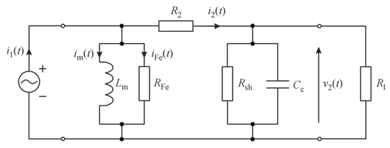
Figure 1.
Equivalent circuit of LPCT [2]. —measured current, —secondary current, —excitation inductance, —core loss resistance, —total resistance of the secondary winding and the load, —current through inductance —current through resistance —shunt sampling resistor, —capacitance of the cable, —secondary voltage, —load resistor.
From the equivalent circuit shown in Figure 1, the following differential equation can be derived [2]:
where and:
while
and
By expressing Equations (1)–(4) in the s-domain and performing the corresponding transformations, the transfer function can be obtained as follows [40]:
where is the corresponding identity matrix, and
The matrices: and denote the state matrix, input matrix and output matrix, respectively.
The corresponding state-space model is defined by the following Equations:
and
where and denote state vector and input signal, respectively.
The state and direct transmission matrices are defined as follows:
and
The input–output vectors are defined as follows:
and
The impulse response for is given by the following formula:
where
and
while
2.2. Mathematical Model of Reference
The transfer function of the four-order Butterworth band-pass filter can be obtained by transforming the corresponding transfer function of the low-pass filter, given as follows [41]:
To obtain the transfer function of the band-pass filter, the following substitution can be performed:
where and denote the angular frequency and bandwidth, respectively, while and are the lower and higher frequencies of the band-pass filter.
The symbol in Equation (17) denotes the amplification factor, while the poles are calculated using the following formula:
where denotes the filter order.
Thus, the transfer function of the band-pass filter can be expressed as follows:
where is the identity matrix, and the coefficients: and are as follows:
The corresponding state and direct transmission matrices are as follows:
and
The corresponding input–output vectors are as follows:
and
The impulse response for is given by the following formula:
where are the poles of the polynomial in the denominator on the right-hand side of the transfer function given in Equation (20).
2.3. Dynamic Error for LPCT
A low-power current transformer (LPCT) is a sensor used to measure alternating current in protection, control, and diagnostic systems, designed for minimal energy consumption. Unlike conventional electromagnetic current transformers, the LPCT utilizes a high-permeability magnetic core and a simplified winding design, making its behavior highly dependent on transient phenomena such as rapid current changes or magnetic saturation. During transients in power systems—for example, during short circuits, load transfers, or load shedding—the instantaneous current value can change many times faster than under steady-state conditions. In such situations, the transformer’s response can be delayed or distorted, leading to significant dynamic measurement errors. To date, research has focused primarily on steady-state modeling of LPCTs or frequency analysis, which provides only limited information about their dynamic properties. This creates a significant research gap in describing the behavior of these devices during rapid current changes and quantifying the resulting dynamic errors. This work aims to fill this gap by developing a comprehensive analytical approach for modeling the time-domain behavior of LPCTs and determining the upper bounds of dynamic errors. The proposed method enables a systematic assessment of the accuracy of current transformers under transient conditions and provides a basis for further development of compensation and control methods to mitigate these errors.
The response of the LPCT to an excitation in the form of the test current is given by:
where
and is the variable of integration, while denotes the total impulse response [35,36,37].
It is possible to determine the value of the dynamic error for an adopted quality criterion, based on the formula given in Equation (27). In studies of current transformers (including nonconventional LPCTs), the most commonly used criterion may be the mean squared error (MSE), given by:
where denotes the duration of the LPCT testing [35,36,37].
The error given in Equation (29) represents the squared difference between the simulated LPCT output signal and the reference signal, averaged over the period . In practice, the MSE is very convenient because it consolidates all errors over time into a single scalar value, enabling easy comparison of different transformer models or operating conditions. This error accounts for both amplitude deviations and phase shifts by evaluating the squared difference between the secondary current and the reference current throughout the entire test period, allowing assessment of the transformer’s dynamic properties, particularly its response to rapid current changes and transient overloads.
In studies of LPCTs, the absolute dynamic error (ADE) is often used alongside the MSE criterion. It is defined as follows:
In technical literature, it is a widely used and practical criterion, as it allows one to determine the maximum instantaneous deviation of the secondary signal from the reference signal, which is particularly important when analyzing the transformer’s dynamic properties. The ADE provides a simple and unambiguous measure of the peak error, regardless of the signal behavior over the considered period . It is commonly applied in electrical engineering, automation, and power and electromechanical systems, where maximum deviations are critical, for example, during transient overloads, short-circuit currents, or rapid signal changes [35,36,37]. Together, the MSE and ADE criteria complement each other by characterizing both the overall accuracy and the worst-case dynamic performance of LPCTs.
Various test signals are used to test LPCTs, depending on the test objective (static accuracy, dynamic accuracy, or overload resistance):
- Sinusoidal current—to assess static accuracy.
- Current ramp—to investigate dynamic errors during rapid current changes.
- Current step—to simulate rapid current changes and evaluate the dynamic response.
- Short-circuit current—to test resistance to transient overloads.
- Complex harmonic signal—to study the effects of harmonics and nonlinear loads.
The sinusoidal current signal is expressed by the following formula:
where denotes the frequency [Hz] of the current signal, and the parameter is determined through the following steps:
- 1.1.
- Substitute: into: given in Equation (5), where is the imaginary unit and is the angular frequency [rad/s].
- 1.2.
- Calculate: .
- 1.3.
- Find the derivative: and set it equal to 0. This gives the Equation for .
- 1.4.
- Solve the equation for .
- 1.5.
- Substitute into to find the amplification parameter .
- 1.6.
- Calculate .
The current ramp signal is expressed as follows:
where and are the initial current value, maximum current value, and ramp rise time, respectively.
The current step signal is expressed as follows:
where and are the step trigger time, initial current value, and current value after the step, respectively.
The short-circuit current signal is expressed by the following system of Equations:
where and are the rise time, peak hold time, fall time and peak current, respectively.
The complex harmonic signal is expressed as follows:
where , and are the number of harmonic components, the amplitude of the -th harmonic, the angular frequency of the -th harmonic, and the initial phase of the -th harmonic, respectively.
The upper bound on the dynamic error (UBDE) for the mean squared error criterion, constrained simultaneously in time and magnitude [42], is expressed by the following Formula:
The constrained signal is determined using the following iterative procedure:
where and are the signum function, the number of iterations assumed in advance, and the variable of integration, respectively [37,43,44]. The parameter corresponds to the magnitude constraint of the signal .
The determination of the upper bound of the dynamic error (UBDE) is carried out using an iterative fixed-point algorithm that identifies the worst-case excitation signal within predefined time and amplitude constraints. In each iteration, the algorithm updates the constrained signal to maximize the deviation between the LPCT output and the reference response, thereby converging to the input waveform that produces the maximum possible dynamic error. This approach ensures that the obtained UBDE represents the true upper limit of the error under the assumed operating conditions and provides a robust criterion for evaluating model stability and accuracy.
The upper bound on the dynamic error for the absolute dynamic error ( is expressed as follows [35,36,37]:
while the corresponding signal is determined using the following Formula:
The formulas given in Equations (36) and (38) allow estimating the worst-case scenario of dynamic error for LPCTs and determining the signals that lead to these errors, which is useful for analyzing the stability and accuracy of such devices.
3. Results and Discussion
The dynamic behavior of a low-power current transformer (LPCT) was investigated using the equivalent-circuit parameters shown in Figure 1, namely: [2]. These values are representative of typical LPCTs and served as the basis for simulating dynamic errors using Mathcad 15 software. The simulation results provide insight into the expected performance of the transformer and form the foundation for designing a comprehensive experimental setup.
This setup, intended for future verification, includes an LPCT, a function generator, an oscilloscope, a spectrum analyzer, a current amplifier, load resistors, and other necessary components, enabling practical validation of the simulation findings. The equivalent-circuit parameters used in the model (inductances, resistances, and capacitances) were selected based on typical values reported in earlier experimental studies [2] and on representative data from commercial LPCT datasheets. These values correspond to medium-range industrial sensors commonly used in power and electromechanical systems. Minor adjustments were applied to ensure numerical stability of the simulation model and consistency with the analytical assumptions presented in Section 2.
In this study, the dynamic errors were evaluated for five representative test signals: a sinusoidal current, a current ramp, a current step, a short-circuit current, and complex harmonic signals. Additionally, the upper bound on the dynamic error (UBDE) was determined according to two quality criteria: the mean squared error and the absolute dynamic error. This analysis allows for a quantitative assessment of the LPCT’s performance under varying operating conditions and establishes a reference for subsequent experimental investigations.
Let us determine the parameter . To this end, we calculate the modulus of the transfer function given in Equation (5) by substituting . Then, we have:
and
where
Equating the right-hand side of Equation (41) to zero and then solving it yields which is:
By substituting given in Equation (43) into Equation (40), we have:
By determining the parameters and based on Equation (6) and using the parameter values of the equivalent circuit, we finally obtain: For the current , the value of the parameter is equal to 52 A, according to point 1.6 included in Section 2.
The parameter represents the maximum value of the transfer function magnitude of the LPCT, which is defined as the ratio of the output voltage to the input current. This means that the parameter characterizes the maximum transfer impedance of the system, i.e., the ratio of the voltage generated at the transformer’s output to the current flowing through its primary winding, evaluated at the frequency where the amplitude response reaches its peak. Since the transfer function is expressed as , its physical dimension corresponds to resistance; therefore, the parameter is expressed in ohms . In practice, this value indicates how much voltage can be generated at the transformer’s output for a given input current under resonant conditions.
For the purposes of the conducted simulation, the following parameters were adopted: the total simulation time, corresponding to the LPCT testing interval, s, and the temporal quantization step, s.
Figure 2 shows the impulse response given in Equation (13) and obtained as the inverse Laplace transform of the transfer function given in Equation (5).
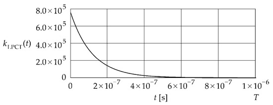
Figure 2.
Impulse response .
The impulse response exhibits an exponential decay up to approximately s, after which it asymptotically approaches a steady state. The time was assumed as the time constraint for further analysis.
Figure 3 shows the impulse response given in Equation (26) and obtained as the inverse Laplace transform of the transfer function given in Equation (20). The cut-off frequency was assumed to be equal to Hz.
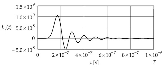
Figure 3.
Impulse response .
The impulse response exhibits a damped oscillatory behavior and attains a constant value for .
The impulse response given in Equation (28) has a shape similar to that of the impulse response due to the much smaller values of the impulse response This response serves as the basis for determining the errors: MSE, ADE and UBDE.
Figure 4 shows the sinusoidal current signal given in Equation (31) and the corresponding dynamic error calculated using Equation (27). The frequency is equal to 10 MHz.
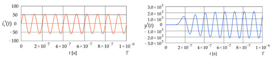
Figure 4.
Excitation current signal and corresponding error (LPCT output current calculated using the convolution integral).
The signal remains at zero until approximately s. It then gradually increases in an oscillatory manner, oscillating around values between and The value of the mean squared error given in Equation (29), is 1.71 , while the value of the absolute dynamic error given in Equation (30) is .
Figure 5 shows the current ramp signal given in Equation (32) and the corresponding dynamic error The parameters , and are assumed to be equal to 0, and , respectively
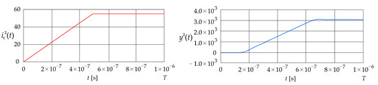
Figure 5.
Excitation current signal and corresponding error (LPCT output current calculated using the convolution integral).
The signal remains at zero until approximately s. It then increases up to about s, where it reaches approximately , and gradually settles in an oscillatory manner to around The value of the mean squared error is 5.04 , while the value of the absolute dynamic error is .
Figure 6 shows the current step signal given in Equation (33) and the corresponding dynamic error The parameters , and are assumed to be equal to 0, and , respectively.
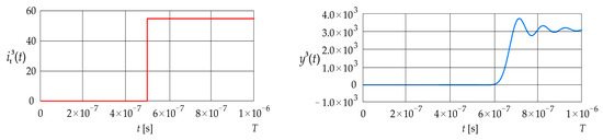
Figure 6.
Excitation current signal and corresponding error (LPCT output current calculated using the convolution integral).
The signal remains at zero until approximately s. It then increases up to about s, where it reaches approximately , and subsequently settles in an oscillatory manner to around The value of the mean squared error is 3.35 , while the value of the absolute dynamic error is .
Figure 7 shows the current step signal given in Equation (34) and the corresponding dynamic error The parameters and are assumed to be equal to , and , respectively.
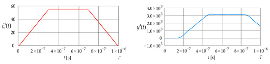
Figure 7.
Excitation current signal and corresponding error (LPCT output current calculated using the convolution integral).
The signal remains at zero until approximately s. It then increases up to about s, where it reaches approximately , and subsequently settles in an oscillatory manner until around s, reaching about . Finally, the signal decreases to approximately The value of the mean squared error is 5.75 , while the value of the absolute dynamic error is .
Figure 8 shows the complex harmonic signal given in Equation (35) and the corresponding dynamic error The parameter is equal to 4, while the current component angular frequencies and initial phases are equal to: , , and , respectively.
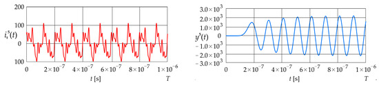
Figure 8.
Excitation current signal and corresponding error (LPCT output current calculated using the convolution integral).
The signal remains at a constant value of zero up to approximately s. It then gradually increases in an oscillatory manner, oscillating around values of and The value of the mean squared error is 1.74 , while the value of the absolute dynamic error is .
The upper bound on the dynamic error obtained for the mean squared error given in Equation (36) is 7.36 Figure 9 shows the constrained signal obtained by applying the fixed-point algorithm given in Equation (37), and the corresponding error calculated using Equation (27).
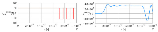
Figure 9.
Excitation current signal and error (LPCT output current calculated using the convolution integral).
The constrained signal contains five switching points, evenly distributed in time. The first switch occurs at s, and the last one at s. Up to the first switch, this signal maintains a constant value of 56 A. The signal initially rises sharply to approximately , then in the interval from s to s, it oscillates around positive values of approximately . After this, it falls to a minimum of about , then increases again, and finally decays at the end of the observed time interval. The entire waveform exhibits a transient oscillatory character with noticeable damping in its final phase.
The upper bound on the dynamic error obtained for the absolute dynamic error using Equation (38) is 6.50 Figure 10 shows the constrained signal , determined by applying Equation (39), and the corresponding error calculated using Equation (27).
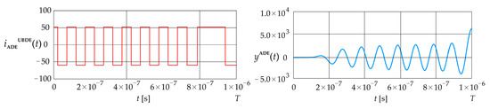
Figure 10.
Excitation current signal and error (LPCT output current calculated using the convolution integral).
The signal contains seventeen switching points that are evenly distributed over most of the interval, while the last switch occurs three times later than the preceding ones. The signal increases in an oscillatory manner and reaches its maximum value at .
Table 1 summarizes the value of the errors obtained for the signals and for both considered error criteria.

Table 1.
Value of errors obtained for the mean squared error and absolute dynamic error.
The lowest mean squared error (MSE) values were obtained for the signals and amounting to 1.71 and 1.74 , respectively, while the highest error occurs for the signal , reaching a value of 5.75 . A similar trend is observed for the absolute dynamic error (ADE), where the lowest values correspond to the signals and ( and respectively), and the highest error occurs for , amounting to . The UBDE values obtained for the signals: and represent the maximum errors for both criteria, obtained using dedicated computational procedures. This approach ensures greater accuracy in determining the maximum error values compared to the results obtained for individual signals.
The obtained results also have direct relevance for electromechanical systems, in which low-power current transformers are often integrated within control and protection loops. In such systems, rapid changes in load torque or supply voltage produce transient current variations similar to those analyzed in this study. The proposed dynamic error evaluation method makes it possible to quantify the impact of these transient phenomena on measurement accuracy, thereby improving the reliability and responsiveness of electromechanical control systems.
4. Conclusions
This study presented a comprehensive analytical framework for evaluating the dynamic errors of low-power current transformers (LPCTs) under transient operating conditions. The proposed mathematical model, based on the equivalent circuit and its transfer function and state-space representations, allows accurate assessment of dynamic performance using two complementary criteria: the mean squared error and the absolute dynamic error. The obtained results confirm that the model reliably reproduces transient electromagnetic phenomena and enables quantitative evaluation of LPCT accuracy across different excitation types. The developed approach makes it possible to determine the upper bounds of dynamic errors, which define the ultimate accuracy limits of LPCTs. These findings provide a practical foundation for improving current measurement reliability in both power and electromechanical systems. In electromechanical systems, rapid variations in load torque or supply voltage often generate transient current distortions similar to those analyzed in this study. Therefore, the proposed dynamic error evaluation framework can be directly applied to assess and improve the performance of current measurement components integrated into control and protection circuits of electric drives and other electromechanical devices. The methodology can also be used during the design and calibration of measurement transformers and extended to other sensors, such as Rogowski coils or Hall-effect devices. The proposed analytical framework extends beyond traditional impedance modeling by enabling quantitative evaluation of dynamic error limits under transient conditions, which represents a new contribution to LPCT metrological analysis.
Future research will include experimental verification of the developed model under transient operating conditions of low-power current transformers, accompanied by a parametric analysis aimed at assessing the influence of key structural and electrical parameters on dynamic errors. Moreover, the proposed methodology will be extended toward the evaluation of measurement uncertainty under dynamic conditions in accordance with ISO GUM principles. These activities will further enhance the practical relevance, reliability, and metrological consistency of the developed approach. Future research will also include validation of the developed LPCT model using hardware-in-the-loop simulation and laboratory experiments. Such verification will enable direct comparison between simulated and measured data, providing an additional confirmation of model accuracy and ensuring its reliable applicability in real operating conditions.
Author Contributions
Conceptualisation, K.T.; methodology, K.T.; software, K.T.; validation, K.T., B.R., M.S.K. and L.S.; formal analysis, K.T., B.R., M.S.K. and L.S.; investigation, K.T.; resources, K.T.; data curation, K.T. and B.R.; writing—original draft preparation, K.T.; writing—review and editing, K.T. and M.S.K.; visualisation, K.T.; supervision, K.T.; project administration, K.T.; funding acquisition, K.T. and M.S.K. All authors have read and agreed to the published version of the manuscript.
Funding
This research was conducted at the Faculty of Electrical and Computer Engineering, Cracow University of Technology, and was financially supported by the Ministry of Science and Higher Education, Republic of Poland (grant no. E-1/2025).
Data Availability Statement
The original contributions presented in this study are included in the article. Further inquiries can be directed to the corresponding author.
Conflicts of Interest
The authors declare no conflicts of interest.
References
- Mingotti, A.; Peretto, L.; Tinarelli, R. Effect of the Conductor Positioning on Low-Power Current Transformers: Inputs for the Next IEC 61869-10. Electricity 2021, 2, 1–12. [Google Scholar] [CrossRef]
- Yu, W.; Shen, H.; Hu, D.; Ni, S.; Wu, C.; Lu, X. Modeling and Transfer Characteristics Simulation Analysis of Electronic Current Transformers. J. Phys. Conf. Ser. 2024, 2903, 012012. [Google Scholar] [CrossRef]
- Burgund, D.; Nikolovski, S. Comparison of Functionality of Non-Conventional Instrument Transformers and Conventional Current Transformers in Distribution Networks. In Proceedings of the International Conference on Smart Systems and Technologies, Osijek, Croatia, 19–21 October 2022; pp. 55–60. [Google Scholar] [CrossRef]
- Kaczmarek, M.; Stano, E. Proposal for Extension of Routine Tests of the Inductive Current Transformers to Evaluation of Transformation Accuracy of Higher Harmonics. Int. J. Electr. Power Energy Syst. 2019, 113, 842–849. [Google Scholar] [CrossRef]
- Močnik, J.; Humar, J.; Žemva, A. A Non-Conventional Instrument Transformer. Measurement 2013, 46, 4114–4120. [Google Scholar] [CrossRef]
- Xiao, X.; Song, H.; Li, H. A High Accuracy AC+DC Current Transducer for Calibration. Sensors 2022, 22, 2214. [Google Scholar] [CrossRef]
- Yang, Y.; Chen, N.; Chen, H. The Digital Platform, Enterprise Digital Transformation, and Enterprise Performance of Cross-Border E-Commerce—From the Perspective of Digital Transformation and Data Elements. J. Theor. Appl. Electron. Commer. Res. 2023, 18, 777–794. [Google Scholar] [CrossRef]
- Kumar, L.A.; Indragandhi, V.; Selvamathi, R.; Vijayakumar, V.; Ravi, L.; Subramaniyaswamy, V. Design, Power Quality Analysis, and Implementation of Smart Energy Meter Using Internet of Things. Comput. Electr. Eng. 2021, 93, 107203. [Google Scholar] [CrossRef]
- Ghosh, M.K.; Gao, Y.; Dozono, H.; Muramatsu, K.; Guan, W.; Yuan, J.; Tian, C.; Chen, B. Numerical Modelling of Magnetic Characteristics of Ferrite Core Taking Account of Both Eddy Current and Displacement Current. Heliyon 2019, 5, e02229. [Google Scholar] [CrossRef]
- Lahav, D.; Schultz, M.; Amrusi, S.; Grosz, A.; Klein, L. Planar Hall Effect Magnetic Sensors with Extended Field Range. Sensors 2024, 24, 4384. [Google Scholar] [CrossRef]
- Rom, M.; van den Brom, H.E.; Houtzager, E.; van Leeuwen, R.; van der Born, D.; Rietveld, G.; Muñoz, F. Measurement System for Current Transformer Calibration from 50 Hz to 150 kHz Using a Wideband Power Analyzer. Sensors 2025, 25, 5429. [Google Scholar] [CrossRef]
- Iliev, I.; Kryukov, A.; Suslov, K.; Kodolov, N.; Kryukov, A.; Beloev, I.; Valeeva, Y. Modeling of Measuring Transducers for Relay Protection Systems of Electrical Installations. Sensors 2025, 25, 344. [Google Scholar] [CrossRef]
- Kaczmarek, M.; Szczęsny, A.; Stano, E. Operation of the Electronic Current Transformer for Transformation of Distorted Current Higher Harmonics. Energies 2022, 15, 4368. [Google Scholar] [CrossRef]
- Stano, E.; Kaczmarek, M. Analytical Method to Determine the Values of Current Error and Phase Displacement of Inductive Current Transformers during Transformation of Distorted Currents Higher Harmonics. Measurement 2022, 200, 111664. [Google Scholar] [CrossRef]
- Wang, J.; Si, D.; Tian, T.; Ren, R. Design and Experimental Study of a Current Transformer with a Stacked PCB Based on B-Dot. Sensors 2017, 17, 820. [Google Scholar] [CrossRef]
- Dichev, D.; Zhelezarov, I.; Georgiev, B.; Karadzhov, T.; Dicheva, R.; Hasanov, H. A Method for Measuring Angular Orientation with Adaptive Compensation of Dynamic Errors. Sensors 2025, 25, 4922. [Google Scholar] [CrossRef] [PubMed]
- Dichev, D.; Diakov, D.; Zhelezarov, I.; Valkov, S.; Ormanova, M.; Dicheva, R.; Kupriyanov, O. A Method for Correction of Dynamic Errors When Measuring Flat Surfaces. Sensors 2024, 24, 5154. [Google Scholar] [CrossRef]
- Pawlik, P. Single-Number Statistical Parameters in the Assessment of the Technical Condition of Machines Operating under Variable Load. Eksploat. Niezawodn. 2019, 21, 164–169. [Google Scholar] [CrossRef]
- Tomczyk, K.; Gibas, M.; Kozień, M.S. Analysis of the Dynamic Properties of the Rogowski Coil to Improve the Accuracy in Power and Electromechanical Systems. Energies 2025, 18, 4761. [Google Scholar] [CrossRef]
- Ballal, M.S.; Wath, M.G.; Suryawansh, H.M. A Novel Approach for the Error Correction of CT in the Presence of Harmonic Distortion. IEEE Trans. Instrum. Meas. 2018, 68, 4015–4027. [Google Scholar] [CrossRef]
- Hasheminejad, S. A New Protection Method for the Power Transformers Using Teager Energy Operator and a Fluctuation Identifier Index. Electr. Power Syst. Res. 2022, 213, 108776. [Google Scholar] [CrossRef]
- Odinaev, I.; Pazderin, A.; Safaraliev, M.; Kamalov, F.; Senyuk, M.; Gubin, P.Y. Detection of Current Transformer Saturation Based on Machine Learning. Mathematics 2024, 12, 389. [Google Scholar] [CrossRef]
- IEEE Std C57.13-2016; IEEE Standard Requirements for Instrument Transformers. IEEE: New York, NY, USA, 2016.
- IEC 61869-2:2012; Instrument Transformers—Part 2: Additional Requirements for Current Transformers. International Electrotechnical Commission: Geneva, Switzerland, 2012.
- Rönnberg, S.; Bollen, M. Power Quality Issues in the Electric Power System of the Future. Electr. J. 2016, 29, 49–61. [Google Scholar] [CrossRef]
- Yang, P.; Wang, T.; Yang, H.; Meng, C.; Zhang, H.; Cheng, L. The Performance of Electronic Current Transformer Fault Diagnosis Model: Using an Improved Whale Optimization Algorithm and RBF Neural Network. Electronics 2023, 12, 1066. [Google Scholar] [CrossRef]
- Krupa, M.; Gasior, M. A New Wall Current Transformer for Accurate Beam Intensity Measurements in the Large Hadron Collider. Energies 2023, 16, 7442. [Google Scholar] [CrossRef]
- Tümay, M.; Simpson, R.R.S.; El-Khatroushi, H. Dynamic Model of a Current Transformer. Int. J. Electr. Eng. Educ. 2000, 37, 247–258. [Google Scholar] [CrossRef]
- Kaczmarek, M.; Blus, K. Analytical Investigation of Primary Waveform Distortion Effect on Magnetic Flux Density in the Magnetic Core of Inductive Current Transformer and Its Transformation Accuracy. Sensors 2025, 25, 4837. [Google Scholar] [CrossRef]
- Mallette, G.; Gauthier, C.-É.; Hemmatian, M.; Denis, J.; Plante, J.-S. Design and Experimental Assessment of a Vibration Control System Driven by Low Inertia Hydrostatic Magnetorheological Actuators for Heavy Equipment. Actuators 2023, 12, 407. [Google Scholar] [CrossRef]
- Trilaksono, B.R.; Syaichu-Rohman, A.; Dronkers, C.J.; Ortega, R.; Sasongko, A. Energy Management of Fuel Cell/Battery/Supercapacitor Hybrid Power Sources Using Model Predictive Control. IEEE Trans. Ind. Inform. 2014, 10, 1992–2002. [Google Scholar] [CrossRef]
- Sun, S.; Zhou, G.; Li, Z.; Tang, X.; Zhou, Y.; Yuan, Z. Research on Measures to Limit Short-Circuit Current by Renovating the Equipment of the Power Grid. Energies 2025, 18, 2649. [Google Scholar] [CrossRef]
- Laurano, C.; Toscani, S.; Zanoni, M. A Simple Method for Compensating Harmonic Distortion in Current Transformers: Experimental Validation. Sensors 2021, 21, 2907. [Google Scholar] [CrossRef] [PubMed]
- Tomczyk, K.; Sieja, M.; Ostrowska, K.; Owczarek, D. Review of Accuracy Assessment Methods for Current Transformers: Errors, Uncertainties, and Dynamic Performance. Energies 2025, 18, 4995. [Google Scholar] [CrossRef]
- Layer, E. Modelling of Simplified Dynamical Systems; Springer: Berlin/Heidelberg, Germany, 2002; ISBN 978-3-540-43762-8. [Google Scholar]
- Tomczyk, K. Special Signals in the Calibration of Systems for Measuring Dynamic Quantities. Measurement 2014, 49, 148–152. [Google Scholar] [CrossRef]
- Tomczyk, K. Monte Carlo based procedure for determining the maximum energy at the output of accelerometers. Energies 2020, 13, 1552. [Google Scholar] [CrossRef]
- Hodson, T.; Over, T.M.; Foks, S. Mean Squared Error, Deconstructed. J. Adv. Model. Earth Syst. 2021, 13, e2021MS002681. [Google Scholar] [CrossRef]
- Frías-Paredes, L.; Mallor, F.; Gastón-Romeo, M.; León, T. Dynamic Mean Absolute Error as New Measure for Assessing Forecasting Errors. Energy Convers. Manag. 2018, 162, 176–188. [Google Scholar] [CrossRef]
- Solovev, D.B.; Gorkavyy, M.A. Current Transformers: Transfer Functions, Frequency Response, and Static Measurement Error. In Proceedings of the 2019 International Science and Technology Conference EastConf, Vladivostok, Russia, 20–21 September 2019; IEEE: New York, NY, USA, 2019; pp. 1–6. [Google Scholar]
- Sadiq, A.A.; Othman, N.B.; Abdul Jamil, M.M.; Youseffi, M.; Denyer, M.; Wan Zakaria, W.N.; Md Tomari, M.R. Fourth-Order Butterworth Active Bandpass Filter Design for Single-Sided Magnetic Particle Imaging Scanner. J. Telecommun. Electron. Comput. Eng. 2025, 10, 1–17. [Google Scholar]
- Rutland, N.K. The principle of matching: Practical conditions for systems with inputs restricted in magnitude and rate of change. IEEE Trans. Autom. Control. 1994, 39, 550–553. [Google Scholar] [CrossRef]
- Elia, M.; Taricco, G.; Viterbo, E. Optimal energy transfer in band-limited communication channels. IEEE Trans. Inf. Theory 1999, 45, 2020–2029. [Google Scholar] [CrossRef][Green Version]
- Long, G.; Nelakanti, G. Iteration methods for Fredholm integral equations of the second kind. Comput. Math. Appl. 2006, 53, 886–894. [Google Scholar] [CrossRef]


Disclaimer/Publisher’s Note: The statements, opinions and data contained in all publications are solely those of the individual author(s) and contributor(s) and not of MDPI and/or the editor(s). MDPI and/or the editor(s) disclaim responsibility for any injury to people or property resulting from any ideas, methods, instructions or products referred to in the content. |
© 2025 by the authors. Licensee MDPI, Basel, Switzerland. This article is an open access article distributed under the terms and conditions of the Creative Commons Attribution (CC BY) license (https://creativecommons.org/licenses/by/4.0/).