Development and Verification of a Transient Analysis Tool for Solar Power Tower System with sCO₂ Brayton Cycle

Abstract

Supercritical carbon dioxide (sCO₂) Brayton cycle is a promising technology for concentrating solar power systems. However, existing studies predominantly rely on steady-state or quasi-steady-state assumptions, thereby neglecting transient characteristics of fluid flow and heat transfer. This study develops a transient analysis program for solar power tower systems integrated with sCO₂ Brayton cycles using the finite difference method. The program comprises two interactive modules—a molten salt loop and a Brayton cycle module—coupled through an intermediate heat exchanger. For the Brayton cycle module, a fluid network model enabling a unified framework for the simultaneous solution of all governing equations is adopted. The SIMPLE algorithm and Gauss–Seidel iteration method are employed to solve the conservation equations. Following validation of key components and system performance, dynamic simulations under load and solar irradiance step disturbances are conducted. The results demonstrate that the program accurately captures transient behaviors and supports control strategy design and safety analysis for solar power tower systems with arbitrary sCO₂ Brayton cycle layouts.

1. Introduction

Solar energy is a kind of promising energy [1] and is important for sustainable energy development [2]. Its large-scale utilizations mainly include solar photovoltaic [3] and solar thermal utilizations [4]. Concentrating solar power (CSP) is increasingly acknowledged as an effective technology for the future electricity market [5]. In recent years, it has drawn lots of attention due to its compact configuration, high thermal efficiency, and low compressor consumption power [6]. The supercritical carbon dioxide (sCO₂) Brayton cycle power conversion technology is deemed the most promising technical solution for future CSP systems [7]. To boost its development, researchers have conducted extensive studies to clarify the characteristics of the overall system [8]. Based on research objectives and simulation models’ assumptions, the thermodynamic analysis of an sCO₂-CSP integrated power generation system can be categorized into three levels: design condition analysis, off-design condition analysis, and transient analysis.

The objective of design condition analysis is to determine the cycle’s thermodynamic parameters and the key performance parameters of major components under specified boundary conditions. This analysis serves as the foundation for thermodynamic research and provides essential input parameters for subsequent off-design condition and dynamic analyses. Li et al. [9] developed a comprehensive one-dimensional component model for key components in sCO₂ Brayton cycles and applied this model to the multi-objective optimization of an sCO₂ Brayton cycle with a net power of 50 MW. The Meryame research group [10] studied an integrated CSP system in arid regions, focusing on evaluating the thermodynamic performance of simple and recompression sCO₂ Brayton cycles across different power scales. Zhai et al. [11], using operating parameters from a CSP system as boundary conditions, employed intelligent algorithms to optimize the flow distribution and design parameters of multiple cycle configurations for maximum specific power output and enhanced heat exchanger network performance. However, these studies mainly focus on the optimization of Brayton cycle parameters, and the impact of CSP components’ behavior on the overall system performance was ignored. Li et al. [12] introduced a novel solar receiver, developed a corresponding mathematical model, and optimized system performance using orthogonal experiments and a genetic algorithm. This novel solar receiver showed higher thermal efficiency under high-temperature operating conditions. Based on the research of Tao et al. [13], an innovative configuration for a printed circuit heat exchanger (PCHE) in the sCO₂ Brayton cycle was proposed, integrating straight and airfoil-shaped grooves to mitigate high stress concentration at the fin tips.

The objective of off-design condition analysis is to clarify the performance of a given system under off-design conditions. It is usually conducted based on the results from the design condition analysis. Li et al. [9] conducted an off-design analysis using a one-dimensional sCO₂ Brayton cycle model. They demonstrated that even with a main compressor inlet temperature variation of up to 5 K, cycle efficiency fluctuations could be maintained within 1.0% through an inventory control strategy. Furthermore, by combining inventory control with main compressor inlet pressure control, the system’s net power could remain stable under ambient temperature fluctuation conditions. Similarly, Meryame et al. [10] reported in their off-design analysis that an increase in compressor inlet temperature reduced the thermal efficiency and power output of both simple and recompression Brayton cycles. It also concluded that the simple configuration is more suitable for arid regions than the recompression configuration, owing to its comparable thermal efficiency at an inlet temperature of 55 °C and its inherently simpler layout. Battisti et al. [14] developed a computational model using the Engineering Equation Solver (EES) and the System Advisor Model (SAM) to evaluate two solar-powered sCO₂ recompression Brayton cycle systems in northern Chile. The annual simulation results revealed that exergy destruction in the gas cooler increased at high ambient temperatures, similar to the trend observed in the turbine during off-design operations. Lu et al. [15] developed a MATLAB-based model to analyze the off-design performance of sCO₂ Brayton cycles for solar power generation. The off-design performance over both annual and daily timescales for simple regenerative and recompression configurations is investigated based on this model. It was found that under off-design conditions, the recompression configuration with a specific bypass fraction exhibited better performance.

A brief, off-design condition analysis enables the evaluation of thermal efficiency characteristics for different configurations under various load and ambient scenarios, as well as the development of effective load control strategies. However, it should be noted that the off-design models reviewed were predominantly developed based on steady-state or quasi-steady-state assumptions. This implies that these models can only evaluate steady-state performance after boundary conditions (e.g., load, DNI, ambient temperature) change, while neglecting the transient process of system transition between states. The dynamic response of a system during transition phases, which occur when boundary conditions change and the system shifts from one operational state to another, is critical for control system design, control strategy optimization, and system safety performance evaluation. The primary objective of transient analysis is to conduct research on this specific topic by utilizing transient models. Currently, research on transient analysis for tower solar thermal power generation systems is still relatively limited, particularly concerning transient behavior in systems integrated with sCO₂ Brayton cycles. Some recent achievements in the transient analysis of solar Brayton cycles are presented in Table 1.

Table 1. Partial results of transient models for CSP and sCO₂ Brayton cycles.

Sources	Research Contents & Key Findings	Limitations & Shortcomings
Chen et al. [16]	Developed a transient model for a solar tower sCO2 cycle. Used a 1-D dynamic heat exchanger model. Finding: Cloud disturbances (DNI variation) caused a 114.65 K temperature fluctuation at the PCHE outlet, creating high thermal stress.	Model was simplified and lacked a thermal energy storage (TES) system.
Yuet al. [17]	Built a lumped parameter model for a 200.0 kWe plant on TRNSYS. Finding: Outlet temperatures were highly sensitive to DNI. Receiver efficiency remained stable at ~0.7.	Model is not generalizable; a new model is needed for different plants.
Delsoto et al. [18]	Created a finite volume model with inventory control for a 10.0 MW plant. Accurately captured power output dynamics and studied TES/collector field size impact.	Ignored pressure effects and did not use the momentum equation.
Wang et al. [19]	Established a lumped parameter model for a solar-coal hybrid plant to analyze dynamics and achieve high solar efficiency.	Also ignored the influence of pressure on the system’s response.

Chen et al. [16] developed a transient model for a tower-type solar indirect heating sCO₂ Brayton cycle. The model was solved using the gPROMS solver, which employed either the modified Euler method or a fully implicit Runge–Kutta method. The heat exchanger was modeled as a one-dimensional dynamic model. The results showed that during cloud-disturbed operation (DNI variation: 700.0–780.0 W/m²), the cold-side sCO₂ outlet temperature of the PCHE fluctuated by 114.65 K in a short time, posing significant thermal stress on the component. However, an energy storage system was not considered in this model. Yu et al. [17] developed a transient model based on the lumped parameter method for a 200 kW sCO₂ solar thermal power station. The model was implemented on the TRNSYS platform to investigate the system dynamic responses under variations in key parameters like DNI. The results showed a significant and highly sensitive positive correlation between sCO₂ outlet temperature and DNI. The particle receiver efficiency remained approximately stable at 0.7 across varying weather conditions. A key limitation was the model’s specificity to this particular plant design, limiting its transferability to other configurations without significant modification. Delsoto et al. [18] established a transient model with an inventory control method for a 10 MW solar power station using the finite volume method. This model accurately reflected the power plant’s power output dynamics. The study also investigated the impact of thermal energy storage system size and solar collector field size on system dynamics. A drawback was that pressure effects were ignored during mathematical modeling, and the momentum equation was not considered. Wang et al. [19] developed a transient model of a solar-coal hybrid power station using the lumped parameter method. The model was capable of analyzing the power station’s dynamics. However, it overlooked the influence of pressure on the system’s dynamic response.

According to the review above, it can be found that some limitations occur for the transient analysis of tower-type solar thermal power generation systems. Most existing models are built for specific power stations. Although these models can effectively evaluate the system’s transient response characteristics, they have limitations in the scalability of Brayton cycle architectures [20]. This paper aims to develop a transient analysis tool for studying the control strategy, dynamic characteristics, and safety performance of an integrated SPT system coupled with various sCO₂ Brayton cycles, as illustrated in Figure 1. The advances of the developed analysis code relies on two aspects: (1) transient governing models for fluid mass, momentum and energy conservation functions, as well as for metal heat conduction are established to predict the system’s transient response under various scenarios; (2) the development of a generic fluid network model for the Brayton cycle side, enabling predictive capability for various configurations (e.g., recompression cycle, intercooling cycle, etc.) without requiring modifications to the cycle solution strategy.

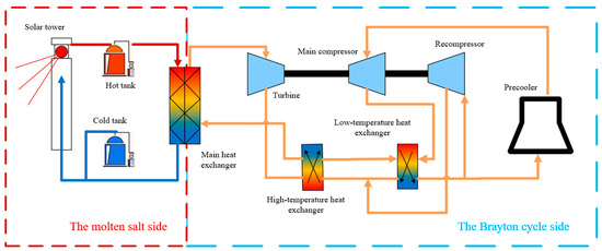
Figure 1. Schematic diagram of a tower-type solar power generation system. The red line segments with arrows represent the hot molten salt fluid, the dark blue represents the cold molten salt fluid, and the orange represents the sCO₂ fluid.

The organization of this paper is as follows. Section 1 reviews recent studies on thermodynamic analysis methods for SPT systems coupled with sCO₂ Brayton Cycles. Section 2 describes the methods for model development, including the molten salt-side models, the sCO₂ Brayton cycle-side models, and the molten salt cycle/sCO₂ Brayton cycle coupling approach. Section 3 conducts the model validation at both the component and system levels, and demonstrates the application and predictive capability of the developed tool via a load-following scenario of an integrated system. Section 4 further provides a discussion on the capabilities and limitations of the developed tool. Finally, Section 5 summarizes the main conclusions and drawbacks of the developed transient analysis tool.

2. Methods

As shown in Figure 1, the entire system is divided into two modules: the molten salt side and the Brayton cycle side. The molten salt side and the Brayton cycle side are coupled through an intermediate heat exchanger. In this section, separate component models and a coupling method for the two modules are developed. In Section 2.1, the physical property model of fluids is described. The detailed descriptions of models for the molten salt side and Brayton cycle side are presented in Section 2.2 and Section 2.3, respectively. The coupling method of the molten salt side and Brayton cycle side can be found in Section 2.4.

2.1. Physical Property Model

In the SPT system, molten salt (60% NaNO₃-40% KNO₃) is chosen as the heat transfer fluid and thermal energy storage medium. The thermophysical properties of the molten salt are obtained by fitting the data in ref. [21]. The fitting expressions are shown in Table 2. All physical parameters are functions of temperature T, and its operating temperature range is 270.0–600.0 °C. The working medium on the Brayton side is supercritical carbon dioxide.

Table 2. Thermal physical properties of molten salts.

Item	Value
Density (kg/m3)	$\rho =2090-0.636T$;	(1)
specific heat capacity (J/kg⋅K)	$C_p=1443+0.172T$;	(2)
Thermal conductivity (W/m⋅K)	$\lambda =0.443+1.9\times {10}^{-4}T$;	(3)
Dynamic viscosity (MPa/s)	$\mu =22.714-0.12T+2.281\times {10}^{-4}{T}^2-1.474\times {10}^{-7}{T}^3$.	(4)

The physical properties of CO₂ are the foundation for simulating the sCO₂ Brayton cycle system. The CO₂ physical property call model developed in this paper is based on the NIST physical property library. A set of thermophysical property correlations for supercritical carbon dioxide is developed based on the NIST reference property database. The properties include specific heat capacity, thermal conductivity, density, and temperature, among others, all expressed as functions of state variables. The applicable range of the sCO₂ physical property package is as follows: pressure from 0.1 to 25 MPa and specific enthalpy from 200 to 1600 kJ/kg.

2.2. Modeling Method for Molten Salt Side

As shown in Figure 1, the molten salt system module mainly has four components, including the solar collector, high-temperature molten salt storage tank, low-temperature molten salt storage tank, and intermediate heat exchanger for heat exchange between molten salt and sCO₂. To simplify the calculation, the working fluid is assumed to be a single-phase flow, and the frictional losses and heat losses in pipelines are neglected in the molten salt loop. In addition, the molten salt loop is solved using a sequential modular approach, wherein the governing equations for each component are solved in the predetermined order. And, the first-order upwind difference method is used for discretization. The detailed governing models of the component for molten salt side are described below.

2.2.1. Solar Collector Model

The traditional solar collector model has a cylindrical structure made up of 24 heat-absorbing light panels. These panels are arranged in two parallel columns, and to ensure uniform heating of the internal fluid, a cross-flow pattern is used. Each group of 12 heat-absorbing light panels is connected in series, with the specific arrangement shown in Figure 2. In the solar power generation system, molten salt has no phase change, and its physical properties are only influenced by temperature. Also, the external heat-absorbing light panel structures of the tower solar collector are exactly the same. Thus, it can be equivalently modeled as a sufficiently long heat-absorbing tube, which is conducive to subsequent model simulation and solution. When modeling this equivalent collector, given that the solar radiation received by the collector pipes differs at various positions [22], the heat-absorbing tube is divided into n heat-absorbing segments of length dx along the fluid flow direction. Meanwhile, it is assumed that the heat absorbed by each unit is evenly distributed.

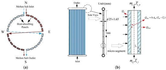
Figure 2. Collector model structure: (a) and single-tube micro-segment; (b) modeling [22].

The thermal power required by the solar collector is obtained from the heliostat field and input into the collector as a heat source term [23]:

$$P_{\mathrm{h}}=N_{\mathrm{h}}{S}_{\mathrm{h}}DNI{\eta }_{\mathrm{op}},$$

(5)

where N_h is the number of heliostats in the heliostat field. S_h is the area of a single heliostat. DNI is the direct radiation power received per unit area perpendicular to the solar incident direction. η_op is the concentration efficiency of the heliostat field.

The fluid conservation equations in the collector pipeline are shown in Equations (6) to (8). The energy conservation equation is shown in Equation (6):

$$M_{\mathrm{rec}}{C}_{\mathrm{rec}}{\displaystyle \frac{dT}{dt}}=P_{\mathrm{h}}+m_{\mathrm{rec},\mathrm{in}}{h}_{\mathrm{rec},\mathrm{in}}-m_{\mathrm{rec},\mathrm{out}}{h}_{\mathrm{rec},\mathrm{out}}.$$

(6)

The mass conservation equation is shown in Equation (7):

$${\displaystyle \frac{d{M}_{\mathrm{rec}}}{dt}}={\displaystyle \sum m_{\mathrm{rec},\mathrm{in}}}-{\displaystyle \sum m_{\mathrm{rec},\mathrm{out}}}.$$

(7)

The momentum conservation equation is shown in Equation (8):

$$\Delta P_{\mathrm{rec}}-\lambda {\displaystyle \frac{L}{d}}({\displaystyle \frac{{\rho }_{\mathrm{rec}}{u_{\mathrm{rec}}}^2}{2}})-{\xi }_{\mathrm{rec}}({\displaystyle \frac{{\rho }_{\mathrm{rec}}{u_{\mathrm{rec}}}^2}{2}})-{\rho }_{\mathrm{rec}}{g}_{\mathrm{rec}}H={\displaystyle \frac{L}{A}}{\displaystyle \frac{\partial m_{\mathrm{rec}}}{\partial \mathrm{t}}},$$

(8)

where m_rec is the collector flow rate. M_rec is the collector mass. ΔP_rec is the pressure drop of the collector. λ is the friction loss coefficient along the way. ρ_rec is the density. u_rec is the flow velocity. L is the length of the flow channel. d is the equivalent diameter. ξ_rec is the local loss coefficient. A is the cross-sectional area. H is the height. C_rec is the specific heat capacity of molten salt. T is the temperature. h_rec is the enthalpy value of the collector.

The convective heat transfer coefficient between the molten salt working fluid and the pipeline and the Nusselt number are shown in Equations (9) to (10) [24].

$$h=Nu\times \kappa /d;$$

(9)

$$N{u}_{\mathrm{f}}={\displaystyle \frac{(f/8)(Re-1000)P{r}_f}{1+12.7\sqrt{f/8}(P{r}_{\mathrm{f}}^{2/3}-1)}}\left[1+{({\displaystyle \frac{d}{L}})}^{2/3}\right]{\displaystyle \frac{Pr}{P{r}_{\mathrm{wall}}}},$$

(10)

where Nu is the Nusselt number, h is the convective heat transfer coefficient, Pr is the Prandtl number, and κ is the thermal conductivity.

The energy conservation equation for the metal wall of the collector takes into account the solar irradiation energy received, the heat loss between the collector and the external environment, and the convective heat transfer process with the internal fluid. The change in the average temperature of the metal solid is expressed as:

$$M_{\mathrm{sr}}{C}_{\mathrm{sr}}{\displaystyle \frac{d{T}_{\mathrm{sr}}}{dt}}=Q_{\mathrm{rec},\mathrm{in}}-Q_{\mathrm{rec},\mathrm{loss}}-hA(T_{\mathrm{sr}}-T_{\mathrm{f}}),$$

(11)

where T_sr represents the average temperature of the metal wall. Q_rec,in is the solar irradiation energy received by the collector, and Q_rec,loss is the heat loss of the collector.

Meanwhile, in order to improve the accuracy of the model of the solar tower integrated Brayton cycle system, this section will delve into the construction of the model of the solar receiver and the heat loss model. Specifically, the factors affecting the performance of the solar receiver will be analyzed in detail here, including the thermo-optical efficiency, heat conduction loss, and heat dissipation loss models [25].

The efficiency model of the solar collector is defined in Equation (12) as the ratio of the thermal power absorbed by the receiver to the heat absorbed by the collector:

$${\eta }_{\mathrm{rec}}=Q_{\mathrm{abs}}/Q_{\mathrm{rec},\mathrm{in}},$$

(12)

where Q_rec,in is the energy absorbed by the collector from the heliostat field.

The heat loss Q_rec,in of the solar collector is the energy dissipated through convection, reflection, radiation, and heat conduction. Among them, the reflection loss Q_rec,loss is the part of the solar radiation energy incident on the surface of the receiver that is reflected and not absorbed. The radiation loss Q_rec,rad is the heat loss caused by the thermal radiation of the receiver surface, which is related to factors such as the surface temperature of the receiver, the ambient temperature, and the surface emissivity. The convection loss Q_rec,conv is the heat loss caused by the air flow, which is related to factors such as the surface temperature of the receiver, the ambient temperature, and the wind speed.

The reflection loss can be calculated by Equations (13) and (14) [23]:

$$Q_{\mathrm{rec},\mathrm{ref}}={\rho }_{\mathrm{panel}}{Q}_{c\mathrm{f}}{F}_{\mathrm{r}};$$

(13)

$$F_{\mathrm{r}}={\displaystyle \frac{A_{\mathrm{rec}}}{A_{\mathrm{ape}}}},$$

(14)

where ρ_panel is the reflectivity of the receiver panel, F_r is the correction factor, A_rec is the area of the receiver panel, and A_ape is the area of the cavity.

The radiation loss can be calculated by Equation (15):

$$Q_{\mathrm{rec},\mathrm{rad}}={\epsilon }_{\mathrm{avg}}\sigma (T_{\mathrm{Sr}}^4-T_{\mathrm{air}}^4)A_{\mathrm{rec}}F\mathrm{r};$$

(15)

$${\epsilon }_{\mathrm{avg}}={\displaystyle \frac{{\epsilon }_{\mathrm{w}}}{{\epsilon }_{\mathrm{w}}+(1-{\epsilon }_{\mathrm{w}})F_{\mathrm{r}}}},$$

(16)

where ε_w is the radiation coefficient of the receiver pipe wall, ε_avg is the radiation coefficient corrected by the correction factor, and Tair is the air temperature.

The convective heat dissipation loss can be calculated by Equation (17):

$$Q_{\mathrm{rec},\mathrm{conv}}=h\mathrm{air}(T\mathrm{sr}-T\mathrm{air})A\mathrm{ape},$$

(17)

where h_air represents the convective heat transfer coefficient of air.

For the solution process of the transient model of the solar thermal power system in this paper, it is divided into two modules, which consist of the Crank–Nicolson implicit difference in the one-dimensional heat conduction equation and the SIMPLE algorithm. Among them, it also includes a combined solution of the finite element method for spatial discretization, implicit time difference, and Gauss–Seidel iterative solution. This method not only ensures the stability of the calculation but also reduces the complexity of the decoupling process and guarantees the accuracy of the calculation.

Initially, the collector model is discretized through mesh generation, and the governing equations are spatially nodalized. The finite element method is employed for numerical simulation, and an implicit discretization scheme is adopted to ensure numerical stability. The micro-segment shown in Figure 2b was discretized and combined, and eventually became the model shown in Figure 3.

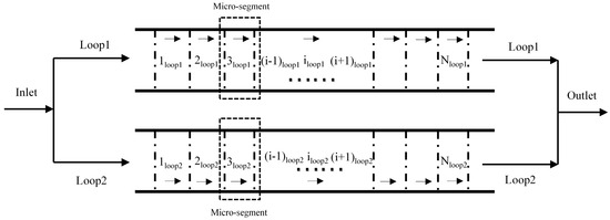
Figure 3. Simplified schematic diagram of the finite element method model [22]. The dotted horizontal line represents the boundary of the control region. The small black dots represent omissions. The dashed box represents a complete control region.

The discrete equations for the metal heat conduction equation are as follows. They are divided into a time term and a space term. Here, i represents the spatial node dimension, and t represents the time node dimension.

$$({\displaystyle \frac{\lambda }{\Delta \mathrm{x}}}+{\mathrm{h}}_1+{\displaystyle \frac{\rho \mathrm{c}\Delta \mathrm{x}}{3\Delta \tau }})T_1^{\mathrm{t}}+({\displaystyle \frac{\rho \mathrm{c}\Delta \mathrm{x}}{6\Delta \tau }}-{\displaystyle \frac{\lambda }{\Delta \mathrm{x}}})T_2^{\mathrm{t}}={\mathrm{h}}_1{T}_{\mathrm{a}1}+{\displaystyle \frac{\rho \mathrm{c}\Delta \mathrm{x}}{3\Delta \tau }}{T}_1^{\mathrm{t}-1}+{\displaystyle \frac{\rho \mathrm{c}\Delta \mathrm{x}}{6\Delta \tau }}{T}_2^{\mathrm{t}-1};$$

(18)

$$({\displaystyle \frac{\rho \mathrm{c}\Delta \mathrm{x}}{6\Delta \tau }}-{\displaystyle \frac{\lambda }{\Delta \mathrm{x}}})T_n^{\mathrm{t}}+({\displaystyle \frac{\lambda }{\Delta \mathrm{x}}}+{\mathrm{h}}_2+{\displaystyle \frac{\rho \mathrm{c}\Delta \mathrm{x}}{3\Delta \tau }})T_{n+1}^{\mathrm{t}}={\mathrm{h}}_2{T}_{\mathrm{a}2}^{\mathrm{t}}+{\displaystyle \frac{\rho \mathrm{c}\Delta \mathrm{x}}{3\Delta \tau }}{T}_{n+1}^{\mathrm{t}-1}+{\displaystyle \frac{\rho \mathrm{c}\Delta \mathrm{x}}{6\Delta \tau }}{T}_n^{\mathrm{t}-1};$$

(19)

$$({\displaystyle \frac{\rho \mathrm{c}\Delta \mathrm{x}}{6\Delta \tau }}-{\displaystyle \frac{\lambda }{\Delta \mathrm{x}}})T_{\mathrm{i}-1}^{\mathrm{t}}+({\displaystyle \frac{2\lambda }{\Delta \mathrm{x}}}+{\displaystyle \frac{2\rho \mathrm{c}\Delta \mathrm{x}}{3\Delta \tau }})T_{\mathrm{i}}^{\mathrm{t}}+({\displaystyle \frac{\rho \mathrm{c}\Delta \mathrm{x}}{6\Delta \tau }}-{\displaystyle \frac{\lambda }{\Delta \mathrm{x}}})T_{\mathrm{i}+1}^{\mathrm{t}}={\displaystyle \frac{\rho \mathrm{c}\Delta \mathrm{x}}{6\Delta \tau }}{T}_{\mathrm{i}-1}^{\mathrm{t}-1}+{\displaystyle \frac{2\rho \mathrm{c}\Delta \mathrm{x}}{3\Delta \tau }}{T}_{\mathrm{i}}^{\mathrm{t}-1}+{\displaystyle \frac{\rho \mathrm{c}\Delta \mathrm{x}}{6\Delta \tau }}{T}_{\mathrm{i}+1}^{\mathrm{t}-1},$$

(20)

where Δx is the spatial step size, Δτ is the temporal step size, and c is the specific heat capacity, t represents the current time step, and i represents the current spatial step.

The iterative solution process can be solved using the Gauss–Seidel iterative method. The energy equation is discretized using the first-order upwind difference method. After the difference operation, both the metal heat conduction equation and the energy equation are solved using the Gauss–Seidel iterative method. The essence of the equation is a system of linear equations of order n + 1 with n elements. Then, the metal wall temperature distributions at different spatial positions at different times are obtained by solving the matrix. The iterative formula of the Gauss–Seidel iterative method is:

$$T_{\mathrm{i}}^{(k+1)}={\displaystyle \frac{1}{a_{\mathrm{i},\mathrm{i}}}}(b_i-{\displaystyle {\sum }_{\mathrm{j}=1}^{\mathrm{i}-1}{a}_{\mathrm{i},\mathrm{j}}}{T}_{\mathrm{j}}^{(k+1)}-{\displaystyle {\sum }_{\mathrm{j}=\mathrm{i}+1}^{n+1}{a}_{\mathrm{i},\mathrm{j}}}{T}_{\mathrm{j}}^{\left(k\right)})\mathrm{i}=1,2,\dots ,n+1,$$

(21)

where k is the number of iterations. This iterative method utilizes both the k + 1 data during the iteration and the k data from the previous iteration, thus converging faster. Similar to most iterative methods, it requires initialization. In this way, the obtained temperature field is closer to the correct solution. That is, within the set error range, if the difference between two adjacent solutions is less than the set convergence value, it is determined that the obtained solution has converged to sufficient accuracy. At each time t, multiple iterations are needed to obtain an approximate solution of the temperature field at that moment, and then the solution at time t + 1 is obtained according to the equation. Therefore, during the solution process of each component, two iterative loops are required, namely the time loop for solving the transient term and the loop for the temperature field at each node at each moment. The solution processes of different models are approximately the same.

The SIMPLE algorithm is used to solve the velocity-pressure field. The number of velocity nodes is n, and the number of pressure nodes is n + 1. The specific solution process is as follows:

First, assuming an initial velocity distribution. Assume an initial velocity field and an initial pressure field for the system model with n nodes. Secondly, calculating the coefficients of the momentum equation. Calculate the coefficients and constant terms of the momentum discrete equation based on the velocity field and pressure field. Thirdly, solving the momentum equation. Discretize and solve the momentum equation to obtain a new velocity field. Fourth, solving the pressure correction equation. Solve the pressure correction equation according to the velocity field and correct the velocity and pressure. The entire solution logic involves a single solution process, which requires multiple iterative solutions. Determine whether the convergence condition is met. If not, continue the iterative solution.

The velocity-pressure field obtained by solving the momentum and mass equations using the SIMPLE algorithm and the temperature field are updated and iterated with each other, and finally, the solution of a model is completed.

In this paper, taking the solar collector as an example, the solution process of the single-component model is shown in Figure 4.

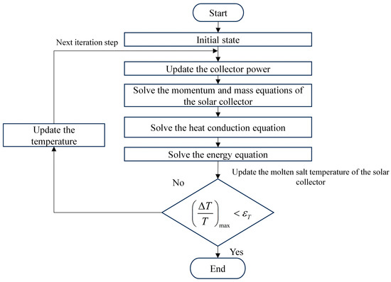
Figure 4. Transient solution process of the solar collector model.

2.2.2. Thermal Energy Storage System Model

The research object of the thermal energy storage system is the two-tank model. During the operation of the whole system, due to the influence of weather conditions and natural laws, the solar collector cannot maintain a highly efficient operating state for a long time. Therefore, the thermal energy storage system is required to play a buffering role. The two-tank storage method can store the molten salt working medium heated to the target temperature by the solar collector. At the same time, it can also transfer the molten salt working medium stored in the cold tank to the solar collector, ensuring the operation of the unit.

Its energy conservation equation is as follows, and the last term is the heat loss:

$${\displaystyle \frac{d{m}_{\mathrm{salt}}h}{dt}}=m_{\mathrm{salt}}{h}_{\mathrm{in}}-m_{\mathrm{salt}}{h}_{\mathrm{out}}+hA(T_{\mathrm{salt}}-T_{\mathrm{air}}),$$

(22)

where m_salt is the outlet flow rate of the hot molten salt. h_in and h_out are the enthalpy values at the inlet and outlet of the hot storage tank, respectively. T_air is the ambient temperature.

The mass conservation equation is expressed as Equation (23):

$${\displaystyle \frac{d{M}_{\mathrm{tank}}}{dt}}={\displaystyle \sum m_{\mathrm{tsnk},\mathrm{in}}}-{\displaystyle \sum m_{\mathrm{tank},\mathrm{out}}}.$$

(23)

The power of the entire thermal energy storage system can be expressed by Equation (24) [25]:

$$P_{\mathrm{ch}}=c_{\mathrm{f}}(m_1-m_2)(T_{\mathrm{hot}}-T_{\mathrm{cold}}).$$

(24)

The temperature field solution methodology of the heat storage tank model shares a common theoretical foundation with that of the solar collector model. The primary distinction resides in the treatment of the coupled flow and heat transfer mechanisms. Specifically, the heat storage tank model excludes the complex momentum conservation equations inherent in the solar collector model. The inlet and outlet of the heat storage tank are both regarded as flow boundaries. Based on this, the mass conservation equation is solved to obtain the flow distribution. Within each time step, the solution procedure for the heat storage tank model is illustrated in Figure 5.

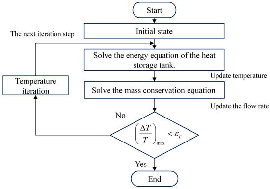
Figure 5. The solution procedure for the heat storage tank model is illustrated.

2.2.3. Intermediate Heat Exchanger Model

In this paper, the simulation object of the intermediate heat exchanger model is the PCHE. The calculation process mainly takes into account the convection and heat conduction models inside the regenerator. It is also assumed that the fluid in the pipeline is always in a stable state without phase change. The section where the cold fluid flows in is called the cold end of the heat exchanger, and the side where the hot fluid flows in is the hot end of the heat exchanger. The regenerator is divided into n nodes along the axial direction. At the same time, the heat transfer characteristics are calculated from the endpoints on each side, so as to calculate the state parameters of each node.

When calculating the heat exchanger in this paper, the heat exchanger is equivalent to a model with fluid channels on both sides and a metal heat-conducting layer in the middle. The calculated formulas for the cross-sectional area of the fluid and the heat-conducting area after modeling are as follows:

$$A=\left\{\begin{array}{c}{\displaystyle \frac{1}{1+R}}{N}_{\mathrm{c}}{N}_{\mathrm{p}}\left(\pi {D_{\mathrm{c}}}^2/8\right),\mathrm{cold}\\ {\displaystyle \frac{R_{\mathrm{p}}}{1+R}}{N}_{\mathrm{c}}{N}_{\mathrm{p}}\left(\pi {D_{\mathrm{c}}}^2/8\right),\mathrm{hot}\end{array}\right.;$$

(25)

$$A_{\mathrm{k}}={\displaystyle \frac{1}{1+R}}{N}_{\mathrm{c}}{N}_{\mathrm{p}}\left(1+{\displaystyle \frac{\pi }{2}}\right)D_{\mathrm{c}}{L}_{\mathrm{z}},$$

(26)

where d_e is the equivalent diameter, D_c is the diameter of the semi-circular flow channel, α is the included angle of the Z-shaped flow channel, L_z is the length of the regenerator core body, R is the ratio of the number of hot-side fluid plate layers to the number of cold-side fluid plate layers, N_p is the total number of hot-side and cold-side fluid plate layers, and N_c is the total number of flow channels on one layer of plate.

The energy conservation equations are expressed as Equations (27) and (28):

$${\displaystyle \frac{dm{h}_{\mathrm{hot}}}{dt}}=m_{\mathrm{in}}\left(h_{\mathrm{in}}-h_{\mathrm{out}}\right)-Q_{\mathrm{hot}};$$

(27)

$${\displaystyle \frac{dm{h}_{\mathrm{cold}}}{dt}}=m_{\mathrm{in}}\left(h_{\mathrm{in}}-h_{\mathrm{out}}\right)+Q_{\mathrm{cold}}.$$

(28)

Heat transferred from the molten salt to the metal wall and that transferred from the metal wall to the sCO₂ are:

$$Q_{\mathrm{hot}}=hA\left(T_{\mathrm{f},\mathrm{hot}}-T_{\mathrm{w},\mathrm{hot}}\right);$$

(29)

$$Q_{\mathrm{cold}}=hA\left(T_{\mathrm{w},\mathrm{cold}}-T_{\mathrm{f},\mathrm{cold}}\right).$$

(30)

In the heat conduction module, the change in the temperature of the metal solid can be expressed by Equation (31):

$$C_{\mathrm{w}}{M}_{\mathrm{w}}{\displaystyle \frac{d{T}_{\mathrm{w}}}{dt}}=Q_{\mathrm{hot}}-Q_{\mathrm{cold}},$$

(31)

where C_w is the specific heat capacity of the metal wall surface, and m_w is the mass of the metal wall surface.

The mass conservation equation and momentum conservation equation of the sCO₂ are:

$${\displaystyle \frac{dM}{dt}}={\displaystyle \sum m_{\mathrm{in}}}-{\displaystyle \sum m_{\mathrm{out}}};$$

(32)

$$\Delta P-\lambda {\displaystyle \frac{L}{d}}({\displaystyle \frac{\rho u^2}{2}})-\xi ({\displaystyle \frac{\rho u^2}{2}})-\rho gH={\displaystyle \frac{L}{A}}{\displaystyle \frac{\partial m}{\partial t}}.$$

(33)

The numerical calculation method for the molten salt side of the intermediate heat exchanger is the same as that of the solar collector. The energy and heat conduction equations are both solved using the Gauss iterative method, and the velocity and pressure are solved using the SIMPLE algorithm.

2.2.4. Valve Model

There are many types of valves. According to the flow characteristics, they can be classified as quick-opening valves, linear valves and percentage valves. Different characteristic curves have certain differences in system response. The calculation formulas of the valve model adopted in this paper are shown in Equations (34) to (37) [26]:

$$m_{\mathrm{out}}=m_{\mathrm{in}};$$

(34)

$$h_{\mathrm{out}}=h_{\mathrm{in}};$$

(35)

$$P_{\mathrm{out}}=P_{\mathrm{in}}-\Delta P;$$

(36)

$$m_{\mathrm{in}}=Af\sqrt{2\rho \Delta P},$$

(37)

where A represents the flow area, and f represents the valve opening. Under the condition that the pressures at both ends of the valve are the same, the flow rate of the valve is linearly distributed with the valve opening. However, since the valve is an indispensable component in the control system, the pressures at both ends of the valve and the physical parameters of the working medium will change. Therefore, in transient conditions, the valve opening and pressure changes need to be included in the iterative loop for processing.

2.3. Modeling Method for Brayton Cycle Side

In the Brayton cycle side, the sCO₂ fluid is treated as a homogeneous flow, and pipeline heat transfer losses to ambient are neglected. Fluid channels in components and pipelines are discretized into multiple control volumes, with mass and energy conservation equations derived for each control volume, as shown in Equations (38) and (39), respectively. The momentum conservation equation is formulated at the junction, as shown in Equation (40). These junctions are offset by half a spatial increment from the control volumes, according to the staggered grid method.

$${\displaystyle \frac{d{M}_i^{n+1}}{dt}}={\displaystyle \sum _{j\in T_i}{m}_j^{n+1}}-{\displaystyle \sum _{j\in I_i}{m}_j^{n+1}}+{\displaystyle \sum _{j>NEQ}{m}_j^n},(i=1,2,\dots ,NVOL);$$

(38)

$$\begin{array}{l}{\displaystyle \frac{d{U}_i^{n+1}}{dt}}=-{\displaystyle \frac{L_i}{2A_i}}{\left[{\displaystyle \frac{d}{dt}}\left({\displaystyle \frac{m_i^2}{{\rho }_i}}\right)\right]}^n+{\displaystyle \sum _{j\in T_i}{m}_j^{n+1}}\left\{h_j^n+{\displaystyle \frac{1}{2}}{\left[{\left({\displaystyle \frac{m_j}{{\rho }_i{A}_i}}\right)}^2\right]}^n+g\left(z_j-z_i\right)\right\}\\ -{\displaystyle \sum _{j\in I_i}{m}_j^{n+1}}\left\{h_j^n+{\displaystyle \frac{1}{2}}{\left[{\left({\displaystyle \frac{m_j}{{\rho }_i{A}_i}}\right)}^2\right]}^n+g\left(z_j-z_i\right)\right\}+{\displaystyle \sum _{j>NEQ}{m}_j^n{h}_j^n}+Q_i^n\end{array},$$

(39)

$$\begin{array}{l}{I}_j{\displaystyle \frac{d{m}_j}{dt}}={\displaystyle \frac{{\left(m_{Kcj}^2\right)}^{n+1}}{{\left({\rho }_K{A}_K^2\right)}^n}}-{\displaystyle \frac{{\left(m_{Lcj}^2\right)}^{n+1}}{{\left({\rho }_L{A}_L^2\right)}^n}}+{\displaystyle \frac{1}{2}}{\displaystyle \frac{{\left(m_j^2\right)}^{n+1}}{{\rho }_j}}\left[{\displaystyle \frac{1}{A_L^2}}-{\displaystyle \frac{1}{A_K^2}}\right]+{\left(p_K-p_L\right)}^{n+1}+P_{\mathrm{pump}}^n\\ +F_f^n\left|m_j^n\right|m_j^{n+1}-{\left({\displaystyle \frac{k_j}{2{\rho }_j{\left[A_j\left(t\right)\right]}^2}}\right)}^n\left|m_j^n\right|m_j^{n+1}-{\left({\displaystyle {\int }_K^j\rho dz}+{\displaystyle {\int }_j^L\rho dz}\right)}_g^n\end{array};$$

(40)

where ρ is the density with the unit of kg/m³. A is the area with the unit of m². m is the fluid flow rate with the unit of kg/s. p is the pressure with the unit of MPa. d is the equivalent diameter with the unit of m. f is the friction resistance coefficient. g is the acceleration due to gravity with the unit of m/s². U is the internal energy of the fluid with the unit of kJ/kg. h is the enthalpy value of the fluid with the unit of kJ/kg. Q is the internal heat source of the fluid with the unit of kW/kg. j is the number of nodes flowing into the current node. z is the node height. P_pump is the pressure source term.

By comparing with the molten salt side, the Brayton cycle side is solved using a simultaneous equation method, wherein the governing equations for all components are constructed as a matrix of joint equations, allowing the mass, momentum, and energy equations of entire cycle to be solved simultaneously. A generic fluid network modeling method is implemented to simultaneously solve the governing equations, enabling adaptation to Brayton cycles with various topological configurations. The fluid network model is described in Section 2.3.1. The component models of turbomachinery, PCHE heat exchanger, and constitutive models are described in Section 2.3.2, Section 2.3.3 and Section 2.3.4, respectively. The system solution strategy of the sCO₂ Brayton cycle side is illustrated in Section 2.3.5.

2.3.1. Fluid Network Model

In the fluid network model, links serve as the fundamental elements that define the connectivity relationships between control volumes [27]. The links can be divided into two categories: the critical link and the non-critical link, as depicted in Figure 6. Specifically, non-critical links, acting as coupling channels between internal nodes, have distinct starting and ending nodes, creating a two-way interaction between nodes. Critical links, functioning as the system’s boundary conditions, are defined only by their starting nodes and lack corresponding ending nodes. Essentially, they form the external environment’s input interface. The entire fluid network consists of a finite set of these two types of links.

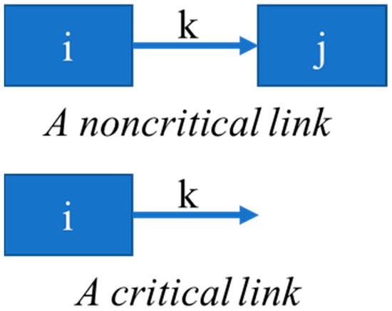
Figure 6. Schematic diagram of links. i represents the number of the starting region, j represents the number of the ending region, and k represents the number of the connection point.

A simple Brayton cycle is used here to further demonstrate the construction process of the fluid network. Figure 7 shows the discrete node diagram of the target system. In this figure, control volume 2 represents the gas turbine, node 3 is the control volume of the compressor, nodes 6 to 8 are the control volumes of the high-pressure side of the regenerator, nodes 13 to 15 are the control volumes of the low-pressure side of the regenerator, nodes 17 to 18 are the control volumes of the high-pressure side of the precooler, and nodes 21 to 23 are the control volumes of the low-pressure side of the precooler. The remaining nodes are the control volumes of the pipelines. It is worth noting that the long black strip between node 2 and node 3 is the rotating shaft.

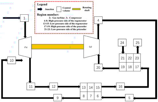
Figure 7. Schematic diagram of simple Brayton cycle nodes.

After the fluid grid of the system is determined, it needs to be re-encoded for subsequent calculations. The control volume at each node is divided into the starting control volume and the ending control volume. Two sets of indices, I_i and T_i, are used for re-encoding. T_i is the set of link indices with control volume i as the ending control volume, and I_i is the set of link indices with control volume i as the starting control volume. Therefore, the conservation equation at each node is divided into two parts, which are T_i and I_i. The fluid grid in Figure 7 is transformed into a matrix form as shown in Figure 8, where “X” represents non-zero terms.

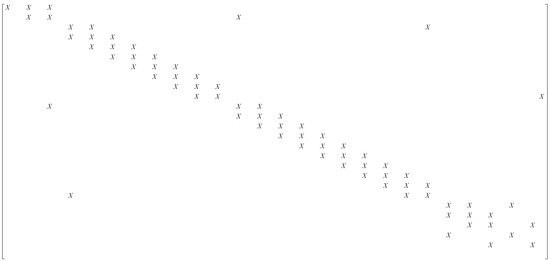
Figure 8. Structure of matrix A for the network of Figure 7.

2.3.2. Rotating Machinery Model

This section mainly explains how to solve different source terms for different components.

For solving turbomachinery (compressors and turbines) in the Brayton cycle, fluid changes within turbomachinery during the transient process are assumed to be in a quasi-static state. Based on this assumption, turbomachinery performance curves are used to interpolate and find the efficiency and pressure ratio of turbomachinery. When using the transient analysis program for solving, turbomachinery is treated as a junction and a node. The pressure rise (or drop) calculated from the pressure ratio acts on the momentum equation of the turbomachinery’s inlet junction. Meanwhile, the work done by the rotating shaft on the fluid inside turbomachinery, obtained through calculation, is added to the energy conservation equation of the turbomachinery’s fluid node as a source term.

When the fluid flows through the compressor, the following model will be adopted to calculate the node pressure change and energy change brought by the gas turbine machinery:

$$\Delta P=P_1^T\left(R_{\mathrm{p}}-1\right);$$

(41)

$$W_{\mathrm{c}.\mathrm{v}.}=m{\eta }_{\mathrm{ad}}\left(h_{2\prime }^T-h_1^T\right),$$

(42)

where ΔP is the pressure change in the rotating machinery. P₁^T is the total pressure at the inlet of the rotating machinery. R_p is the pressure ratio of the rotating machinery, which is obtained by querying the performance curve. W_c.v. is the work done by the rotating machinery on the fluid. m is the flow rate of the rotating machinery. η_ad is the adiabatic efficiency of the rotating machinery, which is obtained by querying the performance curve. $h_{2\prime }^T$ is the ideal enthalpy value at the outlet of the rotating machinery. $h_1^T$ is the enthalpy value at the inlet of the rotating machinery.

The working process of a gas turbine is the opposite of that of a compressor, but its pressure change and work can still be calculated using Equations (45) and (46). Physically, this means that the gas turbine consumes the fluid’s work, and the pressure rise is negative.

In the Brayton cycle, the gas turbine and the compressor are both connected to the same shaft. Therefore, it is necessary to calculate the rotational speed of the shaft:

$${\displaystyle \sum _i{I}_i}{\displaystyle \frac{d\omega }{dt}}={\displaystyle \sum _i^n{\tau }_i}+{\displaystyle \sum _{i=1}^n{f}_i}\omega +{\tau }_c,$$

(43)

where the first term on the right side represents the torque generated by the gas turbine and the compressor, the second term represents the torque generated by friction, and the last term is the torque of the control system. For the gas turbine and the compressor, the torque values generated by them are:

$${\tau }_{\mathrm{t}}={\displaystyle \frac{m{\eta }_{\mathrm{ad}}}{\omega }}\left(h_{2\prime }^T-h_1^T\right);$$

(44)

$${\tau }_{\mathrm{t}}={\displaystyle \frac{m}{\omega {\eta }_{\mathrm{ad}}}}\left(h_{2\prime }^T-h_1^T\right).$$

(45)

2.3.3. Heat Exchanger Model

The regenerator and precooler models on the Brayton cycle side are consistent with the intermediate heat exchanger on the molten salt side. Their equivalent cross-sectional areas and heat conduction heat exchange areas are also calculated by Equations (25) and (26), and their heat source term calculation formulas in the energy equation are shown in Equations (29) and (30).

The heat conduction equation on the Breton side is assumed to be a one-dimensional heat conduction equation, which is discretized using the finite difference method and solved by the Gauss–Seidel iterative method.

The nodes are divided into internal nodes and boundary nodes. The discrete format of the internal nodes is:

$$\left[{\left(\rho cV\right)}_{\mathrm{Li}}+{\left(\rho cV\right)}_{\mathrm{Ri}}\right]{\displaystyle \frac{T_{\mathrm{i}}^{n+1}-T_{\mathrm{i}}^n}{\Delta t}}={\lambda }_{\mathrm{Li}}{A}_{\mathrm{Li}}(T_{\mathrm{i}+1}-T_{\mathrm{i}})+{\lambda }_{\mathrm{Ri}}{A}_{\mathrm{Ri}}(T_{\mathrm{i}+1}-T_{\mathrm{i}})+Q_{\mathrm{Li}}+Q_{\mathrm{Ri}},$$

(46)

where the subscript Li represents the left control volume of node i, Ri represents the right control volume, the superscript n represents the time step, Δt is the time step size, and V indicates volume.

The discrete format of the left boundary is:

$${\left(\rho cV\right)}_{\mathrm{Ri}}{\displaystyle \frac{T_{\mathrm{i}}^{n+1}-T_{\mathrm{i}}^n}{\Delta t}}={\lambda }_{\mathrm{Ri}}{A}_{\mathrm{Ri}}(T_{\mathrm{i}+1}-T_{\mathrm{i}})+Q_{\mathrm{Ri}}+Q.$$

(47)

The discrete format of the right boundary is:

$${\left(\rho cV\right)}_{\mathrm{Li}}{\displaystyle \frac{T_{\mathrm{i}}^{n+1}-T_{\mathrm{i}}^n}{\Delta t}}={\lambda }_{\mathrm{Li}}{A}_{\mathrm{Li}}(T_{\mathrm{i}+1}-T_{\mathrm{i}})+Q_{\mathrm{Li}}+Q,$$

(48)

where Q is the boundary heat source.

2.3.4. Constitutive Models for Heat Transfer and Friction

The calculation of frictional resistance uses the correlations related to Zigrang-Sylvester [28]. This set of calculation methods is applicable to all flow regions on the carbon dioxide side of this system.

The calculation is divided into three regions based on the Reynolds number. When the Reynolds number is greater than 3400:

$${\displaystyle \frac{1}{\sqrt{f}}}=-2\log \left\{{\displaystyle \frac{\epsilon }{3.7D_e}}+{\displaystyle \frac{2.51}{\mathrm{Re}}}\left[1.14-2\log \left({\displaystyle \frac{\epsilon }{D_e}}+{\displaystyle \frac{21.25}{{\mathrm{Re}}^{0.9}}}\right)\right]\right\}.$$

(49)

When the Reynolds number is less than 2300:

$$f={\displaystyle \frac{64}{\mathrm{Re}}},$$

(50)

f is the frictional resistance coefficient.

In all the components currently designed, when dealing with regions involving heat exchange, it is necessary to calculate the convective heat transfer coefficient, which is generally calculated through the Nusselt number.

$$N_u={\displaystyle \frac{h{D}_e}{\lambda }}={\displaystyle \frac{\left(f/8\right)\left(\mathrm{Re}-1000\right)\mathrm{Pr}}{1+12.7\sqrt{\left(f/8\right)}\left({\mathrm{Pr}}^{2/3}-1\right)}},$$

(51)

$$f={\displaystyle \frac{1}{{\left(1.8\log \left(\mathrm{Re}\right)-1.5\right)}^2}}.$$

(52)

2.3.5. System Solution Strategy for Brayton Cycle Side

Based on the fluid network model established in Section 2.3.1, the joint matrix of all the conservation equations of each control volume and junction can be formulated, as shown in Equation (53):

$${\displaystyle \frac{d{Y}^{n+1}}{dt}}=f(Y^{n+1})+g\left(Y^n\right),$$

(53)

where Y represents internal energy, flow rate or mass.

The Gauss–Seidel iteration is employed to solve for the Jacobi matrix J. As a result, the mass increment, energy increment of each control volume, and the flow rate increment ΔY of each junction are obtained. Thus, the mass, energy of each node, and the flow rate of each junction at the next iteration step can be calculated. The calculations of the mass increment, energy increment, and flow rate increment ΔY are as follows:

$$\Delta Y=J^{-1}\cdot B$$

(54)

$$J=\left[\begin{array}{l}1-\Delta t\cdot \left({\left.{\displaystyle \frac{\partial f_1}{\partial Y_1}}\right|}_{Y^n}\right) ,-\Delta t\cdot \left({\left.{\displaystyle \frac{\partial f_1}{\partial Y_2}}\right|}_{Y^n}\right)\hspace{1em}\hspace{1em},\cdot \cdot \cdot \cdot \cdot \cdot \cdot \cdot \cdot \cdot -\Delta t\cdot \left({\left.{\displaystyle \frac{\partial f_1}{\partial Y_{2nv+nj}}}\right|}_{Y^n}\right)\\ -\Delta t\cdot \left({\left.{\displaystyle \frac{\partial f_2}{\partial Y_1}}\right|}_{Y^n}\right)\hspace{1em},1-\Delta t\cdot \left({\left.{\displaystyle \frac{\partial f_2}{\partial Y_2}}\right|}_{Y^n}\right)\hspace{1em},\cdot \cdot \cdot \cdot \cdot \cdot \cdot \cdot \cdot \cdot -\Delta t\cdot \left({\left.{\displaystyle \frac{\partial f_2}{\partial Y_{2nv+nj}}}\right|}_{Y^n}\right)\\ \cdot \cdot \cdot \cdot \cdot \cdot \cdot \cdot \cdot \cdot \cdot \cdot \cdot \cdot \cdot \cdot \cdot \cdot \cdot \cdot \cdot \cdot \cdot \cdot \cdot \cdot \cdot \cdot \cdot \cdot \cdot \cdot \cdot \cdot \cdot \cdot \cdot \cdot \cdot \cdot \cdot \cdot \cdot \cdot \cdot \cdot \cdot \cdot \cdot \cdot \cdot \cdot \cdot \cdot \cdot \cdot \cdot \cdot \cdot \cdot \cdot \\ -\Delta t\cdot \left({\left.{\displaystyle \frac{\partial f_{2nv+nj}}{\partial Y_1}}\right|}_{Y^n}\right),-\Delta t\cdot \left({\left.{\displaystyle \frac{\partial f_{2nv+nj}}{\partial Y_2}}\right|}_{Y^n}\right),\cdot \cdot \cdot \cdot \cdot \cdot \cdot \cdot 1-\Delta t\cdot \left({\left.{\displaystyle \frac{\partial f_{2nv+nj}}{\partial Y_{2nv+nj}}}\right|}_{Y^n}\right)\end{array}\right];$$

(55)

$$B=\left[\begin{array}{l}\Delta t\cdot \left(f_1\left(Y^n\right)+g_1\left(Y^n\right)\right)\\ \Delta t\cdot \left(f_2\left(Y^n\right)+g_2\left(Y^n\right)\right)\\ \cdot \cdot \cdot \cdot \cdot \cdot \cdot \cdot \cdot \\ \Delta t\cdot \left(f_{2nv+nj}\left(Y^n\right)+g_{2nv+nj}\left(Y^n\right)\right)\end{array}\right],$$

(56)

where Δt is the time step size, nv is the number of nodes, nj is the number of junctions, Yⁿ is the value of the independent variable at the current moment, and n represents the current moment.

The Brayton cycle side involves the overall solution of the entire system. The specific process is as follows: (i) Give the initial parameter distribution, solve the three major conservation equations to calculate the pressure distribution and temperature distribution of all control volumes in the system, and update the parameters of the junctions. (ii) The entire solution logic constitutes one solution process, and the solution process requires multiple iterative solutions. (iii) Determine whether the convergence condition is met. If it does not converge, continue the iterative solution. The solution logic is shown in Figure 9.

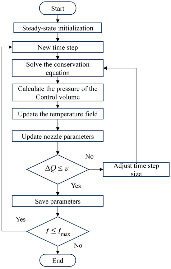
Figure 9. Breton side transient solution process.

2.4. Coupling Method for Molten Salt Side and sCO₂ Brayton Cycle Side

In this program, the molten salt side module is implemented using MATLAB S-functions, while the sCO₂ Brayton cycle module is developed in Fortran. It should be noted that the entire simulation is executed within the MATLAB/Simulink (version R2023b) environment. Therefore, to integrate the sCO₂ Brayton cycle module within the MATLAB/Simulink platform, the sCO₂ Brayton cycle code is compiled into a MEX file, which serves as an executable code within Simulink. The molten salt and Brayton systems are then coupled through an intermediate heat exchanger. To ensure proper coupling, essential data exchange between the two modules occurs at each time step, as illustrated in Figure 10.

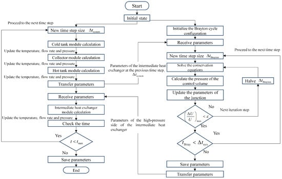
Figure 10. Flowchart of coupling system calculation.

When the simulation is initiated, both the molten salt module and the sCO₂ Brayton cycle module are invoked by Simulink. The molten salt module utilizes a time step identical to the global simulation time step configured in Simulink. In contrast, the sCO₂ Brayton cycle module employs an internal time step control logic. During each iteration, when Simulink calls the Brayton cycle module, the current global time step is also passed to it. The Brayton cycle module dynamically adjusts its internal time step based on thermal-hydraulic conditions, compares this value with the global time step received from Simulink, and selects the smaller of the two. The Brayton module’s computation proceeds through its internal time steps until it has advanced by one global Simulink time step. At this point, its computation ends, and the necessary data are transferred to the molten salt module. This approach ensures synchronization between the two modules.

The Brayton cycle side utilizes the outlet parameters of the high-pressure side of the intermediate heat exchanger at the previous time step as boundary conditions, and employs the rate of internal energy change as the convergence criterion during iteration, as shown in Equation (57). While the molten salt side utilizes the inlet parameters of the high-pressure side of the intermediate heat exchanger from the Brayton cycle module as boundary conditions, and employs the rate of temperature change as the convergence criterion. As shown in Equation (57), the convergence criterion is evaluated by assessing whether the relative change in energy between the current and next time steps remains within the specified tolerance. When the temperature residuals between two adjacent iteration steps meet the convergence conditions, it is considered that the system has reached a stable state:

$$\max \left\{\left[{\displaystyle \frac{T_i^{n+1}-T_i^n}{t^{n+1}-t^n}}-F_{T_i}\left(Y^{n+1}\right)\right]/{T^{n+1}}_i\right\}<\epsilon$$

(57)

To ensure the stability of the coupled numerical calculations, Simulink will automatically select the time step of the global simulation time step.

3. Results

3.1. Model Verification

3.1.1. PCHE Type Heat Exchangers Model Verification

In existing studies, the SCTRAN/CO₂ system program has been verified for components and the overall loop. For component verification, the compressor model was compared with experimental data from Bae et al. [29] and Fisher et al. [30] of the RELAP5 program. Also, by comparing the TRACE program’s [31] heat exchanger temperature distribution simulation results with the precooler outlet temperature experimental data [32], the stable heat exchanger and precooler models were verified. For the overall cycle, Wu et al. [33] confirmed the SCTRAN/CO₂’s dynamic prediction accuracy by comparing experimental data from a sudden reduction in cooling water flow rate with the system program.

To further boost the credibility of the SCTRAN/CO₂ system program in simulating the Brayton cycle side, a transient verification of the heat exchanger model was performed. To study the heat exchanger’s dynamic response characteristics during the transient process, Clementoni et al. [34] conducted a power transient operation experiment with a simple recuperated Brayton cycle at the Naval Nuclear Laboratory. Figure 11 presents the simulation and experimental results of the heat exchanger’s temperature and power during the transient process, where the electrical power rose from 5% to 30% in 12 s. The heat exchanger’s maximum temperature deviation is about 4.0 °C, and its power deviation is within 6%. This verifies SCTRAN/CO₂’s predictive ability for the heat exchanger’s transient behavior. Thus, it is deemed that this model’s transient simulation meets the research requirements of this paper.

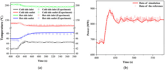
Figure 11. Transient verification of heat exchanger: (a) Comparison results of transient verification for heat exchanger temperature; (b) Comparison results of transient verification for heat exchanger power. Data of the reference come from reference [34].

3.1.2. Solar Collector Model Verification

On the solar thermal system side, the solar collector and the storage tank are two relatively critical models. In this paper, transient condition verifications are carried out on component models in the solar thermal system to demonstrate the models’ accuracy. Referring to the changes in the system’s temperature characteristics under different disturbances mentioned by Bai [35], a comparison is made with the models developed herein. The results are presented in Figure 12, which shows a comparative verification between the transient solar-side system model developed in this paper and the research of others.

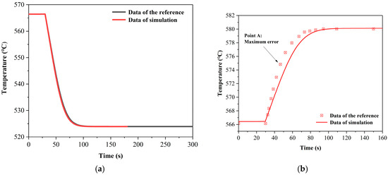
Figure 12. Transient verification of the solar collector model: (a) Comparison of collector outlet temperatures under reduced-load conditions; (b) Comparison of collector outlet temperatures under DNI disturbances. Point A: The location of the maximum error. Data of the reference come from reference [35].

The study object is the system with DNI and load disturbances at 30 s. Results show that during the DNI disturbance process, the maximum error compared with the work of Bai [35] is at point A in Figure 12b, with an error of 0.41%. When the system finally stabilizes, the error is 0.02%. Additionally, under the load-reduction condition, the difference between the solar collector’s outlet temperature and the simulation result is only 0.03%. Overall, the solar-side transient model is considered reliable.

3.1.3. Verification for Integrated System Simulation

For the integrated system, this paper selects the research of Zhang et al. [36] as the object for verification. The verified system diagram is shown in Figure 13. A comparative analysis was conducted on the system under two distinct operating conditions. A more comprehensive evaluation was performed to examine the system characteristics with inventory control implemented. Furthermore, a comparative verification was carried out for the same system under bypass control, under identical operating conditions, to enable a consistent assessment of performance differences.

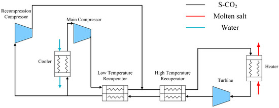
Figure 13. Diagram of the system to be verified.

At 200 s, the load was stepped down from 100% to 50% using inventory control. The load variation comparison chart, presented in Figure 14a, demonstrates a generally consistent trend with the experimental data. Discrepancies primarily arise following the disturbance event. As illustrated in Figure 14b, the maximum error in load variation reaches 1.88%, with a root mean square error (RMSE) of 0.2962 and an average relative error of 0.16%. The dynamic responses of the gas turbine outlet temperature and outlet pressure are illustrated in Figure 15a and Figure 16a. The results are presented in Figure 15b and Figure 16b. The maximum error for the gas turbine inlet temperature is 0.16%, with an RMSE of 0.2189, whereas the maximum error for the gas turbine inlet pressure reaches 1.21%, with an RMSE of 0.8294. The corresponding average relative errors are 0.03% and 0.32%, respectively.

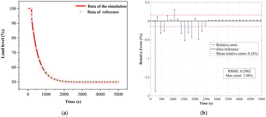
Figure 14. Program verification on system level under load variation scenario with inventory control method: (a) Comparison results of load level; (b) Relative error analysis of load level. Data of the reference come from reference [36].

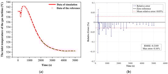
Figure 15. Program verification on system level under load variation scenario with inventory control method: (a) Comparison results of turbine inlet temperature; (b) Relative error analysis of turbine inlet temperature. Data of the reference come from reference [36].

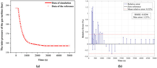
Figure 16. Program verification on system level under load variation scenario with inventory control method: (a) Comparison results of turbine inlet pressure; (b) Relative error analysis of turbine inlet pressure. Data of the reference come from reference [36].

In addition, under the condition of the same load step-down and using bypass control, as shown in Figure 17a. As shown in Figure 17b, for the integrated system applying bypass control, the maximum error of the gas turbine inlet temperature is 1.19%, the RMSE is 1.7179, and the average error is 0.14%.

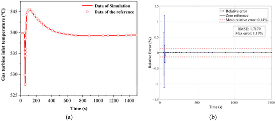
Figure 17. Program verification on system level under load variation scenario with bypass control method: (a) Transient verification of turbine inlet temperature; (b) Relative error analysis of turbine inlet temperature. Data of the reference come from reference [36].

Therefore, in conclusion, it is considered that the integrated system model established in this paper is accurate.

3.2. Dynamic Simulation Applications

This paper takes the SPT system with a simple regenerative cycle as the object for analyzing and verifying the transient analysis program. Through simulations of how load tracking and changes in solar irradiance affect the system characteristics, the performance and advantages of this transient analysis program are demonstrated.

The entire simulation process takes Simulink as the core operating interface and adopts a modular design for multi-physical field coupling. Specific operation steps are as follows: First, configure system design parameters in the solar-side module group. Then, enter the SCTRAN/CO₂ interface. There, users can select Brayton cycle configurations (like simple, reheat, or intercooled cycles) based on research needs and configure required output signal types (such as turbine power, heat exchanger temperature difference, system thermal efficiency). During the control signal input stage, specify time-series data of DNI, working fluid pressure conditions, mass flow rate adjustment curves, and other real-time control variables. After configuration, users define the simulation duration and step size in the time management module. Finally, execute the full-system simulation via the one-click start function of the Simulink interface.

3.2.1. Construction of the Simulation System Model

Figure 18 shows the Simulink-based schematic of the SPT system with a simple regenerative cycle. Inputs here are the intermediate heat exchanger’s cold-side output parameters (used by the SCTRAN/CO₂ system program for Brayton cycle calculation), system load input signals, and valve system input signals. Output parameters are the intermediate heat exchanger’s cold-side input parameters from the SCTRAN/CO₂ system program (for solar-side system calculation) and parameters like shaft speed. Table 3 shows the parameters of the SPT system and the Brayton cycle system.

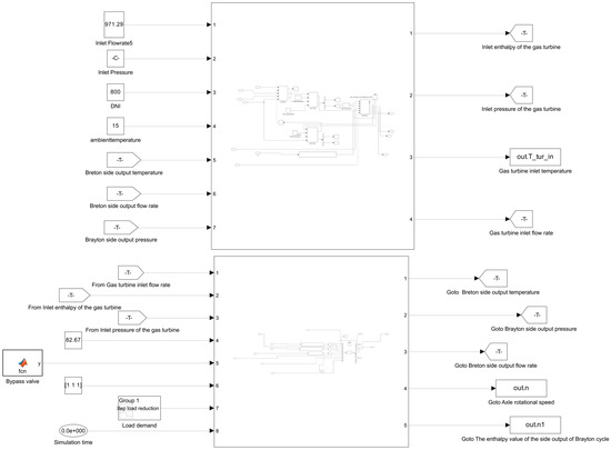
Figure 18. Schematic diagram of the solar thermal power generation system constructed in Simulink.

Table 3. Parameters of the SPT system with a simple regenerative cycle.

Item	Value
Number of heliostats, Nhel	4946
Length of heliostat, Lhel	12.0 m
Width of the heliostat, Whel	12.0 m
Mirror reflectance × Cleanliness, ρhel	0.9 × 0.97
Diameter of the receiver, Drec	15.0 m
Height of the receiver, Hrec	19.5 m
Number of pipes in each panel, Ntube	40
Outer diameter of pipe, dexternal	42.0 mm
Inner diameter of the pipe, dinternal	40.35 mm
Height of solar tower, Htower	220.0 m
Absorptivity of the receiver, αrec	0.94
Emissivity of the receiver, ηrec	0.85
Inlet pressure of the turbine	20.0 MPa
Inlet temperature of the turbine	550.0 °C
Compressor inlet pressure	9.04 MPa
Inlet temperature of the compressor	40 °C
The mass flow rate of the cycle	412.21 kg/s
Flow rate on the molten salt side	432.5 kg/s

3.2.2. Typical Results Under Dynamic Simulation

In the study of load disturbance’s impact on the system, firstly, the system’s response characteristics should be observed when turbine inlet temperature control is introduced. In investigating load disturbance effects on the SPT system, analyzing the gas turbine inlet temperature’s dynamic response characteristics is of great engineering significance. This study focuses on a temperature-controlled system. At 50 s, a 10% step reduction in rated load is imposed. Figure 19 shows the gas turbine inlet temperature’s dynamic response. The system features rapid load control and a short response time. After reaching peak parameter values, it gradually converges to the target temperature via the regulation mechanism. For the gas turbine inlet temperature, its stable margin is set to ±1 °C, the maximum temperature fluctuation is 9.2 °C, with an overshoot of 1.67%. The system enters the specified stability margin at 130 s, and the corresponding settling time is 80 s.

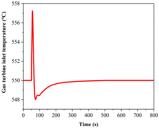
Figure 19. The response of the gas turbine inlet temperature to load step disturbances.

In actual operation, weather conditions greatly influence the SPT system. For instance, consider the sudden DNI drop due to cloud cover. We simulate the system’s controlled response characteristics under cloud influence by linearly reducing the DNI load in a short time. As the thermal storage system is designed in solar thermal power generation systems to stabilize operation and avoid the impact of sudden events, we observe the collector’s system characteristics during disturbances to check if the system can respond quickly and reach stability under special working conditions.

To investigate the system’s response to DNI disturbances, we simulate the condition of suddenly being covered by dark clouds. At this time, the solar irradiance received by the system drops from 800.0 MW/m² to 300.0 MW/m² within 30 s when the time is 300 s. The system’s response during this process is shown in Figure 20 and Figure 21.

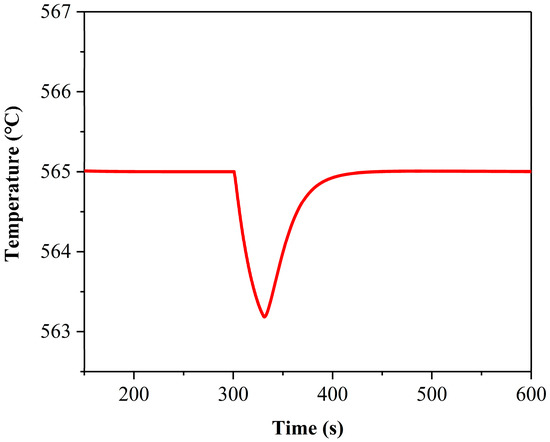
Figure 20. Dynamic response of solar collector outlet temperature when DNI disturbance is introduced into the system.

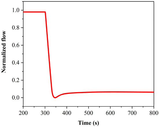
Figure 21. Dynamic response of solar collector outlet flow rate when DNI disturbance is introduced into the system.

Under the disturbance of DNI, the temperature response at the outlet of the collector shows typical dynamic regulation characteristics. When DNI undergoes a sudden change at 301 s, the outlet temperature begins to decline within 0.01 s. The temperature control system then actively intervenes by instantaneously reducing the system’s mass flow rate, effectively suppressing the rate of temperature drop. The stable margin of the collector inlet temperature is set to ±1 °C, and the stable margin of the normalized flow rate is set to ±0.25%. With the intervention of the temperature control system, the outlet temperature accurately reaches the target value at 446.64 s. The temperature overshoot is 0.32%. The maximum change is 1.81 °C. It enters the stable margin range at 350.16 s. The settling time is 50.16 s, and the peak time is 1.53 s. During this process, the mass flow rate reaches a steady state at 473.59 s. The setting time of the flow is 173.59 s, and the peak time is 46.23 s, completing the full transition from disturbance response to stable control.

Compared with the traditional quasi-steady-state analysis method, this program has notable advantages in dynamic characteristic analysis. Using high-precision time-domain simulation technology, it preserves the system’s transient response characteristics. Especially in complex models with closed-loop control systems, it can precisely describe the dynamic regulation process of the control strategy. This characteristic offers an integrated support platform for full-element dynamic modeling and control algorithm verification in the solar thermal power generation field.

4. Discussion

First, the program development method is discussed as follows. Considering the trade-off between computational time consumption and simulation accuracy, a one-dimensional transient modeling approach is adopted to describe the system’s flow and heat transfer processes. Under the operating conditions considered in the validation and application cases of this study, the CO₂ working fluid remains in a supercritical state, allowing the use of a single-phase flow model. However, to account for potential two-phase flow phenomena under extreme conditions—such as the compressor inlet entering the two-phase region during load-following operation, or phase change and gas–liquid two-phase flow occurring during some coolant leakage accidents—a homogeneous flow model is adopted in this program to calculate thermal-hydraulic parameter variations, thereby enhancing the code’s extensibility for future research. Furthermore, to address the inherent flexibility in sCO₂ cycle configurations and account for the impact of actuators (e.g., bypass valves, inventory tanks) on cycle topology during control strategy studies, a generic fluid network model is implemented. This approach characterizes the connectivity of discrete nodes within the Brayton cycle, thereby achieving the requirement for simultaneous solution of all governing equations for arbitrary topological configurations using the current numerical solution strategy. Furthermore, to reduce code development complexity, an external coupling approach is implemented between the Brayton and molten salt loops.

Second, the capability of the program is discussed based on the results presented in Section 3. Section 3.1 indicates that the program can qualitatively capture the transient trends of key performance parameters for both the integrated system and its components during transitions induced by variations in boundary conditions (e.g., load, DNI). The initial verification results on the integrated system level indicate that the transient prediction accuracy for key cycle parameters is within 5%. This confirms the effectiveness of the program’s fluid model and the molten salt/sCO₂ Brayton loop coupling method. Furthermore, in comparison to quasi-steady-state models, the transient model provides more detailed information on component temperatures, pressures, flow rates, and power levels during transient responses. These parameters are critical for controller design, control strategy study, and safety analysis. Section 3.2 employs a typical load and DNI disturbance scenario to demonstrate the program’s application in the field of control strategy study. When modifications to components such as recuperators, compressors, gas turbines, valves, and inventory tanks are required due to changes in Brayton cycle topology or control strategies, these adjustments can be implemented by simply modifying the input card settings. The program can be integrated with the SIMULINK platform, where the power plant’s controller model can be constructed, thereby facilitating convenient modeling for studies on control strategies and safety analysis for the integrated system.

Finally, the limitations of the current program and potential directions for future work are discussed. (a) Due to the lack of enough data on large-scale or experimental integrated systems, the verification on the integrated system level was only conducted with experimental data from Zhang et al. [36]. Furthermore, the available parameters from the literature are limited to system load and turbine inlet temperature/pressure. This results in relatively limited validation data for the integrated system, with few parameters available for verification. Future work will focus on acquiring additional transient validation data for the integrated system to further enhance the program’s reliability. Additionally, uncertainty quantification could be performed to assess the impact of different models or parameters on the program’s computational accuracy, thereby providing guidance for future model modification. (b) The simulation results under some extreme conditions should be treated carefully. For instance, if the molten salt temperature exceeds 580 °C during transients, decomposition may occur. The program does not account for the effects of salt decomposition on fluid flow and heat transfer in the solar collector. As another example, although the CO₂ physical property parameters allow predictions within 0.1–25 MPa operating conditions and the conservation equations incorporate a two-phase flow model, the accuracy of results during transcritical Brayton cycle operation requires careful consideration. This caution is warranted because the program has not been validated under transcritical conditions and does not employ appropriate constitutive models (e.g., critical flow, friction, and heat transfer models) for such scenarios. (c) Although the program can simulate CSP systems integrated with various Brayton cycle configurations, it has certain limitations regarding the solar field layout and Brayton cycle cooling methods. For the solar side, the use of a sequential solution method requires solving the conservation equations for each component in a specific order based on the cycle topology. Consequently, the program is currently limited to the solar field layout depicted in Figure 1. Modifications to the solar field layout would require optimization of the cycle solution strategy. For the Brayton cycle side, only water cooling is currently implemented. The absence of constitutive models for air prevents the performance prediction for Brayton cycles employing the air-cooling method. The program can be readily enhanced for air-cooling applications by implementing additional physical property models and heat transfer/friction correlations for air, without requiring modifications to the Brayton cycle solution module. Given the fact of the advantages of air cooling in arid regions, this represents a critical direction for future program enhancement.

5. Conclusions

A one-dimensional transient analysis tool for solar power tower (SPT) systems integrated with sCO₂ Brayton cycles has been developed, utilizing the staggered grid method, lumped parameter method, and one-order upwind difference scheme. Verification at both component and integrated system levels, along with transient simulations of load and DNI variation scenarios for a CSP integrated system, has been conducted to confirm the program’s capabilities. The main conclusions are as follows:

(a)

Thermodynamic analysis for CSP integrated system based on transient model can supply more detailed information about the transition process than quasi-steady state models, which is essential for controller design and safety analysis.

(b)

The fluid network model adopted in this program enables a universal representation of discrete node connectivity relationships for various configurations, thereby providing the foundation for simultaneous solution of all governing equations within a Brayton cycle and consequently achieving predictive capability for arbitrary Brayton cycle layouts without modifications for cycle solution strategy.

(c)

Verification results and transient simulations conducted in this study demonstrate the program’s capability to predict transient responses in CSP integrated systems. With prediction errors for key parameters within 2%, the program meets the requirements for dynamic characteristic analysis, controller design, control strategy development, and safety assessment.

(d)

Future work should be focused on transient validation with more integrated system operations and model uncertainty quantification to enhance prediction accuracy and reliability. Additionally, implementing constitutive models for air will extend the program’s predictive capability to dry cooling applications.

References

- Jiang, T.; Liu, Z.; Wang, G.; Chen, Z. Comparative study of thermally stratified tank using different heat transfer materials for concentrated solar power plant. Energy Rep. 2021, 7, 3678–3687. [Google Scholar] [CrossRef]
- Wang, G.; Zhang, Z.; Chen, Z. Design and performance evaluation of a novel CPV-T system using nano-fluid spectrum filter and with high solar concentrating uniformity. Energy 2023, 267, 126616. [Google Scholar] [CrossRef]
- Wang, G.; Liu, J. Design and performance evaluation of a novel photovoltaic and concentrated solar thermal system using parabolic trough-shaped spectrum filter. Energy Source Part A Recovery Util. Environ. Eff. 2025, 47, 6918–6933. [Google Scholar] [CrossRef]
- Wang, G.; Chao, Y.; Jiang, T.; Chen, Z. Facilitating developments of solar thermal power and nuclear power generations for carbon neutral: A study based on evolutionary game theoretic method. Sci. Total Environ. 2022, 814, 151927. [Google Scholar] [CrossRef]
- Wang, G.; Hao, J.; Wang, B.; Han, W. Comparative study on thermal and mechanical performances of liquid lead thermocline heat storage tank with different solid filling material layouts. Case Stud. Therm. Eng. 2025, 73, 106754. [Google Scholar] [CrossRef]
- Wang, G.; Zhang, S.; Zou, T. Design and comparison study of a novel linear Fresnel reflector solar ORC-driven hydrogen production system using different working fluids. Case Stud. Therm. Eng. 2025, 71, 106187. [Google Scholar] [CrossRef]
- Wang, G.; Li, D.; Zou, T.; Duan, Y. Design and performance evaluation of an innovative solar concentration polygeneration system. Renew. Energy 2025, 251, 123441. [Google Scholar] [CrossRef]
- Abdelghafar, M.M.; Hassan, M.A.; Kayed, H. Direct integration of supercritical carbon dioxide-based concentrated solar power systems and gas power cycles: Advances and outlook. Appl. Therm. Eng. 2025, 269, 126064. [Google Scholar] [CrossRef]
- Li, H.; Zhang, R.; Li, Z.; Lee, S.; Ju, Y.; Zhang, C.; Lu, Y. Design optimization and off-design performance analysis of one-dimensional supercritical CO2 Brayton cycle. Appl. Therm. Eng. 2025, 258, 124547. [Google Scholar] [CrossRef]
- Soumhi, M.; Zalim, Y.; Ahmadi, Z.E.L.; Hamdani, F.E.L.; Bouzekri, H. Comparative study of supercritical CO2 Brayton cycles for solar towers plants in arid climates: Design and off-design performance. Energy Convers. Manag. 2025, 337, 119902. [Google Scholar] [CrossRef]
- Zhai, R.; Chen, Y.; Li, J.; Du, M.; Yang, Y. Intelligent construction and optimization based on the heatsep method of a supercritical CO2 Brayton cycle driven by a solar power tower system. Sol. Energy Mater. Sol. Cells 2024, 276, 113075. [Google Scholar] [CrossRef]
- Li, C.; Tao, Y.B.; Li, S.; Dang, K. Performance optimization of high-temperature supercritical carbon dioxide concentrating solar power plant with an improved solar receiver. Energy Convers. Manag. 2025, 336, 119883. [Google Scholar] [CrossRef]
- Jiang, T.; Li, M.; Wang, W.; Li, D.; Liu, Z. Fluid-thermal-mechanical coupled analysis and optimized design of printed circuit heat exchanger with airfoil fins of S-CO2 Brayton cycle. J. Therm. Sci. 2022, 31, 2264–2280. [Google Scholar] [CrossRef]
- Battisti, F.G.; Klein, C.F.; Escobar, R.A.; Cardemil, J.M. Exergy Analysis and Off-Design Modeling of a Solar-Driven Supercritical CO2 Recompression Brayton Cycle. Energies 2023, 16, 4755. [Google Scholar] [CrossRef]
- Lu, Q.; Zhao, J.; Fang, S.; Ye, W.; Pan, S. Investigation of thermodynamics of the supercritical CO2 Brayton cycle used in solar power at off-design conditions. Sustain. Energy Technol. Assess. 2022, 52, 102361. [Google Scholar] [CrossRef]
- Chen, K.Q.; Pu, W.H.; Zhang, Q.; Lan, B.-S.; Song, Z.-Y.; Mao, Y.-Q. Thermal performance analysis on steady-state and dynamic response characteristic in solar tower power plant based on supercritical carbon dioxide Brayton cycle. Energy Source Part A Recovery Util. Environ. Eff. 2025, 47, 1927–1949. [Google Scholar] [CrossRef]
- Yu, Q.; Yang, Y.; Xu, X.; Shi, B.; Xiong, X.; Li, Z.; Wu, Z.; Yang, Z.; Fang, Z. Modeling and dynamic characteristics analysis of concentrating-receiver-heat exchanger system of sCO2 solar thermal power plant. Sol. Energy Mater. Sol. Cells 2025, 282, 113341. [Google Scholar] [CrossRef]
- Delsoto, G.S.; Battisti, F.G.; Da Silva, A.K. Dynamic modeling and control of a solar-powered Brayton cycle using supercritical CO2 and optimization of its thermal energy storage. Renew. Energy 2023, 206, 336–356. [Google Scholar] [CrossRef]
- Wang, D.; Han, X.; Li, H.; Li, X. Dynamic simulation and parameter analysis of solar-coal hybrid power plant based on the supercritical CO2 Brayton cycle. Energy 2023, 272, 127102. [Google Scholar] [CrossRef]
- Wang, G.; Zhang, Z.; Lin, J. Multi-energy complementary power systems based on solar energy: A review. Renew. Sustain. Energy Rev. 2024, 199, 114464. [Google Scholar] [CrossRef]
- Zou, Q. Research and Design on Heat Transfer Characteristics of Tower Solar Molten Salt Absorber. Master’s Thesis, Zhejiang University, Zhejiang, China, 2014. [Google Scholar]
- Yu, Q.; Fu, P.; Yang, Y.; Qiao, J.; Wang, Z.; Zhang, Q. Modeling and parametric study of molten salt receiver of concentrating solar power tower plant. Energy 2020, 200, 117505. [Google Scholar] [CrossRef]
- Hu, N. Research on Optimal Design and Focusing Strategy of the Concentrating and Heat Collecting System of a Tower Solar Thermal Power Station. Master’s Thesis, Zhejiang University, Zhejiang, China, 2020. [Google Scholar]
- Hojjat, M.; Etemad, S.G.; Bagheri, R.; Thibault, J. Turbulent forced convection heat transfer of non-Newtonian nanofluids. Exp. Therm. Fluid Sci. 2011, 35, 1351–1356. [Google Scholar] [CrossRef]
- Li, H. Research on Modeling and Simulation of Heat Transfer and Energy Storage System for Tower Solar Thermal Power Generation. Master’s Thesis, North China Electric Power University, Beijing, China, 2019. [Google Scholar]
- Ding, H. Transient Simulation and Control of Supercritical Carbon Dioxide Brayton Cycle. Master’s Thesis, Xiamen University, Fujian, China, 2021. [Google Scholar]
- Porsching, T.A.; Murphy, J.H.; Redfield, J.A. Stable numerical integration of conservation equations for hydraulic networks. Nucl. Sci. Eng. 1971, 43, 218–225. [Google Scholar] [CrossRef]
- Fang, X.D.; Xu, Y.; Zhou, Z.R. New correlations of single-phase friction factor for turbulent pipe flow and evaluation of existing single-phase friction factor correlations. Nucl. Eng. Des. 2011, 241, 897–902. [Google Scholar] [CrossRef]
- Bae, S.J.; Ahn, Y.; Lee, J.; Kim, S.G.; Baik, S.; Lee, J.I. Experimental and numerical investigation of supercritical CO2 test loop transient behavior near the critical point operation. Appl. Therm. Eng. 2016, 99, 572–582. [Google Scholar] [CrossRef]
- Fisher, J.E.; Davis, C.B.; Weaver, W.L. RELAP5-3D Compressor Model; Idaho National Laboratory (INL): Idaho Falls, ID, USA, 2005.
- Hexemer, M.J.; Hoang, H.T.; Rahner, K.D.; Siebert, B.; Wahl, G.D. Integrated systems test (IST) S-CO2 Brayton loop transient model description and initial results. In Proceedings of the Supercritical CO2 Power Cycle Symposium 2009, Troy, NY, USA, 30 April 2009. [Google Scholar]
- Van Meter, J. Experimental Investigation of a Printed Circuit Heat Exchanger Using Supercritical Carbon Dioxide and Water as Heat Transfer Media. Ph.D. Thesis, Kansas State University, Manhattan, KS, USA, 2008. [Google Scholar]
- Wu, P.; Gao, C.; Shan, J. Development and verification of a transient analysis tool for reactor system using supercritical CO2 Brayton cycle as power conversion system. Sci. Technol. Nucl. Install. 2018, 2018, 6801736. [Google Scholar] [CrossRef]
- Clementoni, E.M.; Cox, T.L.; King, M.A. Response of a compact recuperator to thermal transients in a supercritical carbon dioxide Brayton cycle. In Proceedings of the Turbo Expo: Power for Land, Sea, and Air American Society of Mechanical Engineers, Charlotte, NC, USA, 26–30 June 2017. [Google Scholar]
- Bai, X. Modeling and Dynamic Analysis of Tower-Type Solar Collectors. Master’s Thesis, North China Electric Power University, Beijing, China, 2018. [Google Scholar]
- Zhang, J.; Yang, Z.; Le Moullec, Y. Dynamic modeling and transient analysis of a molten salt heated recompression supercritical CO2 Brayton cycle. In Proceedings of the 6th International Supercritical CO2 Power Cycles Symposium 2018, Pittsburgh, PA, USA, 27– 29 March 2018. [Google Scholar]
Disclaimer/Publisher’s Note: The statements, opinions and data contained in all publications are solely those of the individual author(s) and contributor(s) and not of MDPI and/or the editor(s). MDPI and/or the editor(s) disclaim responsibility for any injury to people or property resulting from any ideas, methods, instructions or products referred to in the content. |
© 2025 by the authors. Licensee MDPI, Basel, Switzerland. This article is an open access article distributed under the terms and conditions of the Creative Commons Attribution (CC BY) license (https://creativecommons.org/licenses/by/4.0/).