GA-LSTM-Based Degradation Prediction for IGBTs in Power Electronic Systems

Abstract

The reliability and lifetime of insulated gate bipolar transistors (IGBTs) are critical to ensuring the stability and safety of power electronic systems. IGBTs are widely used in electric vehicles, renewable energy systems, and industrial automation. However, their degradation over time poses a significant risk to system performance. Therefore, this paper proposes a data-driven approach based on a Long Short-Term Memory (LSTM) network optimized by a Genetic Algorithm (GA) to predict IGBT degradation. The study examines the health monitoring of insulated gate bipolar transistors from a device physics perspective. Degradation mechanisms that alter parasitics and electro-thermal stress produce characteristic changes in the turn-off overvoltage and the on-state voltage. Using power-cycling data from packaged half-bridge modules, an LSTM-based sequence model configured by a genetic algorithm search reduces error against an identically trained baseline (RMSE = 0.0073, MAE = 0.057, MAPE = 0.726%) under the shared protocol, with the clearest advantages in the early stage of degradation. These results support predictive maintenance and health management in power-electronic systems.

1. Introduction

Insulated gate bipolar transistors (IGBTs) are key components in power electronic systems and are widely deployed in electric vehicles, renewable energy systems, industrial automation, and consumer electronics [1,2]. Their main features include high efficiency, low saturation voltage, high current density, and simple drive control, which make them central to modern power applications. However, the performance of IGBTs gradually degrades over time. Under high current and high switching frequency, thermal and mechanical stresses accumulate, altering measurable electrical quantities such as the collector-to-emitter voltage and the gate-to-emitter voltage. The resulting drift increases the risk of system failure and unplanned downtime. Despite advances in packaging and thermal management, failures remain possible. Early prediction of degradation trends, accurate estimation of remaining useful life, and timely fault warnings are therefore essential for safe and reliable operation.

Existing approaches to IGBT degradation prediction can be categorized into three main groups: physical modeling, statistical reliability modeling, and data-driven modeling. Physical modeling relies on stress–strain and thermo-mechanical analyses to describe internal mechanisms. Complex material properties and variable operating conditions limit its accuracy. For example, Ahsan [3] studied the impact of switching frequency and power loss on IGBT reliability, while Li [4] and Wang [5] reported physics-based models for battery aging. Although theoretically rigorous, these models often show limited generalization due to material heterogeneity and unpredictable environments, which has reduced interest in purely physical approaches. Statistical modeling uses historical failure data and lifetime distributions. Thebaud et al. applied Weibull distributions to predict IGBT damage levels [6], and Zio et al. combined particle filtering and Monte Carlo simulation in a Bayesian framework to assess battery health [7]. However, methods grounded in reliability statistics depend on probability density fitting and may yield insufficient accuracy when data are scarce or heterogeneous.

Data-driven methods have emerged as a promising alternative because they capture complex degradation patterns directly from measurements [8]. Neural networks, in particular, have shown potential. Ahsan [9] developed models based on neural networks and adaptive neuro-fuzzy inference systems; however, their performance was limited at the early stage of degradation. Ismail et al. [10] proposed a feed-forward neural network with principal component analysis and reported a prediction accuracy of 60.4%. To better model temporal dependence, recurrent neural networks and their variants have been introduced. Reference [11] utilized the collector-to-emitter conduction voltage as a feature for an LSTM-based remaining life prediction model, demonstrating that the early trend can be captured and updated as aging progresses. Xie Feng [12] proposed a GRU-based model that handles changing operating conditions. In practice, data-driven approaches can learn latent degradation patterns from large datasets. Nevertheless, conventional neural networks still struggle in the early stage, where feature changes are subtle. Additionally, selecting LSTM architectures and hyperparameters can be computationally expensive, which limits their practical deployment [13]. Recent work on physics-informed machine learning (PIML) formalizes how domain knowledge can regularize learning objectives and architectures in prognostics and health management. Surveys from 2023 and 2024 summarize integration patterns, including physics-guided feature construction, constrained losses, and hybrid gray-box structures, for condition monitoring, and highlight the benefits under small-data regimes, along with deployment considerations [14,15,16,17]. This literature provides the broader context for device-centric IGBT prognostics and motivates the use of lightweight physics checks alongside data-driven forecasting.

Recent studies have explored optimized LSTM variants for predicting IGBT health. CNN-LSTM combines convolutional layers for spatial correlations with LSTM layers for temporal dynamics, which is helpful for multivariate inputs and has shown promise in tracking IGBT aging under varying conditions [18]. EMD-LSTM utilizes empirical mode decomposition to extract intrinsic mode functions from nonlinear, non-stationary signals, and then feeds them to an LSTM to enhance accuracy for complex waveforms [19]. LSTM-AE integrates autoencoding into LSTM to learn compact representations when labeled data are limited, which can help detect early degradation [20]. Convolutional-LSTM augments LSTM with convolutional feature extraction for scenarios that involve both spatial and temporal structure, as in multi-sensor configurations [21]. Related optimization and learning strategies, such as improved swarm-based algorithms and gray-code-inspired search for feature selection and model tuning, have been reported in broader machine learning contexts and motivate automated model configuration for predictive maintenance [22,23].

Although these models provide value, many require manual architecture design and extensive tuning. This paper proposes a practical alternative for IGBT degradation forecasting: an extended short-term memory network configured through a simple, budgeted genetic algorithm search. The search selects depth and width within a predefined space by validation loss under a shared protocol. The focus of the study is not a new optimizer. The contribution is an IGBT-specific formulation that links failure mechanisms to measurable indicators and then to forecasting suitable for maintenance planning. Bond-wire and solder-layer fatigue progressively modify the current path, parasitics, and thermal state. During fast turn-off with a high current fall rate, these changes appear as a larger and more variable turn-off overvoltage. In contrast, during conduction, the on-state collector-to-emitter voltage (denoted $V_{CE,on}$) reflects the evolution of temperature and the conduction path. These indicators are measurable in power-cycling experiments and motivate short, cycle-aligned input windows. All models in this work employ identical preprocessing, normalization based on the training set, device-stratified splits, and a consistent window length to ensure reproducibility and fair comparison.

The remainder of the paper is organized as follows. Section 2 summarizes the IGBT structure and failure mechanisms, explaining the link between these mechanisms and observables. Section 3 describes the dataset, indicator extraction, and construction of cycle-aligned inputs. Section 4 presents the forecasting model and the validation-based search used to set its configuration. Section 5 presents the results and discusses robustness, runtime, and improvements to figures and captions. Section 6 concludes and outlines directions for multivariate indicators and hybrid physics-informed modeling.

2. IGBT Failure Analysis

2.1. IGBT Structure

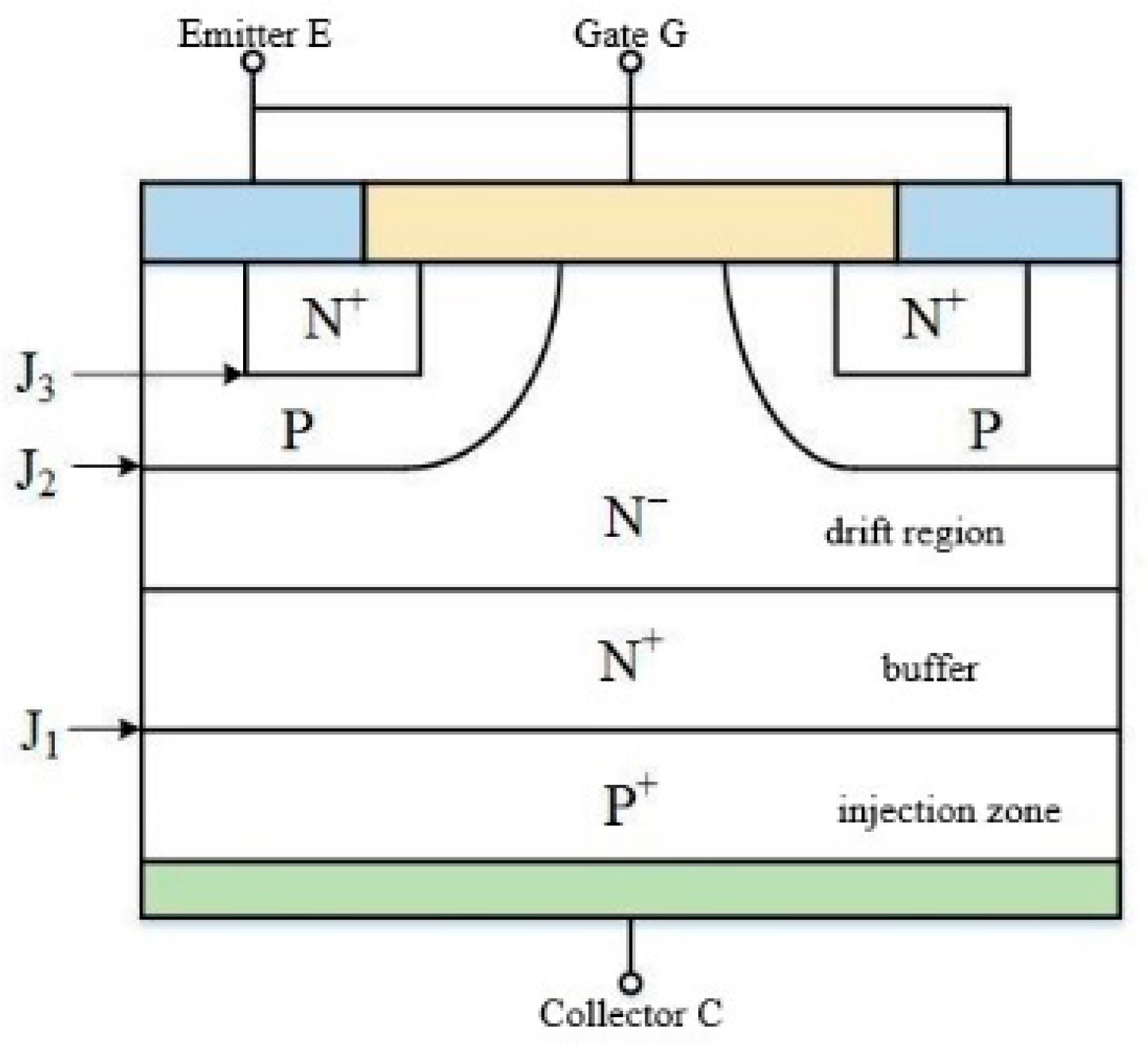
Insulated gate bipolar transistors integrate a voltage-controlled MOS gate with a conductivity-modulated bipolar conduction path, as shown in Figure 1. This combination enables fast switching while minimizing conduction loss, supporting applications in electric vehicles, renewable energy converters, and industrial motor drives. First, consider the layered structure. A typical device comprises a p⁺ collector, an n⁻ drift region, a p-base, and an n⁺ emitter. The polysilicon gate is insulated from the semiconductor by a thin oxide. When the gate-to-emitter voltage (denoted $V_{GE}$) exceeds the threshold, an inversion channel forms in the p-base and injects carriers into the n⁻ drift region. Conductivity modulation in this region allows a large collector current at a moderate on-state voltage. Many modern devices employ trench gates, field-stop layers, and optimized cell pitches to balance conduction loss and switching behavior. Second, consider the operating states. IGBTs operate in reverse blocking, forward blocking, turn-on, and turn-off modes. In forward blocking, the drift region sustains the applied voltage. In turn-on, a voltage above the threshold creates the channel and establishes a conduction path from the collector to the emitter. In turn-off, removing the gate drive extinguishes the channel, and the device returns to the blocking state. The charge stored in the drift region decays during this transition, shaping the switching waveform. Third, relate structure to performance. The thickness and doping of the n⁻ drift region set the blocking capability and contribute to on-state loss. The p⁺ collector and lifetime control affect carrier storage and the tail current observed during turn-off. Gate structure and cell density influence channel resistance and switching loss. These design choices determine key performance indicators such as breakdown voltage, conduction loss, and switching speed. Finally, connect the structure to the degradation indicators. Device structure and its interconnects couple to measurable electrical quantities during power cycling. Changes in interconnects and interfaces modify parasitics and the electro-thermal state, which appear as a variation in the turn-off overvoltage on the collector-to-emitter (denoted $V_{CE}$) path. In contrast, the $V_{CE,on}$ reflects the evolution of the conduction path and temperature. Understanding the structure, therefore, provides the basis for analyzing degradation mechanisms and for selecting practical indicators for forecasting in later sections.

Figure 1. Structure of IGBT.

2.2. Failure Mechanism

In practical applications, IGBTs are assembled as packaged power modules, as shown in Figure 2a. Differences in thermal conductivity and coefficients of thermal expansion across the multilayer stack produce temperature gradients during operation. The resulting thermo-mechanical stress is cyclic under switching and load variation and accumulates into fatigue damage over time [13,24]. Bond-wire degradation is a primary failure mechanism. Concentrated stress at the wire heel and bond interface promotes the initiation of microcracks, interfacial degradation, and eventual lift-off. These changes increase local resistance and modify loop parasitics, which affect the switching waveform. Observable consequences include drift in the $V_{CE,on}$ and larger, more variable turn-off overvoltage [25]. Solder-layer degradation is another dominant mechanism. Voids, crack growth, and partial delamination raise the effective thermal resistance of the joint and facilitate local hot spots. The altered electro-thermal state perturbs conduction voltage and the turn-off waveform, and it can accelerate damage in neighboring regions [26]. These mechanisms may interact. Increased thermal resistance due to solder damage amplifies the temperature swing at the bond interface, while bond-wire degradation intensifies current crowding within the solder joint. The indicators analyzed in the later sections are chosen to reflect these structural changes during power cycling, with an emphasis on the turn-off overvoltage and the $V_{CE,on}$.

Figure 2. Package structure of IGBT module and failure mark (a) schematic diagram of the package structure of the IGBT module (b).

2.3. Physics Observable Coupling in IGBT Degradation

Degradation in bond wires and solder layers increases loop inductance and series resistance and shifts the electro-thermal operating point. During fast turn-off with a high current fall rate, the resulting inductive overvoltage produces a larger and more variable collector-to-emitter turn-off waveform with a characteristic ring-down. During conduction, the $V_{CE,on}$ tracks changes in the conduction path and temperature. This linkage from mechanism to observable motivates the selection of turn-off overvoltage and $V_{CE,on}$ as practical indicators, and it supports the use of short, cycle-aligned inputs for forecasting and health thresholding, with particular sensitivity to the early stage of degradation. Thermo-mechanical analysis shows that voiding in the solder layer raises junction temperature and effective thermal resistance, increasing electro-thermal stress at turn-off and thus elevating the peak collector-to-emitter turn-off overvoltage; this evidence substantiates the mechanism-to-observable mapping used here [27].

Device-level studies indicate that coupling basic electro-thermal consistency with recurrent models can stabilize early-stage models by discouraging non-physical trajectories. A physics-informed recurrent approach for discrete power devices demonstrates that incorporating monotonicity and boundary conditions into the loss function improves out-of-sample error on the NASA IGBT dataset. Complementary IGBT work leverages waveform-derived health indicators in conjunction with a recent multiscale transformer architecture, yielding strong descriptive accuracy on accelerated aging data. These results are consistent with using measurable, turn-off-centered indicators and provide a path to add simple constraints within our short-window forecasting pipeline.

Recent thermo-mechanical studies quantify the pathway from structural damage to measurable waveform changes [27] report that voids in the solder layer increase junction temperature and that the rise grows with void radius, is strongest when the void is near the layer center or top corner, and increases with void density; they also show a near-linear dependence on solder-layer thickness (about 0.8 °C per 0.025 mm) and a reduction in peak temperature when nanosilver solder is used (e.g., ≈5% improvement in their setup). Elevated junction temperature and higher effective thermal resistance strengthen electro-thermal stress during fast turn-off, which appears as a larger and more variable peak collector-to-emitter turn-off voltage, denoted $V_{CE,p}$. Complementarily [28], use flow–solid coupling to show that cooling-channel geometry and fin design shape the device thermal field through the series thermal-resistance path from junction to coolant, implying that indicator stability for $V_{CE,p}$ and the conduction-phase $V_{CE,on}$ depends on local cooling conditions. These results are consistent with our choice of $V_{CE,p}$ as the primary observable and $V_{CE,on}$ as a complementary measure, and they motivate event-centered, turn-off-aligned inputs for forecasting.

3. Aging Dataset and Feature Parameter Selection

Accurately predicting IGBT degradation requires the acquisition of high-quality aging datasets and well-defined feature parameters. This section details the source of the aging dataset, the feature selection process, and the rationale for the selection of feature parameters used in predictive modeling.

3.1. Source of Aging Dataset

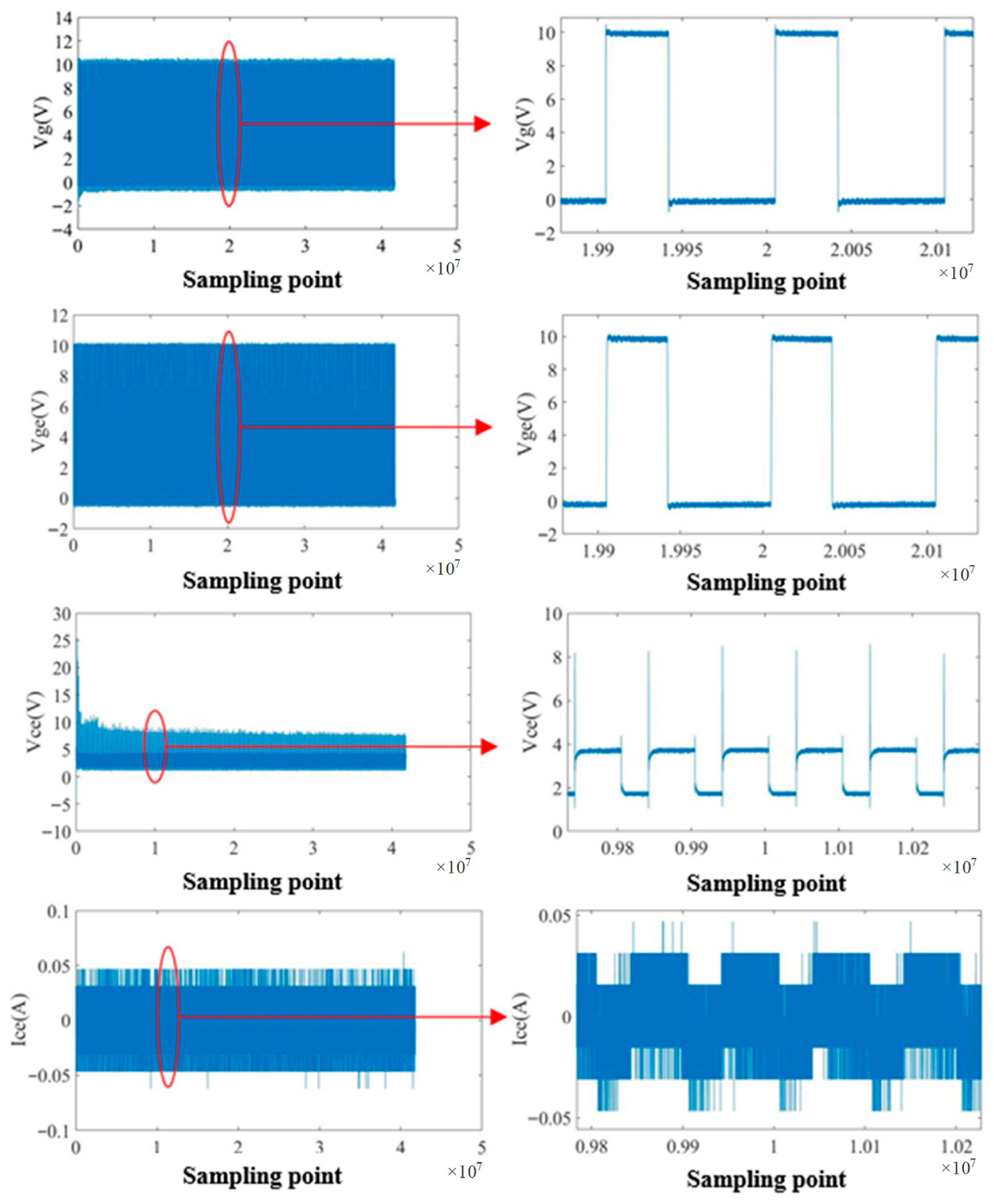
This study uses the NASA Prognostics Center of Excellence IGBT Accelerated Aging Data Set (original release 2009) for packaged half-bridge IGBT modules (type YBTM600F07) [29]. The repository description documents aging data from six devices, with one device aged under DC gate bias and the remainder under a squared-signal gate bias, and includes high-speed measurements of gate voltage, collector–emitter voltage, and collector current.

Power-cycling experiments are conducted under controlled conditions to accelerate degradation, using a gate-drive frequency of 10 kHz and a PWM duty cycle of 40%. Junction-temperature setpoints range from 329 to 345 °C. The test sequence lasts about 170 min until latch failure and yields 418 transient switching records. Each cycle contains 100,000 samples that include gate voltage, $V_{GE}$, $V_{CE}$, and collector current. Waveforms are processed to extract two indicators used throughout this study: the turn-off overvoltage and the $V_{CE,on}$. A cycle-aligned sliding window constructs input sequences, and a simple window-based augmentation generates 5- to 20-step variants to mitigate overfitting and represent short-term fluctuations. The train, validation, and test partitions are stratified by device and operating condition to prevent leakage. Normalization statistics are computed on the training set and then applied to the validation and test sets. Table 1 summarizes the operating settings for the power-cycling experiments, and Figure 3 presents representative switching records. Table 1 shows a fixed 10 kHz gate drive and a 40% duty cycle across conditions, with junction temperatures set between 329 and 345 °C. The settings accelerate degradation while maintaining consistent acquisition, so models are compared under the same preprocessing and windowing conditions. Figure 3 shows cycle-aligned waveforms with clear turn-off events and sufficient sampling density. The records preserve cycle-to-cycle variability, which supports the extraction of the turn-off overvoltage and the $V_{CE,on}$ for forecasting. The window-based augmentation preserves cycle alignment and label semantics, does not alter the class of operating conditions, and prevents device-level information from leaking across the train/validation/test splits.

Table 1. Operating conditions for IGBT power-cycling experiments (NASA PCoE).

Parameter	Value
Supply voltage (V)	4
Gate drive voltage (V)	10
Low set-point temperature (°C)	329
High set-point temperature (°C)	330
Protection threshold temperature (°C)	345
PWM duty cycle	40%
Switching frequency (kHz)	10

Figure 3. Cycle-aligned switching records with identifiable turn-off events.

3.2. Selection and Processing of Failure Characteristic Parameters

Degradation of internal structures in IGBT modules produces gradual changes in measurable electrical quantities. Indicator choice, therefore, focuses on signals that are sensitive to early deterioration and practical to obtain in power cycling. Two indicators are used throughout: turn-off overvoltage and $V_{CE,on}$. The former responds to parasitic and electrothermal shifts around the turn-off event, the latter tracks conduction path and temperature evolution. A five-point cubic smoothing removes high-frequency fluctuations while preserving the global trend. Time-series inputs are built by a cycle-aligned sliding window centered on the turn-off event. Window lengths of 5, 10, 15, and 20 steps are evaluated under identical preprocessing. Short windows emphasize local transients and better capture incipient changes, whereas longer windows introduce noise accumulation and reduce the number of usable sequences for a dataset of about 850 training samples. This trade-off is evident in the window study, where the 20-step setting yields a higher error than the 5-step setting (for example, RMSE 0.405 for 20 steps). All inputs are min-max normalized to the range [0, 1] using the training set statistics.

The same smoothing, cycle-aligned windowing, normalization, and device-stratified splits apply across all models. These steps stabilize indicator extraction, preserve local transients near the turn-off event, and prevent leakage between devices and operating conditions. In addition to the primary indicator, the framework allows for the inclusion of $V_{CE,on}$, gate-to-emitter threshold voltage when measurable, and a thermal-resistance proxy derived from the transient thermal response. These quantities are concatenated into a multivariate, cycle-aligned window under the same normalization and splits. This construction preserves the protocol while providing complementary information for stability under fluctuating conditions.

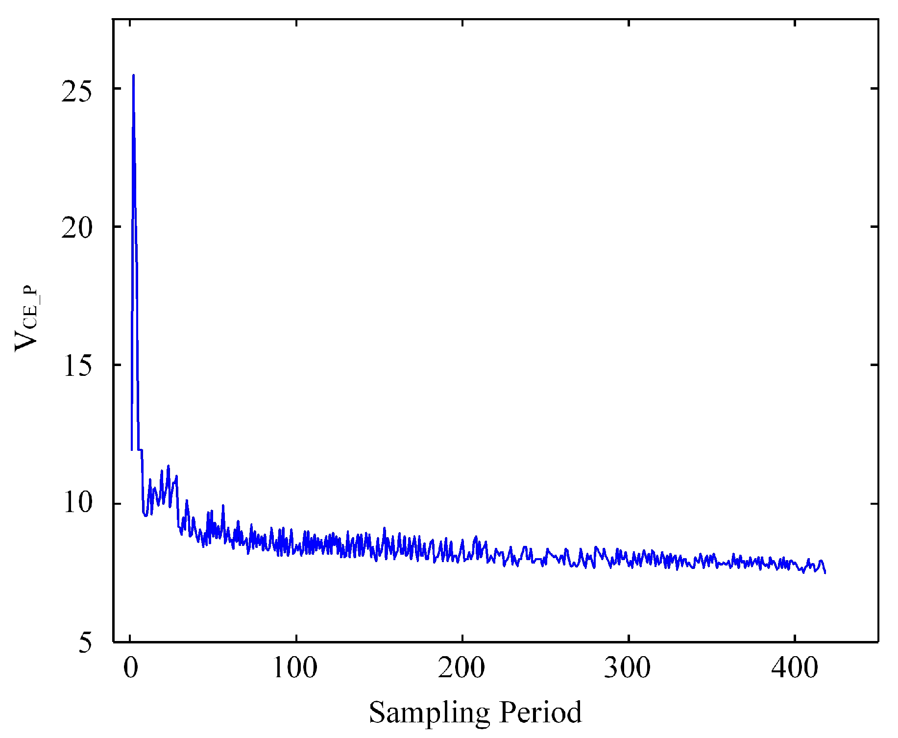
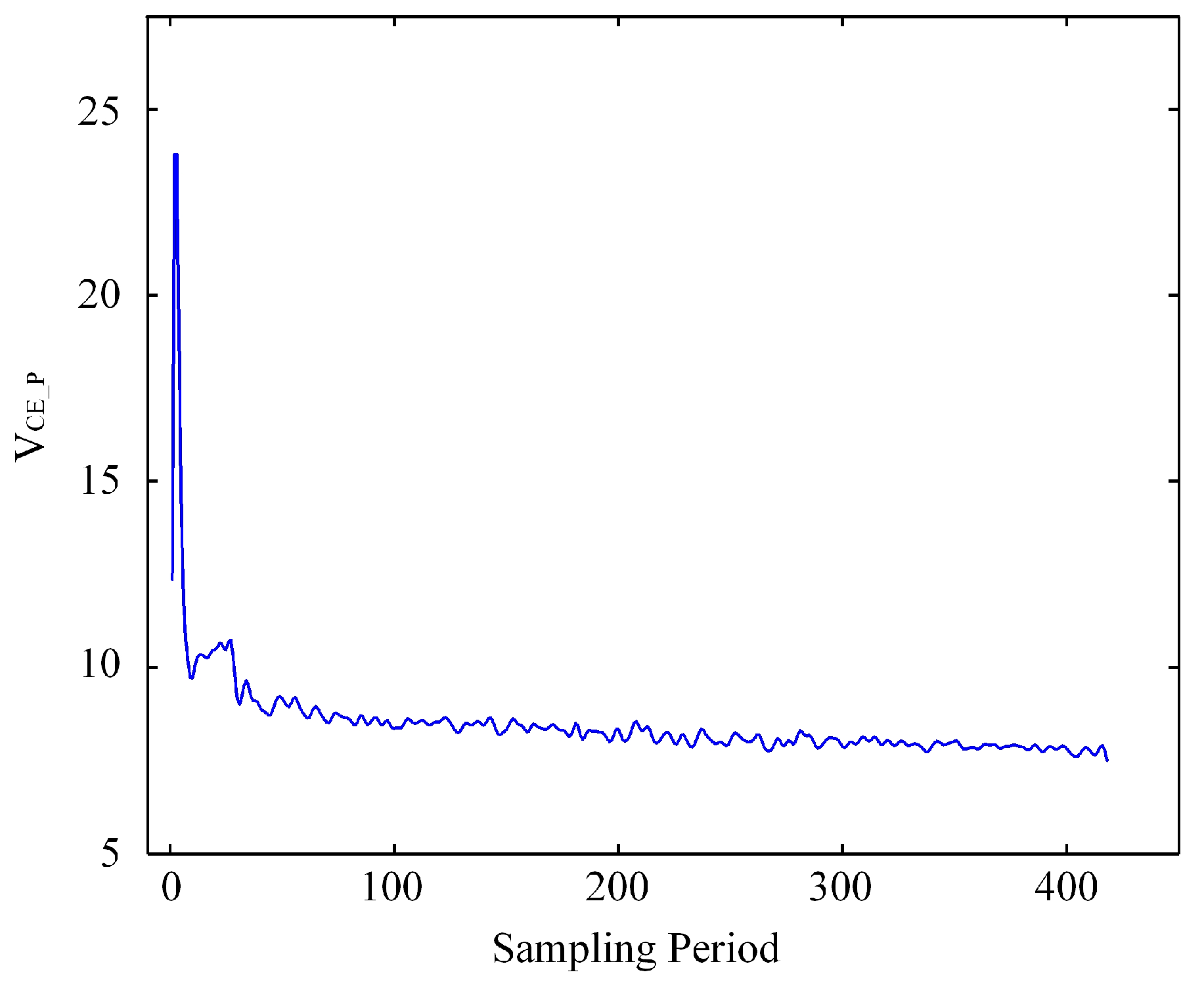
A long short-term memory (LSTM) architecture is employed to model the short, cycle-aligned sequences. Network depth and hidden-unit width are selected by a genetic algorithm search within a predefined space, using validation loss under the shared protocol described in Section 4.3. The baseline uses a single-layer LSTM with a dense output. The GA-selected configuration increases capacity within bounds and is used for subsequent experiments under an identical evaluation protocol. As shown in Figure 4, the trajectory of the turn-off overvoltage versus cycle index. The global trend is monotonic with mid-term fluctuations, which supports the use of event-centered windows for forecasting. Figure 5 illustrates the effect of five-point cubic smoothing. Short-term noise is reduced while the overall tendency is preserved, which stabilizes indicator extraction and input construction.

Figure 4. Peak collector-to-emitter turn-off overvoltage $V_{CE,p}$ (V) vs. cycle index (cycles).

Figure 5. Smoothed trajectory of $V_{CE,p}$ (V) vs. cycle index (cycles).

In summary, the turn-off overvoltage serves as the primary indicator, complemented by smoothing, normalization, and cycle-aligned windowing. These preparations provide consistent inputs to the GA-tuned LSTM, emphasizing the early stage of degradation that is most relevant for maintenance.

4. GA-LSTM Prediction Model

Accurately predicting IGBT degradation requires a prediction model that can capture long-term dependencies in time series data and optimize model parameters to improve prediction accuracy. To achieve this, this study proposes an LSTM model optimized by a GA. This section provides a detailed description of the LSTM model’s working principle and the GA optimization process, accompanied by comprehensive flowcharts and diagrams.

4.1. LSTM Principle

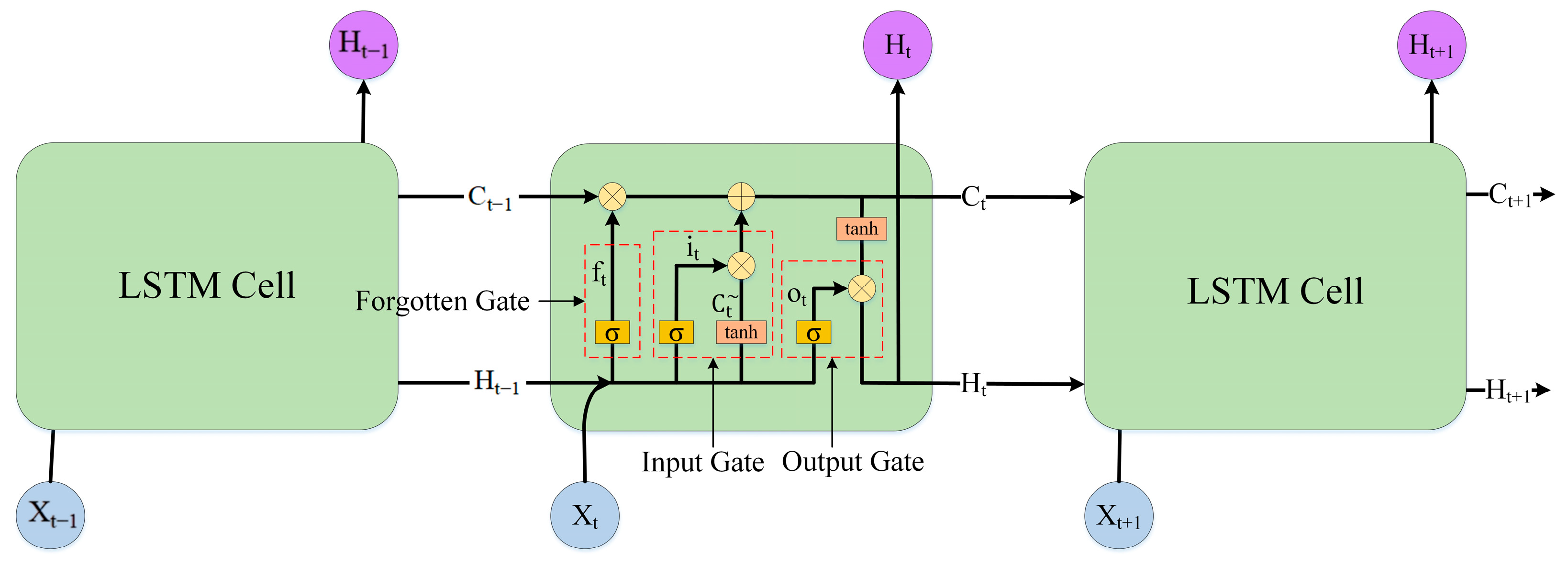
LSTM networks are a special type of recurrent neural network (RNN) designed to overcome the vanishing and exploding gradient problems that typically affect RNNs during long-term sequence modeling. The LSTM structure consists of three main components: the forget gate, the input gate, and the output gate. These components work together to selectively retain or discard information as data propagates through time steps. The structure of an LSTM cell is shown in Figure 6.

Figure 6. Structure of the LSTM cell.

Forgetting stage: long-term and short-term memory unit data from the previous moment $C_{t-1}$, $H_{t-1}$ and the input data $X_t$ at that time enters the unit structure together, and then filters through the forgetting gate important information in $C_{t-1}$. Forgotten Gate $f_t$ can be expressed as:

$$f_t=\sigma (W_f·\left[H_{t-1},X_t\right]{ + b}_f)$$

(1)

The input-gate operation determines which information from the candidate input is written to the cell state.

Information update stage: through input gate $i_t$ processes the short-term memory unit data $H_{t-1}$ of the previous moment and the input data $X_t$. Determine which information is stored in the long-term memory unit. Before the input gate operates, the current input and the previous hidden state are first passed through a tanh layer to form the candidate input. The input gate and the candidate input are then given by (2) and (3).

$$i_t=\sigma (W_i·\left[H_{t-1},X_t\right]{+b}_i)$$

(2)

$$C_t^{\sim }=\mathrm{t}\mathrm{a}\mathrm{n}\mathrm{h}(W_c·\left[H_{t-1},X_t\right]{+b}_c)$$

(3)

Through $i_t\times C_t^{\sim }$ operation determines which information in the input data is stored. After determining the information that needs to be forgotten and stored, the data of the long-term memory unit is updated. This process can be represented by Equation (4):

$$C_t=f_t\times C_{t-1} + i_t\times C_t^{\sim }$$

(4)

Output stage: Data based on long-term memory units passes through output gate $O_t$ determine final output, output gate $O_t$ and this process can be represented as:

$$O_t= \sigma (W_o·\left[H_{t-1},X_t\right]{ + b}_o)$$

(5)

$$H_t=O_t\odot \mathrm{t}\mathrm{a}\mathrm{n}\mathrm{h}\left(C_t\right)$$

(6)

where $\odot$ denotes element-wise multiplication between the output gate and the cell activation. By using forget gates, input gates, and output gates, LSTM can selectively remember important information while discarding irrelevant data. This makes LSTM an ideal choice for predicting time series data with long-term dependencies.

4.2. Integration of GA and LSTM

The Genetic Algorithm (GA) is a widely used optimization technique that mimics the natural process of survival of the fittest [13]. GA is well-suited to discrete or mixed search spaces, does not require gradients, and is less prone to getting trapped in local minima. It is easy to parallelize, works under a fixed compute budget, and provides a reproducible way to discover strong configurations. This work proposes a GA-LSTM prediction model for forecasting IGBT degradation. The choice is motivated by two constraints of the problem: the architectural space is discrete and modest in size, and the dataset is limited with a fixed evaluation budget. Under these conditions, the automatic selection of depth and width by a genetic algorithm provides a reproducible and straightforward method for configuring the forecaster. At the same time, all preprocessing, cycle-aligned inputs, and device-stratified splits remain identical to those used for the baselines. The goal is to achieve a configuration that matches short, event-centered sequences without altering the shared protocol.

The model combines an LSTM forecaster with a GA search over a predefined architecture space. Each candidate network is encoded as a chromosome that records the number of LSTM layers, the number of hidden units per layer, the number of dense layers, and the number of neurons in each dense layer. Feasible ranges are specified in advance to reflect implementable designs. The search considers one to three LSTM layers with 10 to 50 units per layer and one to three dense layers with 10 to 50 neurons. The budget uses a population of 40 and 20 generations, with a crossover probability of 0.5 and a mutation probability of 0.05. These settings strike a balance between exploration and computational cost on this dataset. For a given chromosome, the corresponding network is trained under the same normalization, cycle-aligned window length, early-stopping rule, and device-stratified train, validation, and test splits. Fitness is the validation loss computed on the shared validation set. Selection adopts tournament sampling; crossover exchanges architectural fields; mutation perturbs one field within its allowed range. After the fixed number of generations, the best configuration, as determined by validation loss, is retrained on the training set and then evaluated once on the test set without further adjustment.

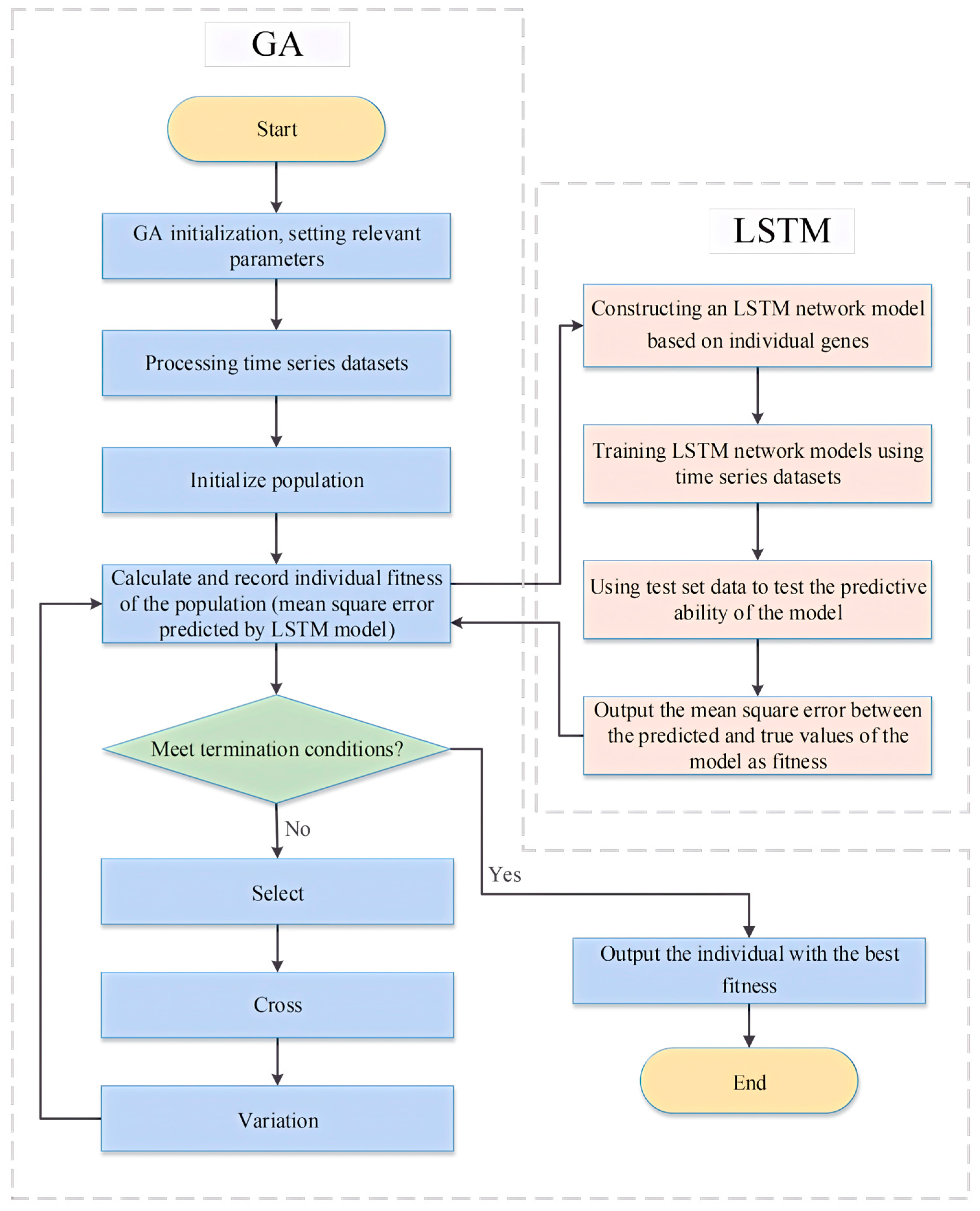
Compared to a plain LSTM tuned by hand, GA-LSTM eliminates the guesswork about depth and width, reducing the risk of over- or under-parameterization on a small dataset. The baseline LSTM in this study consists of one recurrent layer with 20 units and a single-neuron dense output; all other elements of preprocessing and evaluation remain the same, isolating the effect of architectural selection. The final GA-selected configuration, two LSTM layers with 40 units per layer, reflects a compromise between capacity and robustness under noisy, limited data. Table 2 records the architectural ranges for LSTM and GA-LSTM, along with the GA budget and baseline settings, allowing for configuration and capacity to be traced under the shared protocol. Figure 7 summarizes the workflow from population initialization to fitness evaluation and population update, explicitly stating that selection depends only on validation loss, while test data are not used. The detailed step sequence is provided in Appendix A. The role of the GA here is configurational rather than methodological. Alternatives, such as particle swarm optimization or Bayesian optimization, could operate in the same architectural space, but they are outside the present scope. Reported results should be interpreted within the context of this fixed-budget, validation-based protocol.

Table 2. Hyperparameters of the LSTM and GA-LSTM models.

Parameter	LSTM	GA-LSTM
Number of LSTM Layers	1	1–3
Neurons in Each LSTM Layer	20	10–50
Number of Dense Layers	1	1–3
Neurons in Each Dense Layer	1	10–50
Maximum Training Iterations	2000	4000
Population Size (GA)	-	40
Maximum Generations (GA)	-	20
Crossover Rate (GA)	-	0.5
Mutation Rate (GA)	-	0.05

Figure 7. Flowchart of GA optimized LSTM.

The forecaster operates on a short window of scalar or low-dimensional indicators. Let $L$ denote the input window length, $D$ the input dimension (e.g., $D=1$ for $V_{CE,p}$ alone, or small $D$ if auxiliary indicators are used), and $H$ the number of units in each LSTM layer selected by the GA. A single forward pass requires on the order of $O$ ($L{H}^2+LHD$) multiply–accumulate operations, plus a small output head. Under the configurations selected in this study and the short windows evaluated, the parameter count and compute scale linearly with $L$ and quadratically with $H$. These properties make per-sequence inference lightweight relative to data acquisition and feature extraction.

4.3. Baseline Models: Provenance, Tuning, and Disclosure

All experiments follow a shared protocol: identical preprocessing, cycle-aligned input windows, and device-stratified train, validation, and test splits. Normalization statistics are computed on the training set and applied to the validation and test sets. Model selection relies exclusively on validation loss on the shared validation split, and test data are not used for selection. Early stopping with a fixed patience is used where applicable. Model selection is performed on the validation set under this shared protocol. Test data are not used for selection. For readers implementing the physics-informed extension, Section 5.5 specifies how electro-thermal consistency terms can be added to the loss while keeping preprocessing, cycle-aligned windowing, device-stratified splits, and validation-based selection unchanged.

For transparency, Table 3 reports, for each baseline, the implementation provenance, the training budget, the validation-based selection rule, and the final hyperparameters that produced the results in Section 5.3. Parameter counts are also listed to indicate model capacity.

Table 3. Baseline configurations used in comparisons.

Model	Implementation/Provenance	Shared Protocol Settings	Final Hyperparameters (As Used)	Training Budget	Input Window	Training Time	Memory Usage
CNN-LSTM	In-house implementation	Same preprocessing; device-stratified train/validation/test split; cycle-aligned window; normalization from training set; early stopping where applicable; selection on validation	not archived	see Section 4.3	5 points	see Table 7	see Table 7
ARIMA	In-house implementation	Same as above	p, d, q not archived	see Section 4.3	-	see Table 7	-
SVR	In-house implementation	Same as above	kernel RBF; C, gamma, epsilon not archived	see Section 4.3	-	see Table 7	-
EMD-LSTM	In-house implementation	Same as above	EMD decomposition settings not archived; LSTM units not archived	see Section 4.3	-	see Table 7	-
LSTM (baseline)	In-house implementation	Same as above	1 LSTM layer, 20 units; dense output, one neuron	max 2000 iterations or early stopping (Section 4.3)	5 points	see Table 7	see Table 7
GA-LSTM	In-house implementation	Same as above	Search space: 1–3 LSTM layers, 10–50 units; 1–3 dense layers, 10–50 neurons; final model 2 LSTM layers, 40 units	GA population 40, 20 generations; crossover 0.5; mutation 0.05; max 4000 iterations (Section 4.3)	5 points	see Table 7	see Table 7

For statistical assessment, the protocol specifies k = 10 independent runs per model with different random seeds, followed by paired tests on RMSE/MAE/MAPE across runs and a 1000-sample nonparametric bootstrap to report 95% confidence intervals on the test set. The present submission reports single-run descriptive numbers due to the compute budget; the multi-run plan is retained for reproducibility and can be executed without changing the preprocessing, splits, or selection rule.

To support future significance testing without changing the evaluation design, we pre-register the following procedure: train each model multiple times with independent random seeds under the same preprocessing, cycle-aligned windows, device-stratified splits, and validation-based selection; compare models using paired tests on RMSE, MAE, and MAPE computed on the identical test sequences; and estimate two-sided 95% confidence intervals via a nonparametric bootstrap on the fixed test residuals, with paired bootstraps for between-model deltas. This plan preserves parity and reproducibility and can be executed when resources become available; in the present revision, we report single-run descriptive results only.

5. Experimental Validation and Result Analysis

5.1. Experimental Environment and Configuration

To ensure experimental reproducibility and control over environmental variables, all training and testing procedures for the proposed GA-LSTM model were conducted within a standardized computational framework. The technical specifications are shown in Table 4.

Table 4. The software and hardware environment of the experiment.

Parameter	Value
Operating System	Windows 10 (64-bit Edition)
Hardware Infrastructure	CPU: Intel® Core™ i7-10700 processor at 2.90 GHz (8 cores/16 threads) 16 GB DDR4 RAM (e.g., Kingston Technology, Fountain Valley, CA, USA) GPU: NVIDIA GeForce GTX 1080 (8 GB GDDR5X, NVIDIA, Santa Clara, CA, USA)
Programming Language	Python 3.8.10
Deep Learning Framework	TensorFlow 2.4.1 (with CUDA 11.2 support)
Dependency Libraries	NumPy 1.19.5, Pandas 1.3.0, Matplotlib 3.4.2, etc.
Initial learning rate	0.001
Batch size	32
Training epochs	2000 for baseline LSTM models, 4000 for GA-LSTM models

This standardized setup ensures that all subsequent results and comparisons are derived under consistent and reproducible conditions. All experiments were executed under strictly identical environmental conditions using the same hyperparameter configurations and data preprocessing pipelines to guarantee result comparability. While implementation on alternative hardware/software platforms may introduce variations in training speed or inference latency, the fundamental prediction accuracy and trend characteristics remain consistent. All run times reported in Table 7 follow this environment and reflect single-run wall-clock training without data-loading or plotting overhead.

5.2. Model Training

Under the shared protocol described in Section 4.3, the procedure includes two stages. First, baseline LSTM models are trained with input window lengths of 5, 10, 15, and 20 steps. Second, within a predefined architectural space, a genetic algorithm selects the LSTM depth and width to obtain the GA-LSTM used for comparison. The dataset is divided into training and test sets at an 80:20 ratio. The batch size is 32, and the maximum number of iterations is 2000. Other training details and the early-stopping rule follow the previous section. The search ranges and the GA budget are listed in Table 2. During the search, the fitness is the mean squared error (MSE) on the validation set computed after normalization, and the objective is to minimize this error:

$$MSE={\displaystyle \frac{\sum _{i=1}^N{(y_{truevalue}-y_{predictivevalue})}^2}{N}}$$

(7)

The MSE used in this section corresponds to the formula given below. All errors are computed on the normalized indicator with values in the range [0, 1]. For a sequence of length N, the metric averages the squared prediction residuals over all cycles in the sequence. For validation fitness, the exact definition is applied to the validation split, and model selection is based on the average value across validation sequences. Lower values indicate better predictive performance and are consistent with the root mean squared error and mean absolute error reported elsewhere in this paper.

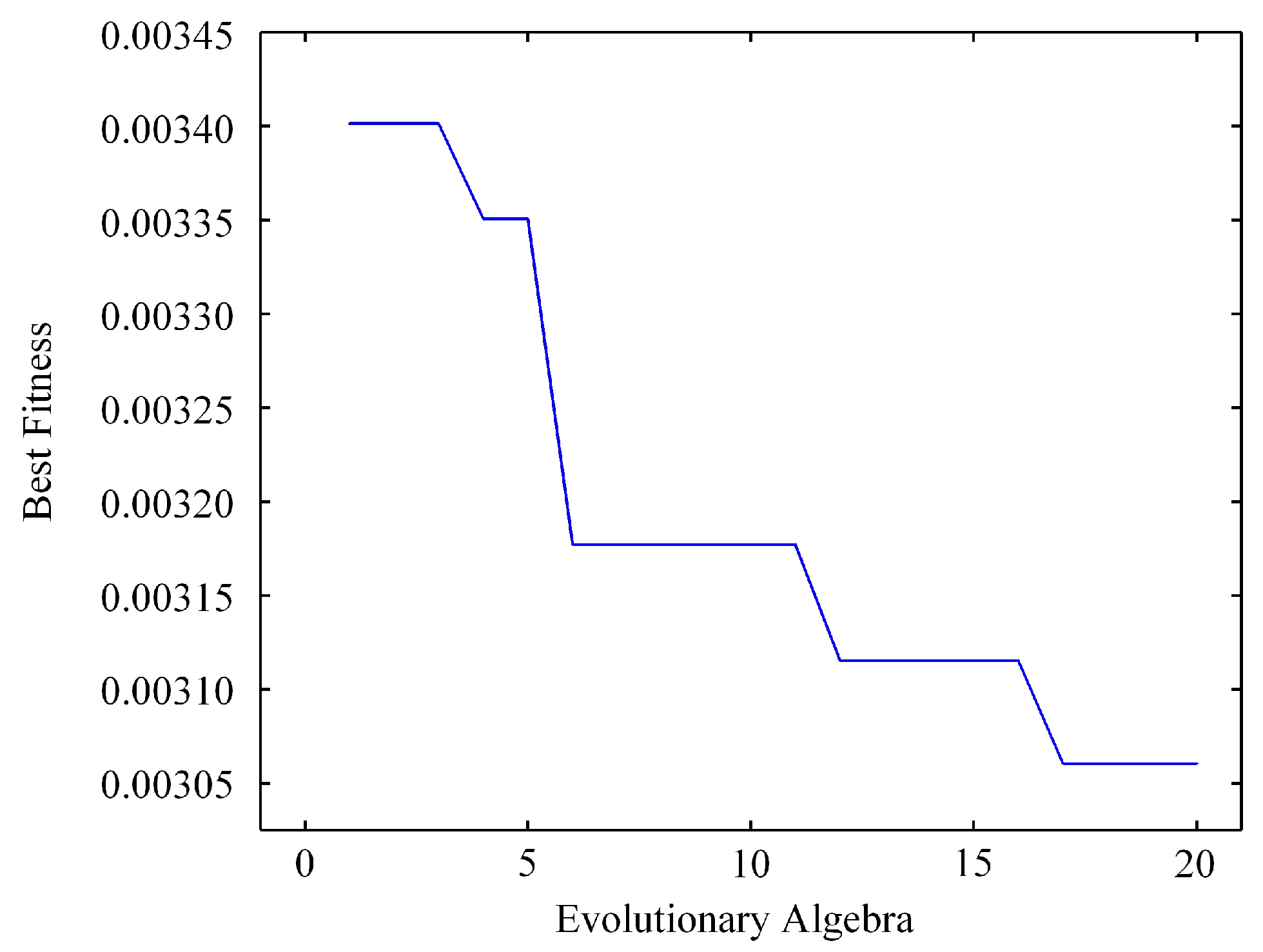
As shown in Figure 8, the validation fitness decreases as the population evolves and becomes stable at generation 17. The best mean squared error reaches 0.00307, which improves upon the baseline LSTM without GA that yields 0.00517 under the same protocol. The corresponding best chromosome is [2, 1, 40, 40, 0, 0, 0], indicating two LSTM layers and one dense layer with 40, 40, and 1 units, respectively. Under a fixed budget and the shared evaluation design, automatic architectural selection provides a better capacity-depth configuration within the constraints of early stopping and limited data. To keep the presentation focused, the detailed mechanics of the genetic operations are not repeated here; they follow the method descriptions already provided in this section. The results reported here should be interpreted as comparisons under the shared protocol described in Section 4.3, with the same windowing and normalization. Table 2 documents the baseline settings, the architectural search ranges of the GA-LSTM, and the GA budget, which ensures that configuration and capacity are traceable under the shared protocol. Figure 8 plots the best individual’s validation mean squared error across generations, shows an exploration then convergence pattern, and reports the final selected architecture together with its error.

Figure 8. Best fitness generation during GA search.

5.3. Result Analysis

Predictive performance is evaluated with root mean squared error (RMSE), mean absolute error (MAE), and mean absolute percentage error (MAPE) computed on normalized data, with definitions given by Equations (8)–(10). Results are reported for four input window lengths and for the comparison between the baseline LSTM and the GA-selected LSTM under the shared protocol described in Section 4.3.

$$RMSE=\sqrt{{\displaystyle \frac{{\sum }_{i=1}^N{(y_{truevalue}-y_{predictivevalue})}^2}{N}}}$$

(8)

$$MAE={\displaystyle \frac{1}{N}}\sum _{i=1}^N\left|y_{truevalue}-y_{predictivevalue}\right|$$

(9)

$$MAPE={\displaystyle \frac{1}{N}}\sum _{i=1}^N\left|{\displaystyle \frac{y_{truevalue}-y_{predictivevalue}}{y_{truevalue}}}\right|\times 100\%$$

(10)

All RMSE, MAE, and MAPE values reported in this subsection are single-run descriptive outcomes under the shared protocol (identical preprocessing, cycle-aligned inputs, train-set normalization, and device-stratified train/validation/test splits; selection uses validation loss on the same split; the test set is reserved for final reporting). The improvements ($\Delta$RMSE = 0.073; $\Delta$MAPE = 0.726%) should therefore be interpreted as point estimates subject to sampling variability. Statistical testing and confidence intervals are pre-specified in Methods and can be executed without changing the present setup.

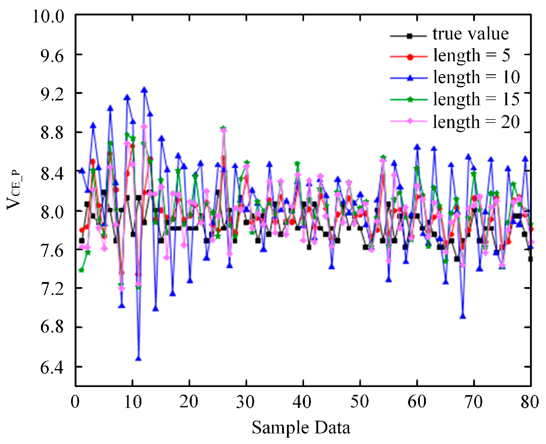
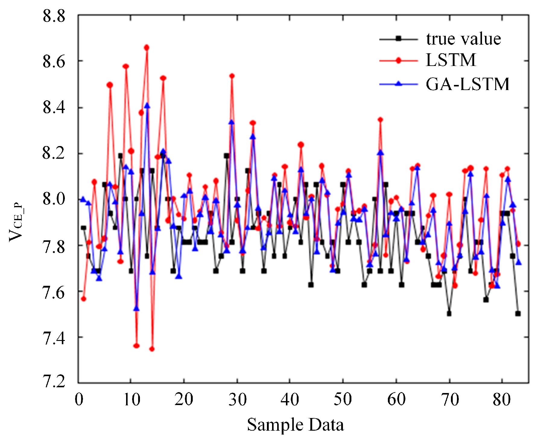
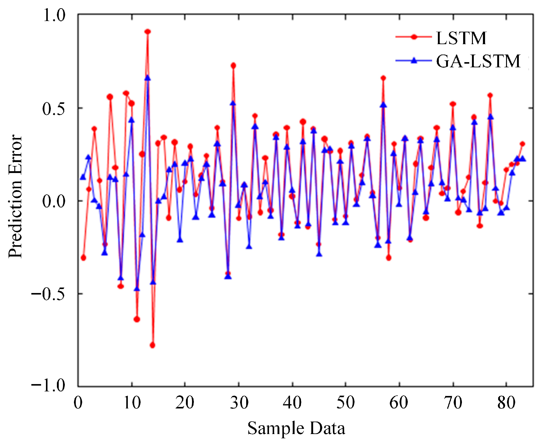
The window study indicates that short, event-centered inputs are most effective on this dataset. Table 5 and Figure 9 suggest that a five-step window yields the lowest errors (RMSE 0.319, MAE 0.253, MAPE 3.23%). At the same time, the ten-step setting reaches RMSE 0.596, consistent with noise accumulation and fewer effective sequences under longer histories. These observations support aligning the input length with the characteristic timescale of the degradation indicator so that local transients near the turn-off event are captured without excess variance. Under the same protocol, the GA-selected LSTM improves over the baseline configuration. Table 6, together with Figure 10 and Figure 11, shows that the GA-selected architecture reduces errors relative to the baseline LSTM (RMSE from 0.319 to 0.246; MAE from 0.253 to 0.196; MAPE from 3.233% to 2.507%), with the most significant gains at the beginning of the trajectory and a tighter per-cycle absolute-error profile. The curves in Figure 10 and Figure 11 correspond to baseline actual value (black), LSTM (red), and GA-LSTM (blue); the early-segment ordering described in the text can be cross-checked against the quantitative rankings in Table 6, so interpretation does not rely on color. Runtime and capacity are summarized in Table 7 under a shared environment and a fixed budget so that comparisons are reproducible. The table reports single-run wall-clock training time and memory usage. Times exclude data loading and plotting. GA search time is reported separately where applicable. These values are intended for descriptive comparison under the stated settings.

Table 5. Prediction performance evaluation of models with different lengths of sample data.

Input Length	RMSE	MAE	MAPE/%
5	0.319	0.253	3.233
10	0.596	0.486	6.204
15	0.417	0.343	4.387
20	0.405	0.335	4.277

Figure 9. Effect of input window length on forecasting. Axes show physical units; values are normalized where noted.

Table 6. Prediction performance evaluation of LSTM and GA-LSTM ¹.

Model	RMSE	MAE	MAPE/%
LSTM	0.319	0.253	3.233
GA-LSTM	0.246	0.196	2.507

¹ Figure 10 and Figure 11 provide visual context for these metrics; curve identification follows the color–model mapping stated in the figure captions, ensuring readability in grayscale.

Figure 10. Forecast trajectory of $V_{CE,p}$ (V) vs. cycle index (cycles) under the shared protocol. Axes show physical units; values are normalized where noted.

Figure 11. Per-cycle absolute error $V_{CE,p}$ (V) vs. cycle index (cycles) under the shared protocol. Axes show physical units; values are normalized where noted.

Table 7. The final parameter configuration of the optimized model is as follows.

Parameter	Optimal Configuration
LSTM Layers	2
Dense Layers	1
Neurons in LSTM Layers	40,40
Neurons in Dense Layer	1

Taken together, the results indicate that a five-step, cycle-aligned input gives the most favorable trade-off for this dataset, and that automatic architectural selection yields consistent descriptive gains under the shared protocol. The conclusions are specific to the single-indicator setting used here. The multivariate extension described in Section 3.2 can be evaluated under the same validation-based, fixed-budget procedure in future work.

For Table 6, metrics are single-run descriptive values obtained under the shared protocol. Variance across random seeds and 95% confidence intervals are not included in this revision. Still, they are pre-specified in Methods and can be reported without altering the data interface, splits, or selection rule. Reported times elsewhere refer to training in a fixed environment; per-sequence inference follows the configuration-dependent cost in Section 4.2 and is much smaller in wall-clock time because a short window is processed once per cycle after event-centered buffering. This distinction avoids conflating training cost with online monitoring cost.

5.4. Performance Comparison with Other Models

Under the shared preprocessing, device-stratified splits, and event-aligned inputs described in Section 5.3, GA-LSTM is compared with a baseline LSTM, CNN-LSTM, ARIMA, SVR, and EMD-LSTM. CNN-LSTM is known to couple spatial extraction with temporal modeling and has shown strong accuracy in multi-sensor fusion tasks [18]. ARIMA and SVR are representative statistical and machine-learning baselines in IGBT prognostics [10,12]. EMD-LSTM introduces signal decomposition before temporal learning and has reported competitive results on related datasets [19]. Within this context, GA-LSTM frames the problem as a compact sequence-forecasting task with automatic architectural selection, keeping the evaluation budget and protocol identical to all baselines. Recent IGBT studies with transformer-style models using multiscale attention have also reported competitive accuracy on NASA aging data; this line of work is complementary to our short, cycle-aligned formulation and can be evaluated under the same shared protocol.

Table 8 summarizes accuracy and runtime. GA-LSTM attains RMSE 0.246, MAE 0.196, and MAPE 2.507 percent, improving upon the baseline LSTM (0.319, 0.253, 3.233 percent). Relative to CNN-LSTM, which performs well on multivariate inputs [18], GA-LSTM achieves lower error on this single-indicator setting and trains faster under the fixed budget reported in the table. Statistical models show higher errors on this dataset: ARIMA reports RMSE 0.412 and MAPE 5.800 percent [12], and SVR reports RMSE 0.381 and MAPE 4.900 percent [10]. EMD-LSTM reaches RMSE 0.298 and MAPE 3.650 percent on similar IGBT data [19]; GA-LSTM outperforms it while avoiding extra decomposition steps. These comparisons support the conclusion from Section 5.3 that short, cycle-aligned inputs combined with automatic architectural selection offer a favorable depth-capacity match for early-stage changes.

Table 8. Performance and runtime under a shared protocol and a fixed environment ².

Parameter	GA-LSTM	LSTM	CNN-LSTM	ARIMA	SVR	EMD-LSTM
RMSE	0.246	0.319	0.287	0.412	0.381	0.298
MAE	0.196	0.253	0.221	0.327	0.301	0.238
MAPE/%	2.507	3.233	3.012	5.8000	4.9000	3.650
Training Time (s)	400	2000	600	<1	120	800
Memory Usage (MB)	45	30	80	-3	-	-
Input Length (Points)	5	5	5	-	-	-

² All models are evaluated under the shared protocol: identical preprocessing, event-centered cycle-aligned input windows, device-stratified train/validation/test splits, train-set–based normalization, and validation-based selection on the same split; the test set is used only for final reporting ³ - indicates not recorded.

Figure 10 and Figure 11 provide complementary evidence under the same protocol. Forecast trajectories show closer tracking to the ground truth for GA-LSTM than for the baseline LSTM and CNN-LSTM at the beginning of the sequence, where early-warning relevance is highest. The per-cycle absolute-error curves are consistently tighter for GA-LSTM. In contrast, competing models show larger deviations in mid-trajectory segments characterized by nonstationary fluctuations, which is consistent with the window-length study in Section 5.3. Together with Table 8, these figures indicate that GA-LSTM improves descriptive performance without increasing training cost in this setting.

Runtime and memory comparisons are reported under a fixed environment and a single-run budget; the corresponding assumptions are specified in the caption and table note of Table 8.

5.5. Future Research Directions

Building on the present results, physics-guided extensions will be explored under the same fixed-budget protocol. In line with recent PIML literature in PHM and condition monitoring, we will incorporate simple electro-thermal checks and consistency terms in the selection objective without changing the data interface. Examples include discouraging unrealistic ringing during turn-off and enforcing basic trend consistency between the on-state voltage and a thermal proxy. These additions keep the workflow reproducible and aim to improve robustness when operating conditions shift.

First, multivariate degradation indicators will be incorporated into the same cycle-aligned pipeline. In addition to the primary turn-off overvoltage, candidate inputs include the $V_{CE,on}$, the gate-to-emitter threshold voltage when it is measurable in practice, and a thermal-resistance proxy derived from transient thermal response. These quantities reflect complementary mechanisms in bond-wire and solder-layer degradation and are already observable in the waveforms used in Figure 4 and Figure 5. A multi-input sequence model, selected under the same fixed-budget procedure, can learn indicator weighting that is sensitive to the early trajectory, as illustrated in Figure 10 and Figure 11, which show the most significant practical benefit. The protocol for preprocessing, normalization, and device-stratified splits will remain unchanged so that comparisons stay reproducible.

Second, a hybrid physics-informed route will be explored to improve generalization. Simple electro-thermal constraints and consistency checks can be embedded in the fitness used for model selection without altering the data interface. Examples include penalties on unphysical oscillations during turn-off, temperature-trend consistency between the on-state voltage and the thermal proxy, and guardrails derived from basic energy considerations. Where appropriate, physics-based simulations can be used to generate boundary-case scenarios to probe the model outside the NASA PCoE operating band while keeping the evaluation on measured data. This direction addresses the domain-shift limitations noted in Section 5.3 and keeps the link between the mechanism and the observable explicit.

Third, adaptive configuration under deployment will be considered. While the present genetic algorithm operates with fixed rates and a fixed budget, future work can adjust mutation and selection pressure based on validation feedback or simple reinforcement signals that reflect changes in the operating regime. The objective is to retain a compact architecture on stable regimes and to permit controlled exploration when load profiles or cooling conditions shift. Any adaptation will be evaluated under a locked test set and with the same reporting of wall-clock cost and capacity used in Section 5.4.

Figures and tables motivate these directions without requiring new metrics. Figure 4 and Figure 5 demonstrate that the chosen indicators are both measurable and informative regarding the turn-off event, thereby supporting multivariate inputs that capture both the electro-thermal state and the evolution of conduction paths. Figure 10 and Figure 11 show that most gains appear at the beginning of the trajectory, which suggests early-segment weighting or constraints focused on that region. Future evaluations will keep the definitions in Equations already provided, retain the single-protocol design, and add multi-run statistics when additional data are available.

As shown in Figure 12, a physics-guided variant can be obtained by augmenting the forecasting loss with lightweight electro-thermal consistency terms while keeping the same inputs and splits. Let $L_p$ denote the data-fit term (e.g., RMSE on the indicator window), and let ${\lambda }_1,{\lambda }_2,{\lambda }_3$ $\ge 0$ be user-set weights. We define

$$L_{to}=L_p+{\lambda }_1{L}_t+{\lambda }_2{L}_r+{{\lambda }_{3}L}_{ph}$$

(11)

where the term $L_t$ encourages temperature-consistent behavior of the conduction-phase voltage, for example by penalizing violations of an expected trend between the $V_{CE,on}$ and a junction-temperature proxy estimated from the same window. The term $L_r$ damps unphysical high-frequency ringing in the predicted turn-off transient, consistent with passive parasitics measured on the device. The term $L_{ph}$ softly enforces bounds that reflect safe operating limits, such as reasonable ranges for $\mathrm{d}V/\mathrm{d}t$ during turn-off or for the $V_{CE,p}$. Because these terms act on the same cycle-aligned windows and measured indicators used throughout the paper, they do not alter the data interface, the preprocessing, or the train/validation/test splits; they guide the forecaster toward electro-thermally plausible trajectories.

Figure 12. Clean implementation sketch for a physics-informed extension. Inputs are short, event-centered, cycle-aligned windows of measurable indicators.

6. Conclusions

This study frames IGBT health prediction as a device-centric short-sequence task and reports a sequence model that uses measurable, event-centered indicators. The practical implication is that routine monitoring can focus on the turn-off instant and a small, cycle-aligned window, which reduces data volume while preserving the information most relevant to early degradation. In maintenance planning, the recommended use is to track the peak turn-off overvoltage as the primary indicator and the $V_{CE,on}$ as a complementary indicator of conduction path and temperature.

For predictive maintenance scheduling, forecasts can be used to trigger actions based on anticipated threshold crossings of the primary indicator. When the predicted trajectory approaches a predefined health limit within the planning horizon, operators can schedule inspection, tighten thermal management, or temporarily derate the converter. When the forecast uncertainty widens or the residuals show a sustained upward drift at the beginning of the trajectory, a preventive check of bond-wire and solder-layer interfaces is advised. These rules translate the descriptive accuracy gains into earlier interventions without adding training cost under the reported environment. For early failure prevention, the sequence model supports condition-aware thresholds. Event-centered inputs emphasize the first portion of the trajectory, where small changes are most informative for impending faults. Maintenance teams can assign higher weight to early-segment deviations and use conservative trigger margins when the operating regime changes or when ambient cooling is reduced. This approach allows conservative protection without frequent false alarms. For deployment, three requirements are recommended. First, acquire cycle-aligned records with sufficient sampling density around the turn-off to ensure consistent extraction of indicators. Second, ensure that preprocessing and normalization remain stable across devices and time, and utilize training-set statistics when applying the model in production. Third, use a simple calibration when the operating band shifts, and validate on a held-out subset before rolling out changes. These steps keep the workflow reproducible and compatible with existing data pipelines. The thermo-mechanical chain from solder-layer voiding to junction-temperature rise and altered turn-off transients [27], together with the demonstrated sensitivity of the thermal field to cooling-channel design [28], supports event-centered acquisition around turn-off and clarifies why the stability of $V_{CE\_p}$ and $V_{CE\_on}$ in field monitoring depends on local thermal management. The same event-centered acquisition and short windows enable a physics-informed variant by adding minor electro-thermal consistency penalties to the forecasting loss, which can improve plausibility without changing the data interface or deployment workflow.

Real-time use relies on event-centered buffering around turn-off, indicator computation, and a single forward pass on a short window. With low-dimensional inputs and short windows, inference cost follows the configuration-dependent form. It is typically dominated by data capture rather than the model itself, making per-cycle evaluation feasible on microcontroller- or SoC-class CPUs. This guidance leaves the shared protocol unchanged and clarifies how the model can be used in practice.

The reported results are single-run and descriptive under a fixed budget. To support fleet-level decisions, future work will add multi-run statistics and extend the inputs to multivariate indicators within the same protocol. A lightweight physics-informed selection objective will also be explored to discourage unphysical oscillations and to improve stability under condition shifts. These extensions keep the evaluation consistent while improving robustness for predictive maintenance in electric vehicles, renewable-energy conversion, and industrial drives.

References

1. Baliga, B.J. Trends in power semiconductor devices. IEEE Trans. Electron Devices 1996, 43, 1717–1731. [Google Scholar] [CrossRef]
2. Li, Q.; Zhang, F.; Chen, Y.; Fu, T.; Zheng, Z. A junction temperature model based on heat flow distribution in an IGBT module with solder layer voids. Heliyon 2024, 10, e33625. [Google Scholar] [CrossRef] [PubMed]
3. Ahsan, M.; Hon, S.T.; Batunlu, C. Reliability assessment of IGBT through modelling and experimental testing. IEEE Access 2020, 8, 39561–39573. [Google Scholar] [CrossRef]
4. Li, J.; Wang, D.; Deng, L.; Cui, Z.; Lyu, C.; Wang, L.; Pecht, M. Aging modes analysis and physical parameter identification based on a simplified electrochemical model for lithium-ion batteries. J. Energy Storage 2020, 31, 101538. [Google Scholar] [CrossRef]
5. Wang, D.; Yang, F.; Zhao, Y.; Tsui, K.-L. Battery remaining useful life prediction at different discharge rates. Microelectron. Reliab. 2017, 78, 212–219. [Google Scholar] [CrossRef]
6. Thebaud, J.M.; Woirgard, E.; Zardini, C. Strategy for designing accelerated aging tests to evaluate IGBT power modules lifetime in real operation mode. IEEE Trans. Compon. Packag. Technol. 2003, 26, 429–438. [Google Scholar] [CrossRef]
7. Zio, E.; Peloni, G. Particle filtering prognostic estimation of the remaining useful life of nonlinear components. Reliab. Eng. Syst. Saf. 2011, 96, 403–409. [Google Scholar] [CrossRef]
8. Kova, I.F.; Drofenik, U.; Kolar, J.W. New physical model for lifetime estimation of power modules. In Proceedings of the 2010 International Power Electronics Conference—ECCE ASIA, Sapporo, Japan, 21–24 June 2010; pp. 2106–2114. [Google Scholar]
9. Ahsan, M.; Stoyanov, S.; Bailey, C. Data driven prognostics for predicting remaining useful life of IGBT. In Proceedings of the 2016 39th International Spring Seminar on Electronics Technology (ISSE), Pilsen, Czech Republic, 18–22 May 2016; pp. 273–278. [Google Scholar]
10. Ismail, A.; Saidi, L.; Sayadi, M.; Benbouzid, M. A new data-driven approach for power IGBT remaining useful life estimation based on feature reduction technique and neural network. Electronics 2020, 9, 1571. [Google Scholar] [CrossRef]
11. Li, W.; Wang, B.; Liu, J.; Zhang, G.; Wang, J. IGBT aging monitoring and remaining lifetime prediction based on long shortterm memory (LSTM) networks. Microelectron. Reliab. 2020, 114, 113902. [Google Scholar] [CrossRef]
12. Xie, F.; Tang, X.; Shen, H.; Luo, Y. A GRU-Based Method of IGBT Module Degradation Prediction Under Changing Working Conditions. In Proceedings of the 2022 Global Reliability and Prognostics and Health Management (PHM-Yantai), Yantai, China, 28–30 October 2022; pp. 1–6. [Google Scholar]
13. Hochreiter, S.; Schmidhuber, J. Long short-term memory. Neural Comput. 1997, 9, 1735–1780. [Google Scholar] [CrossRef]
14. Weikun, D.; Nguyen, K.T.; Medjaher, K.; Christian, G.; Morio, J. Physics-informed machine learning in prognostics and health management: State of the art and challenges. Appl. Math. Model. 2023, 124, 325–352. [Google Scholar] [CrossRef]
15. Wu, Y.; Sicard, B.; Gadsden, S.A. Physics-informed machine learning: A comprehensive review on applications in anomaly detection and condition monitoring. Expert Syst. Appl. 2024, 255, 124678. [Google Scholar] [CrossRef]
16. Lu, Z.; Guo, C.; Liu, M.; Shi, R. Remaining useful lifetime estimation for discrete power electronic devices using physics-informed neural network. Sci. Rep. 2023, 13, 10167. [Google Scholar] [CrossRef]
17. He, S.; Yu, M.; Chen, Y.; Zhou, Z.; Yu, L.; Zhang, C.; Ni, Y. Prediction of IGBT Gate Oxide Layer’s Performance Degradation Based on MultiScaleFormer Network. Micromachines 2024, 15, 985. [Google Scholar] [CrossRef]
18. Kim, T.Y.; Cho, S.B. Predicting Residential Energy Consumption Using CNN-LSTM Neural Networks. Energy 2019, 182, 72–81. [Google Scholar] [CrossRef]
19. Borgo, M.D.; Tehrani, M.G.; Elliott, S.J. Elliott Identification and Analysis of Nonlinear Dynamics of Inertial Actuators. Mech. Syst. Signal Process. 2019, 115, 338–360. [Google Scholar] [CrossRef]
20. Zhang, Z.; Qin, R.; Li, G.; Du, Z.; Li, Z.; Lin, Y.; He, W. Deep Learning-Based Monitoring of Surface Residual Stress and Efficient Sensing of AE for Laser Shock Peening. J. Mater. Process. Technol. 2022, 303, 117515. [Google Scholar] [CrossRef]
21. Mukherjee, S.; Wang, S.; Wallace, A. Interacting, Vehicle Trajectory Prediction with Convolutional Recurrent Neural Networks. In Proceedings of the 2020 IEEE International Conference on Robotics and Automation (ICRA), Paris, France, 31 May–31 August 2020; pp. 4336–4342. [Google Scholar]
22. El-Kenawy, E.-S.M.; Khodadadi, N.; Mirjalili, S.; Abdelhamid, A.A.; Eid, M.M.; Ibrahim, A. Greylag Goose Optimization: Nature-inspired optimization algorithm. Expert Syst. Appl. 2024, 238, 122147. [Google Scholar] [CrossRef]
23. Ord’o, F.J.; Roggen, D. Deep convolutional and lstm recurrent neural networks for multimodal wearable activity recognition. Sensors 2016, 16, 115. [Google Scholar] [CrossRef] [PubMed]
24. Ji, B.; Pickert, V.; Cao, W.; Zahawi, B. In situ diagnostics and prognostics of wire bonding faults in IGBT modules for electric vehicle drives. IEEE Trans. Power Electron. 2013, 28, 5568–5577. [Google Scholar] [CrossRef]
25. Du, X.; Zhang, J.; Li, G.; Tai, H.M.; Sun, P.; Zhou, L. Lifetime estimation for IGBT modules in wind turbine power converter system considering ambient temperature. Microelectron. Reliab. 2016, 65, 69–78. [Google Scholar] [CrossRef]
26. Wang, M.Y.; Lu, G.Q.; Mei, Y.H.; Li, X.; Wang, L.; Chen, G. Electrical method to measure the transient thermal impedance of insulated gate bipolar transistor module. IET Power Electron. 2015, 8, 1009–1016. [Google Scholar] [CrossRef]
27. Xu, P.; Liu, P.; Yan, L.; Zhang, Z. Effect of Solder Layer Void Damage on the Temperature of IGBT Modules. Micromachines 2023, 14, 1344. [Google Scholar] [CrossRef] [PubMed]
28. Tan, L.; Liu, P.; She, C.; Xu, P.; Yan, L.; Quan, H. Heat dissipation characteristics of IGBT module based on flow-solid coupling. Micromachines 2022, 13, 554. [Google Scholar] [CrossRef]
29. Celaya, J.; Wysocki, P.; Goebel, K. IGBT Accelerated Aging Data Set. In NASA Prognostics Data Repository; NASA Ames Research Center: Moffett Field, CA, USA, 2009; Archive: “8.+IGBT+Accelerated+Aging.zip”. Available online: https://www.nasa.gov/intelligent-systems-division/discovery-and-systems-health/pcoe/pcoe-data-set-repository/ (accessed on 1 April 2023).
Disclaimer/Publisher’s Note: The statements, opinions and data contained in all publications are solely those of the individual author(s) and contributor(s) and not of MDPI and/or the editor(s). MDPI and/or the editor(s) disclaim responsibility for any injury to people or property resulting from any ideas, methods, instructions or products referred to in the content.
Article Metrics
Citations
Article Access Statistics
Article metric data becomes available approximately 24 hours after publication online.