Short-Term Electrical Load Forecasting Based on XGBoost Model

Abstract

Forecasting electricity consumption is one of the most important scientific and practical tasks in the field of electric power engineering. The forecast accuracy directly impacts the operational efficiency of the entire power system and the performance of electricity markets. This paper proposes algorithms for source data preprocessing and tuning XGBoost models to obtain the most accurate forecast profiles. The initial data included hourly electricity consumption volumes and meteorological conditions in the power system of the Republic of Tatarstan for the period from 2013 to 2025. The novelty of the study lies in defining and justifying the optimal model training period and developing a new evaluation metric for assessing model efficiency—financial losses in Balancing Energy Market operations. It was shown that the optimal depth of the training dataset is 10 years. It was also demonstrated that the use of traditional metrics (MAE, MAPE, MSE, etc.) as loss functions during training does not always yield the most effective model for market conditions. The MAPE, MAE, and financial loss values for the most accurate model, evaluated on validation data from the first 5 months of 2025, were 1.411%, 38.487 MWh, and 16,726,062 RUR, respectively. Meanwhile, the metrics for the most commercially effective model were 1.464%, 39.912 MWh, and 15,961,596 RUR, respectively.

1. Introduction

The modern wholesale electricity market (WEM) is a dynamic and complex system where electricity is primarily traded through competitive bidding processes [1]. The WEM serves as a trading platform that integrates generation companies, grid operators, distribution dispatch centers, and energy supply companies.

The function of this market is to balance electricity supply and demand through market mechanisms, thereby synchronizing power generation and consumption processes [1,2].

The WEM includes three trading sectors: the Day-Ahead Market (DAM), the Balancing Energy Market (BEM), and the regulated contracts sector (Figure 1).

ESCs, as key consumers, must submit to the DAM hourly electricity purchase bids for the next operating day, with daily submissions required. The Trading System Administrator (TSA), also known as the Market Operator (MO), processes the collected bids and forwards them to the System Operator (SO). The SO generates a dispatch schedule that determines the power output allocation for generating units. Deviations between actual consumption and DAM forecast bids are settled by consumers at higher BEM tariffs.

Sometimes such deviations may exceed permissible limits (3–5%) set by the regulator. In such cases, all market participants bear losses: large consumers, due to significant BEM overpayments; the SO, from disrupted grid operating conditions; grid companies facing line overloads and increased losses in some sections while other network equipment remains underutilized; and energy suppliers experiencing worsened performance metrics as generators deviate from pre-calculated optimal load zones. Furthermore, generation companies incur imbalance charges due to deviations between their actual natural gas consumption and nominated schedules with regional gas suppliers, caused by power system balancing operations.

Such deviations are most commonly associated with the growing complexity of power systems, caused by the rapid spread of distributed energy resources (including renewables [1,4,5,6,7]); the proliferation of electrified transport [5,7,8]; consumer response to demand [6,8,9,10]; and climate change effects [11,12].

Even a 1% increase in the accuracy of consumer demand forecasts can lead to significant cost reductions for all market participants. Furthermore, an increase in accuracy improves the energy efficiency of power and heat generation equipment, enhances power system stability, and strengthens supply reliability for consumers. Abbas M. et al. [2], Gong J. et al. [13], and Yang D. et al. [14] highlighted that even a 1% forecasting inaccuracy may cost power utilities millions of US dollars.

Thus, the field of this study—short-term load forecasting (STLF)—is of critical importance to all participants of the WEM [5,6,8,9].

Short-term load forecasting (STLF) operates on a 24 h timeframe. This differs from mid- and long-term forecasting (MTLF/LTLF), which use monthly and annual horizons, respectively [12]. Consequently, STLF demonstrates higher sensitivity to dynamic external factors, such as temperature fluctuations or electricity price variations [9,12]. The relationship between electricity demand and external factors frequently exhibits strong nonlinearity, making STLF an exceptionally challenging task [2,9].

Currently, a variety of forecasting methods are used to solve such a complex and important scientific problem as STLF. Forecasting methods are conventionally divided into four main groups: 1) traditional statistical approaches (ARIMA, SARIMA, GARCH, exponential smoothing); 2) machine learning (ML) methods (SVM, RF, GB, XGBoost, KNN); 3) deep learning (DL) methods for time-series analysis (Transformers, LSTM, CNN, MLP); and 4) hybrid approaches [8,12,15].

Classical statistical models like ARIMA (Autoregressive Integrated Moving Average) effectively capture the cyclical patterns of energy consumption caused by seasonal factors [6]. However, due to their linear structure, they cannot account for exogenous variables with complex nonlinear dependencies [4,15]. ML algorithms do not have this problem. They can process both categorical features (e.g., day of week, day type: weekday, weekend, holiday, pre-holiday) and numerical features (temperature, electricity price) [8,15]. However, these algorithms are susceptible to overfitting if their hyperparameters are not properly tuned [4].

More advanced and specialized ML methods for STLF tasks include DL approaches for time-series analysis. These approaches are particularly effective at modeling long-term temporal dependencies and complex nonlinear relationships, offering robust generalization performance [5,8]. However, these methods suffer from limited interpretability [4] and high computational demands [6,8], and sometimes do not show the highest efficiency. Additionally, multiple studies highlight their vulnerability to vanishing gradient problems with very long sequences [2,8,10,16].

The recent scientific literature shows growing interest in hybrid models. By combining the strengths of multiple algorithms, these models often outperform standalone ML and DL approaches [4]. However, they come with notable drawbacks: higher design and implementation complexity, greater expertise requirements for development and maintenance, increased computational demands compared to DL models, poor interpretability, and limited scalability to other power systems.

The aim of this study was to develop a simple, fast, and interpretable ML model with MAPE < 1.5%, along with a validation mechanism that closely replicates real-world conditions.

The study achieved the following key results:

• The nomenclature, volume, and availability of data for model development were evaluated, and a data preprocessing pipeline was developed;
• Four STLF XGBoost models with a simple tuning mechanism and high interpretability were developed;
• A method for preliminary hyperparameter tuning was proposed, which significantly increased the computational speed from ~30 s/it to ~2 s/it;
• New loss functions for model training and testing were developed, accounting for electricity market pricing specifics;
• The optimal training dataset size was determined for models that consider (6 years) and do not consider (10 years) the Balancing Market Index (BMI);
• A model with commercially viable error was developed: MAPE = 1.411%, MAE = 38.487 MWh.

Accordingly, this paper has the following structure. Section 2 analyzes recent experience (2024–2025) in the application of ML to the STLF problem, assesses the current state of research in this field, and briefly outlines the most common models and evaluation metrics. Section 3 introduces the source and structure of the input data, provides a concise explanation of the XGBoost (eXtreme Gradient Boosting) regressor algorithm, details the hyperparameter tuning mechanism, describes the proposed loss function used as a supplement to traditional MAE and MAPE metrics, examines the suggested validation approach for ML models, and lists the software and hardware used. Section 4 presents a feature importance analysis, identifies the most significant factors in the context of STLF, determines and justifies optimal training periods (test set size) for the models, and compares and evaluates the accuracy and efficiency of the resulting ML models. Concluding remarks are introduced in Section 5.

2. The Current State of the Research Area

Table 1. Summary of ML models for load forecasting.

Reference	Publ.	Best Model	Data Size	Train/Test/Validation Set	Count Features	Error Metrics
Abbas M. et al. [2]	2025	AdaBoost-LGB-MLP-KAN	5 years	4:1:0	21	MAPE = 2.05%, RMSE = 353.52 MW, MAE = 289.96 MW
Zhao Q. et al. [5]	2025	TPE-XGB-CS-BiLSTM	3 years	1:1:1	286	MAE = 27.77 MW, RMSE = 40.45 MW MAPE = 2.98%, R2 = 94.06
Karamolegkos S., Koulouriotis D.E. [6]	2025	FARIMA	10 years	51:1:0	3	MAPE = 7.96%, RMSE = 813.98, MSE = 662,556.46
Liu M. et al. [7]	2025	iMICN	5 years	8:1:1	7	MAPE = 0.41%, MAE = 62.12 MW, RMSE = 202.23 MW
Zhao J. et al. [8]	2024	LASTGCN	16 months	7:2:1	31	MAE = 0.0246 MWh, RMSE = 0.0455, R2 = 0.7991
Wang B. et al. [9]	2025	CEEMDAN-CNN-BiLSTM	25 days	25:1:0	5	RMSE = 154.2101 MW, R2 = 0.98333, MAE = 117.4744 MW, MAPE = 1.396%
Xu F. et al. [10]	2024	VMD-Nyströmformer-BiTCN	1 year	50:3:0	1	MAE = 8.35, SAE = 0.042
Ning Z. et al. [11]	2025	TKNFD-Transformer	15 years	12:3:0	38–92	MAPE ≈ 1.4%
Ullah K. et al. [12]	2024	CNN-LSTM	53 months	34:15:5	10	RMSE = 951.94, MAE = 656.35, MAPE = 4.72%
Gong J. et al. [13]	2025	TCN-LSTM-LGB	5 years	6:2:2	7	MAPE = 0.519%, MAE = 46.1 MW, RMSE = 62.3 MW
Yang D. et al. [14]	2023	ICEEMDAN-PE-BP	4 months	60:20:20	1	MAE = 175.595, RMSE = 223.525, MAPE = 0.78
Osgonbaatar T. et al. [15]	2023	XGB	3 years	70:30:0	16	MAE = 10.76 MW, MAPE = 1.25%
Chen J. et al. [16]	2024	MVMO-LSTM	1 year	70:30:0	4	RMSE = 0.1564, MAE = 0.1215, R2 = 0.9918
Luo H. et al. [17]	2025	2D CNN-GASF-GADF-RP	12 years	80:20:0	4	MAE = 234, RMSE = 339, MAPE = 1.55%, R2 = 0.983
Zhang L., Jánošík D. [18]	2024	XGB-AOA	1 year	7884:876:0	5	RMSE = 4227, MAPE = 0.05973 R2 = 0.92252
Timur O., Üstünel H.Y. [19]	2025	GB	3 years	80:20:0	15	R2 = 98.591, MAPE = 0.827%
Zhou B. et al. [20]	2024	FA-BiGRU-A	2 years	20:2:2	8	MAE = 0.581 MW, RMSE = 0.871 MW MAPE = 2.037%
Brahim S.B. et al. [21]	2025	Transformer-BiLSTM-DA	2 years	60:20:20	9	R2 = 0.038, RMSE = 0.0022, MAPE = 0.0176
Ghimire S. et al. [22]	2024	VMD-CABiLSTM-ANN-EC	10 years	50:50:0	1	RMSE = 0.187 MW, MAE = 0.137 MW RMAE = 1.145%, RRMSE = 3.624%
Chen C. et al. [23]	2024	ARM	1 months	2880:96:0	13	RMSE = 256.17 MW, MAPE = 1.982%, R2 = 0.989
Zhang M. et al. [24]	2023	ICEEMDAN-CNN-BiLSTM	1 month	70:20:10	11	MAPE = 1.85, RMSE = 0.407 kW
Pavlatos C. et al. [25]	2023	BiLSTM	746 days	25:6:1	1	RMSE = 0.022, MAE = 0.122
Pinto T. et al. [26]	2021	AdaBoost	10 days	10:1:0	15	MAPE = 5.34%
Sheng Z. et al. [27]	2023	DRN-LSTM-SEN	4324 days	32:12:0	1	MAPE = 1.56%
Han X. et al. [28]	2023	IWOA-KELM	7 days	6:1:0	2	MAPE = 1.25%, RMSE = 13.62
Stamatellos G. et al. [29]	2023	FF ANN	6 years	5:1:0	7	MAPE = 3.66%, RMSE = 0.049
Shahare K. et al. [30]	2023	CNN-LSTM	2 years	70:30:0	6	MAE = 0.043, RMSE = 0.064, R2 = 95.05%
Wan A. et al. [31]	2023	CNN-LSTM-A	1 year	4:1:0	9	MAPE = 2.85%, RMSE = 0.6175
Aguilar Madrid E., Antonio N. [32]	2021	XGB	65 months	51:14:0	13	MAPE = 3.74%, RMSE = 55.6, PEAK = 2.93, VALLEY = 3.04, ENERGY = 1.75
Hasanat S.M. et al. [33]	2024	1-D CNN-GRU	–	–	10	MAE = 686.32, MAPE = 3.24%, RMSE = 486.17
Sekhar C., Dahiya R. [34]	2023	1-D GWO-CNN-BiLSTM	50 months	90:10:0	4	MAE = 0.212, MSE = 0.119, MAPE = 0.0699, RMSE = 0.265
Ran P. et al. [35]	2023	CEEMDAN-SE-Transformer	1 year	80:20:0	3	MAPE = 4.8%, RMSE = 1.26, MAE = 0.95, R2 = 0.8
Wei N. et al. [36]	2024	WM-DSSFA-LSTM-TL	6 years	4:1:1	6	MAE = 0.4, RMSE = 0.51, R2 = 0.41, MAPE = 15.66%, MARNE = 9.28%
Yamasaki M. et al. [37]	2024	XGB-EWT	5 years	130:15:0	175	RMSE = 1 931.8 MW, MAE = 1 564.9 MW, MAPE = 2.54%
Asiri M.M. et al. [38]	2024	CNN-BiLSTM-AE	31 days	30:1:0	1	MAPE = 0.059%
Tarmanini C. et al. [39]	2023	ANN	18 months	90:10:0	1	MSE = 174.4, MAPE = 1.8%
Dong J. et al. [40]	2025	BiGRU-ASAE	1 year	–	13	MAPE = 1.37%
Cavus M., Allahham A. [41]	2025	CNN-LSTM-A	1 year	–	3	MAE = 0.0485, RMSE = 0.0795, MAPE = 0.1156, R2 = 0.4867
Ali A. et al. [42]	2025	ADMGM	8 months	4656:240:0	128	MAPE = 15.21%, RMSE = 2.14
This study	2025	XGB	149 months	132:12:5	18	MAE = 38.487 MWh, MAPE = 1.411%

presents a summary of recent studies (2024–2025) on the development of ML-based power consumption forecasting models.

The performance and accuracy of STLF models are most commonly evaluated using the following metrics:

• The mean absolute error (MAE), as follows:

  $$\mathrm{MAE}={\displaystyle \frac{1}{n}}\cdot {\displaystyle \sum _{i=1}^n\left|A_i-P_i\right|}$$

  (1)
• The mean absolute percentage error (MAPE), as follows:

  $$\mathrm{MAPE}={\displaystyle \frac{1}{n}}\cdot {\displaystyle \sum _{i=1}^n\frac{\left|A_i-P_i\right|}{A_i}}$$

  (2)
• The mean squared error (MSE), as follows:

  $$\mathrm{MSE}={\displaystyle \frac{1}{n}}\cdot {\displaystyle \sum _{i=1}^n{\left(A_i-P_i\right)}^2}$$

  (3)
• The root mean square error (RMSE), as follows:

  $$\mathrm{RMSE}=\sqrt{{\displaystyle \frac{1}{n}}\cdot {\displaystyle \sum _{i=1}^n{\left(A_i-P_i\right)}^2}}$$

  (4)
• The coefficient of determination (R²), as follows:

  $$R^2=1-{\displaystyle \frac{{\displaystyle \sum _{i=1}^n{\left(A_i-P_i\right)}^2}}{{\displaystyle \sum _{i=1}^n{\left({\overline{A}}_i-P_i\right)}^2}}}$$

  (5)

  where A_i and P_i are the actual and predicted values, respectively; ${\overline{A}}_i$ is the sample average; and n is the validation sample size.

In the context of STLF model evaluation, MAPE is the most relevant and widespread metric used by researchers. This metric enables proper comparison of STLF model performance across power systems of varying scales—from small grids serving just a few households [21,26,34] to national-scale power systems [2,5,6,15,29]. However, the MAPE metric is not able to compare the commercial efficiency of two different models, and therefore does not always reflect the real state.

Recognizing this problem, some researchers have attempted to introduce their own metrics: IMB [5]; PIPC, PINAW, CWC, PIT and CRPSO [7]; RMAE and RRMSE [22], penalty [27]; PEAK, VALLEY and ENERGY [32]; and MARNE [36]. However, all of these penalty functions are aimed at a more detailed comparison of models’ predictive accuracy, rather than for assessing their commercial efficiency. Therefore, there is a clear need to develop evaluation metrics that incorporate the specifics of electricity market pricing mechanisms, since the model’s predictive accuracy does not always directly correlate with its commercial efficiency.

According to Table 1, hybrid models have been gaining significant popularity among researchers in recent years: in 25 out of 38 reviewed publications, authors propose their own unique hybrid models. The most effective models in terms of the MAPE metric (2) include the following: CEEMDAN-CNN-BiLSTM (1.3956%) [9]; TKNFD-Transformer (1.4%) [11]; TCN-LSTM-LGB (0.519%) [13]; 2D CNN-GASF-GADF-RP (1.55%) [17]; DRN-LSTM-SEN (1.56%) [27]; IWOA-KELM (1.25%) [28]; CNN-BiLSTM-AE (0.059%) [38]; and BiGRU-ASAE (1.37%) [40].

This variety of unique hybrid models, coupled with the lack of reproducible results when other researchers try to apply these models to their own datasets, demonstrates their inability to scale across power systems. Hybrid models are inherently optimized for their initial datasets, and consequently cannot be considered as universal solutions.

More scalable solutions include ML and DL models. According to Table 1, the most common DL models are LSTM, CNN, TCN, RNN, and their analogues. Zhao J. et al. [8] also came to similar conclusions in their study. At the same time, Table 1 reveals that standalone DL models do not show the best results.

Traditional ML models remain quite popular and, despite their simplicity and computational efficiency, demonstrate competitive performance. In 6 out of 38 reviewed publications, basic (MLR, SVM, etc.) and ensemble (RF, GB, XGB, AdaBoost, etc.) ML models outperformed hybrid and DL models. The most accurate models in terms of MAPE were XGBoost (1.25%) [15] and GB (0.829%) [19].

Thus, among the 38 publications analyzed, only 10 models demonstrate potential commercial viability (MAPE < 1.5%). These are predominantly hybrid models with poor interpretability, high computational complexity, and limited scalability. The problem is that most authors (e.g., [2,5,8,9,14,16,20,22,35,37]) focus on hyperparameter tuning and increasing model complexity instead of improving data preprocessing quality and robustness. It is widely recognized that data and features set the upper bound for ML model performance, while models and their algorithms merely approximate this limit [11]. Authors who move beyond conventional time-series analysis and incorporate spatial feature matrices into their models typically achieve superior results. As shown in Table 1, the mean number of input features across studies is 20, and the median is 7. Given the complexity and multifaceted nature of STLF tasks, this number of input features may prove insufficient.

The average data collection period used by authors for training, tuning, and testing their models is 44 months, with a median of 24 months (2 years). The maximum observed timeframe is 15 years [11], while the minimum is just 7 days [28]. It should be noted that empirical justification for selecting the model training period has only been performed in the study of Karamolegkos S. and Koulouriotis D.E. [6]. This aspect is critically important, as an insufficient amount of data can lead to model underfitting, resulting in the inability of the model to capture complex underlying patterns. Conversely, an excessive amount of data can lead to model overfitting due to the use of outdated and irrelevant information.

Among all 38 studies reviewed, only in 11 studies was model performance evaluated using a closed validation set. Consequently, just one model—TCN-LSTM-LGB [13]—demonstrated a commercially viable error level, with its reliability confirmed through blind validation testing.

The scientific novelty of this study consists of the following:

• First, systematic determination of the optimal data collection duration for STLF model training, supported by theoretical analysis;
• Development of a novel Financial Loss function to quantify operational costs in the BEM for specified periods;
• Development of a blind validation mechanism that replicates real-world conditions for rigorous STLF model testing.

3. Materials and Methods

3.1. Data Collection

The research data was provided by the largest ESC of the Republic of Tatarstan. This region is one of nine participants in the Unified Energy System (UES) of the Middle Volga region. Notably, the Republic of Tatarstan accounts for up to 40% of total energy consumption within this regional UES.

The dataset contains measured electricity load values from 1 January 2013 to 10 June 2025 with hourly resolution. To build a comprehensive model that reliably reflects the complex relationships between power consumption and exogenous factors, this dataset was expanded with weather and calendar features, as well as data from the SO.

According to the study by Osgonbaatar T. et al. [15], ambient air temperature has the most significant impact on electricity consumption at the regional power system level, while other meteorological indicators (humidity, cloud cover, wind speed/direction, etc.) show negligible effects. Therefore, only temperature data was added to the dataset from the source https://kazan.nuipogoda.ru/ (accessed on 10 June 2025). Because weather data is published at 3 h intervals (8 daily measurements), missing values between records were filled using third-order polynomial interpolation.

Calendar features (hour, day, month, year, day of week, day type) were added during data preprocessing (Section 3.3). Day type—weekday, weekend, pre-holiday, and public holiday (including national holidays)—was determined based on the regional production calendar from https://mtsz.tatarstan.ru/eng/ (accessed on 10 June 2025).

The data from the SO was obtained from the source https://br.so-ups.ru/ (accessed on 10 June 2025), and included the actual generation volume (ActGen), predicted generation volume (PredGen), actual electricity consumption (ActCons), and predicted electricity consumption (PredCons) in the region. Approximately 60% of this consumption is accounted for by the ESC under study in this work. In addition to the listed features, the Balancing Market Index (BMI) was also added from this source. According to a study by Wang B. et al. [9], the BMI serves as an economic indicator of electricity demand, and therefore is an important feature. In the dataset, the BMI column is labeled as “Price”.

Furthermore, data on BEM surcharges applied to DAM tariffs for each overconsumed MWh beyond scheduled volumes (A_gr_P) and penalties for underconsumption (P_gr_A) were collected from https://www.atsenergo.ru/ (accessed on 10 June 2025). These data were not included in the general dataset, but were used to calculate penalty-based financial functions and metrics, as detailed in Section 3.5.1.

All features and their properties examined in Section 3.1 and 3.3 and employed in the present study are summarized in

Table 2. Features and availability.

Features	Source	Temporal Resolution, h	Availability
Volume	The dataset itself	1	X 1 − 1
Y, M, D, H, WD	Datetime library	–	Anytime
TypeDay	https://mtsz.tatarstan.ru/eng/ (accessed on 10 June 2025)	8760	By the end of the current year
Meteorology (Temperature)	https://kazan.nuipogoda.ru/ (accessed on 10 June 2025)	3	X + 3
Actual data SO (ActConc, ActGen)	https://br.so-ups.ru/ (accessed on 10 June 2025)	1	t 2 − 1
Predicted data SO (PredConc, PredGen, Price)	https://br.so-ups.ru/ (accessed on 10 June 2025)	1	By the end of the current X day
lag-1…lag-7	The dataset itself	1	X − 2

¹ Decision date. ² Decision time. Typically 8:00 a.m.

.

3.2. Visualization and Primary Data Analysis

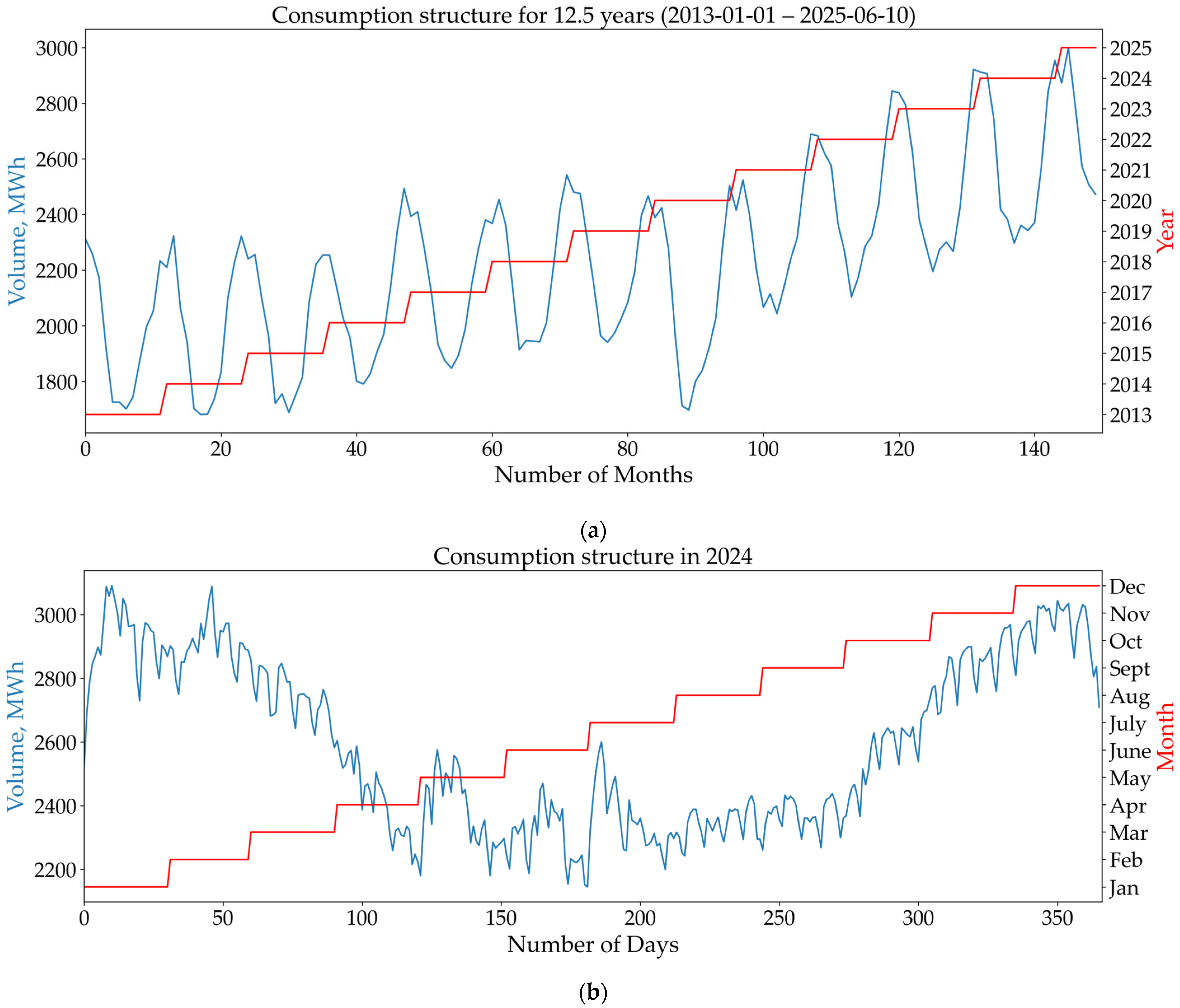
Figure 2a presents the monthly average electricity consumption structure of the analyzed ESC for the period from 1 January 2013 to 10 June 2025. The plot clearly demonstrates both an annual increasing trend in power consumption and the influence of seasonal factors. Furthermore, a significant consumption decline in 2020 is clearly observable, resulting from the COVID-19 pandemic’s economic impacts.

Figure 2b shows the daily average electricity consumption in 2024. The graph reveals an unusual sharp increase in energy consumption during May and July, which is atypical for this season. This increase is associated with the sudden temperature drop in May 2024 and the abnormally prolonged high temperatures in July 2024. Such unusual phenomena negatively affect the training quality and the generalization capability of STLF models.

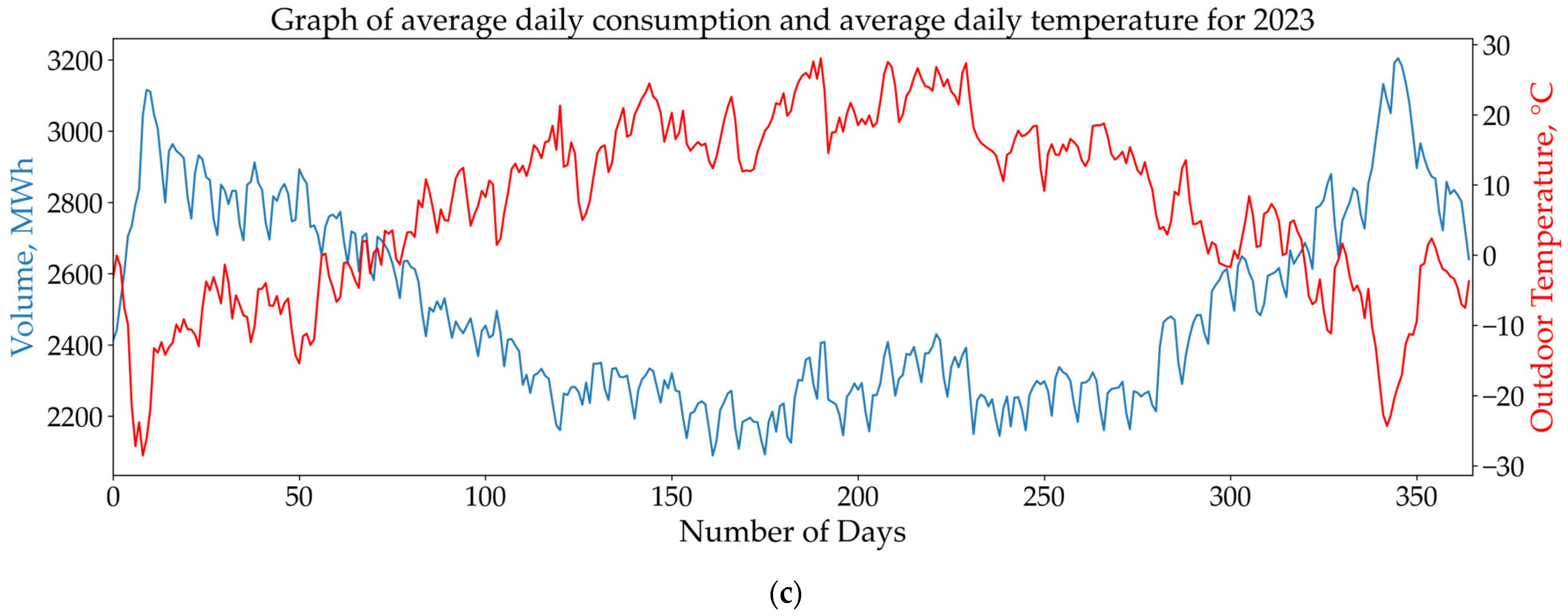
Figure 2c shows the relationship between average daily energy consumption and average daily temperature for 2023. As can be seen from the graph, energy consumption exhibits a strong seasonal dependence on ambient temperature. During summer months, there is a direct correlation due to an increased load on refrigeration equipment and ventilation systems, while in winter months, an inverse correlation is observed due to the demand for thermal energy and a higher load on heat-generating equipment.

Figure 3 shows the average daily energy consumption profile for May 2025. The graph clearly distinguishes weekdays, characterized by higher demand, from weekends and holidays (9 May), which are marked by reduced electricity consumption.

3.3. Data Preprocessing

Data preprocessing included the following steps:

• Day type encoding using the label encoder method: weekday—0, pre-holiday—1, holiday—2, and weekend—3. The encoding order was determined based on the decision tree algorithm’s requirements. The results were converted into a new feature, TypeDay.
• Splitting the Date parameter into separate features: Year (2013–2025), Month (1–12), Day (1–31), and Hour (0–23);
• Adding a WeekDay feature with days of the week: Monday—0, Tuesday—1, Wednesday—2, Thursday—3, Friday—4, Saturday—5, Sunday—6.
• Incorporating time lags for energy consumption from the previous 1 to 7 days: lag-1…lag-7. Since the first 168 records (24 × 7) in the database did not contain a complete set of time-lagged data, they were removed during preprocessing.
• Removing features: PredCons and PredGen for models trained on ActCons and ActGen, and ActCons and ActGen for models trained on PredCons and PredGen data.

The inclusion of lag-1…lag-7 features is essential because gradient-boosted trees, by nature, cannot inherently model temporal dependencies. Therefore, such lagged features are required to adapt to short-term demand change trends (e.g., spontaneous non-seasonal temperature drops, sharp declines in energy consumption due to unscheduled industrial load changes, etc.). The lag window size (24–168 h) was selected based on the planning horizon, following the approach in study [15].

Thus, the final dataset consisted of 17 features.

3.4. Model Selection and Hyperparameter Tuning

3.4.1. XGBoost Method

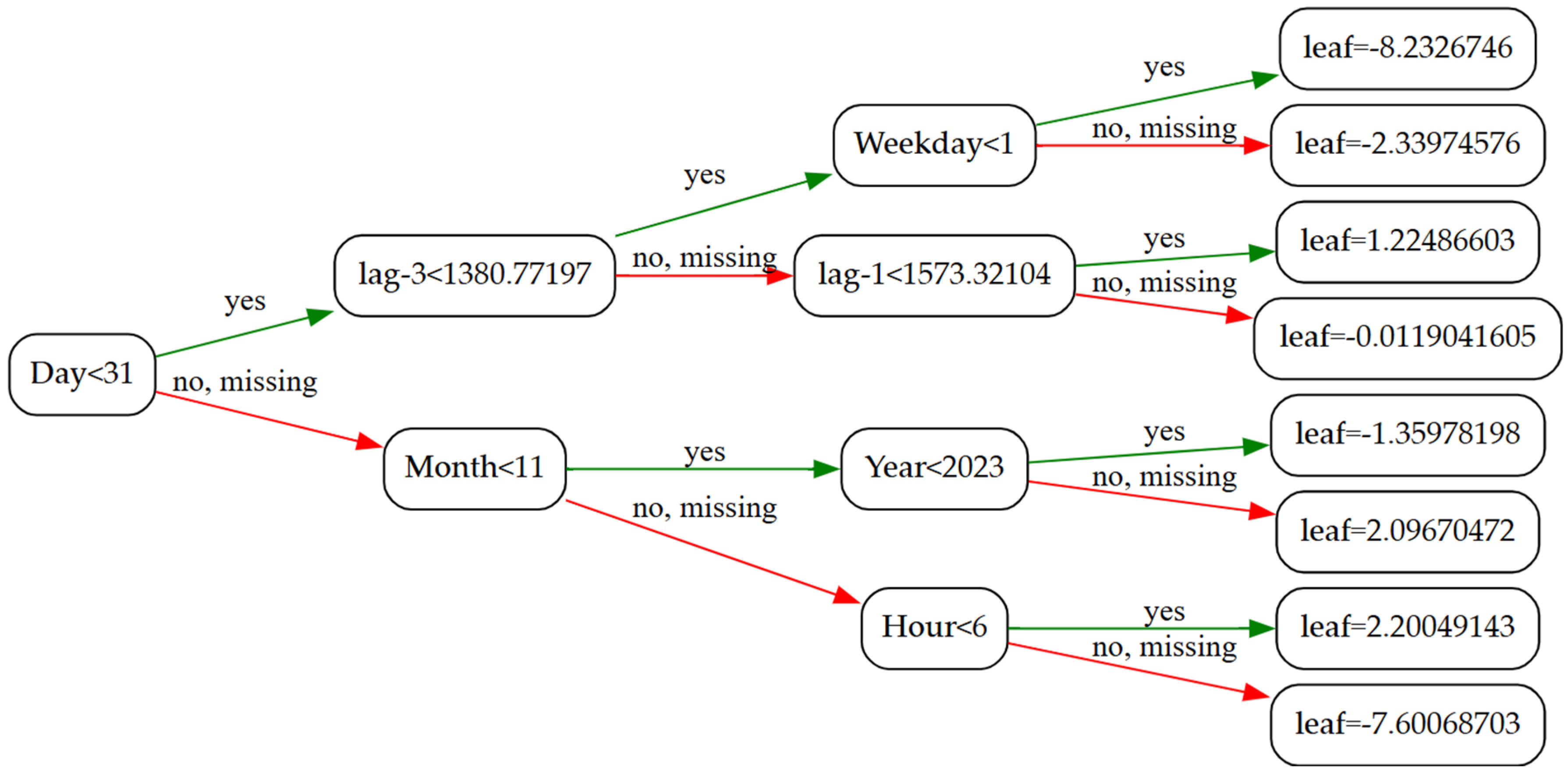
The XGBoost algorithm was used to develop the STLF models. This ensemble method is based on decision trees. Figure 4 shows an example of one such tree. Implementation details of the XGBoost method can be found in its official documentation [43].

The choice of the method was determined by the scalability and interpretability of its results. As highlighted by Zhao Q. et al. [5], Zhang, L., and Jánošík, D. [18], XGBoost is particularly well-suited for applications requiring detailed hourly electricity load forecasts.

As discussed in Section 2, the model’s upper performance bound depends primarily on data and feature quality. Model algorithms play only a secondary role in this context [11]. XGBoost serves as an excellent demonstration of this principle. To ensure clarity and wide reproducibility of the results, this study uses algorithms based on default XGBoost models.

3.4.2. List of Proposed Models

The list of proposed models was developed based on constraints imposed by data availability (Table 2).

First, BMI data was only available on the SO website starting from 29 November 2017, which led to us splitting the model development into two datasets: for the 2018–2025 period with BMI and for the 2013–2025 period without BMI. Second, ActGen and ActCons data in the region are published by the SO with a one-hour delay. This means that at the time of the DAM bid submission at 8:00 AM, only operational data up to 7:00 AM is available. In contrast, forecasted data (PredGen, PredCons, and BMI) is adjusted hourly and remains available until the end of the current day. Because of this, as an experiment, the model development was further divided into two additional dataset variants: with forecasted and with ActCons and ActGen data.

As a result, four STLF model models were proposed (

Table 3. List of and differences between the proposed STLF models.

Model	BEM Features	Period	XGBRegressor HP Tuning
br3_pred	PredGen, PredCons, Price	2018–2025	Adaptive re-training
br3_act	ActGen, ActCons, Price	2018–2025	Adaptive re-training
br3_act_LC	ActGen, ActCons, Price	2018–2025	Pre-tuned
br2_act_LC	ActGen, ActCons	2013–2025	Pre-tuned

).

3.4.3. Algorithms of the Proposed Models

• Model br3_pred

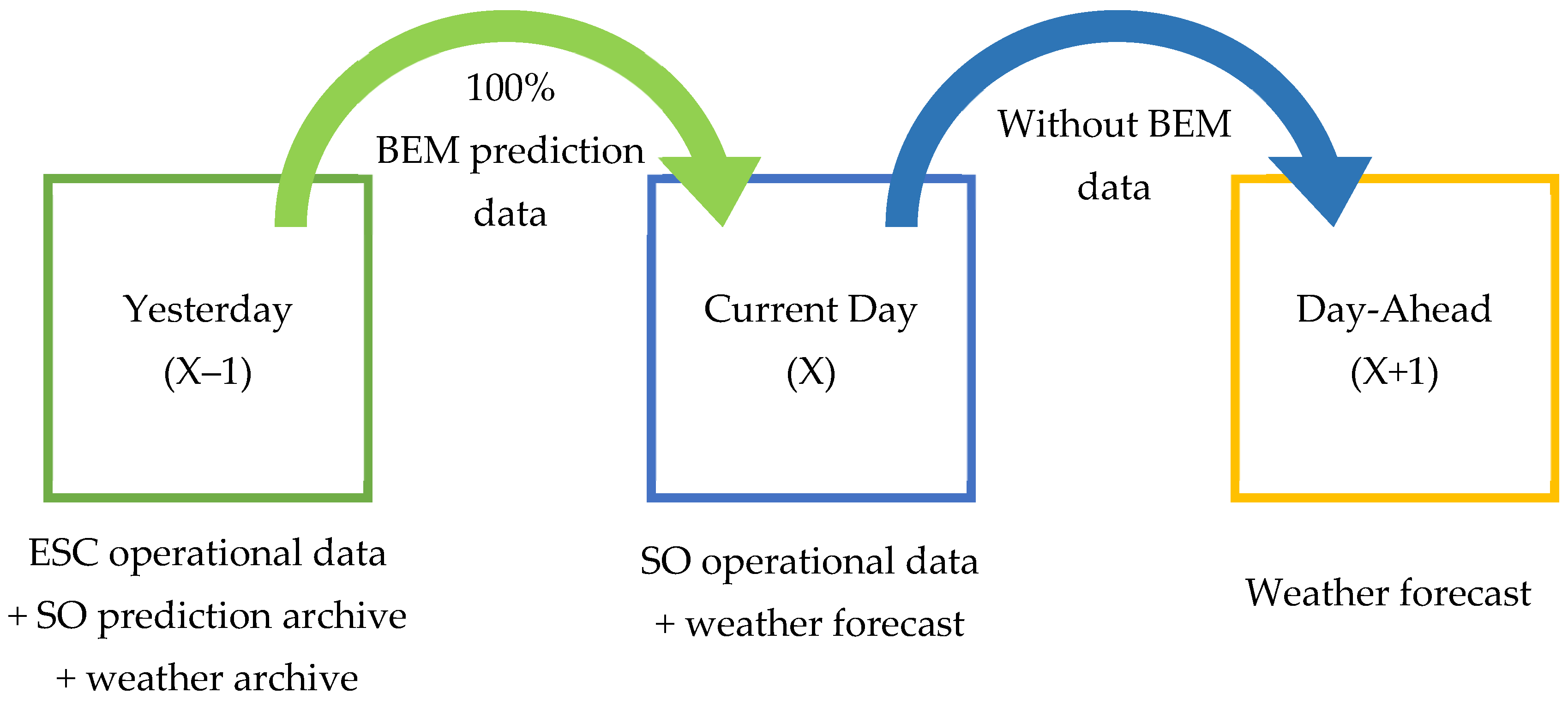
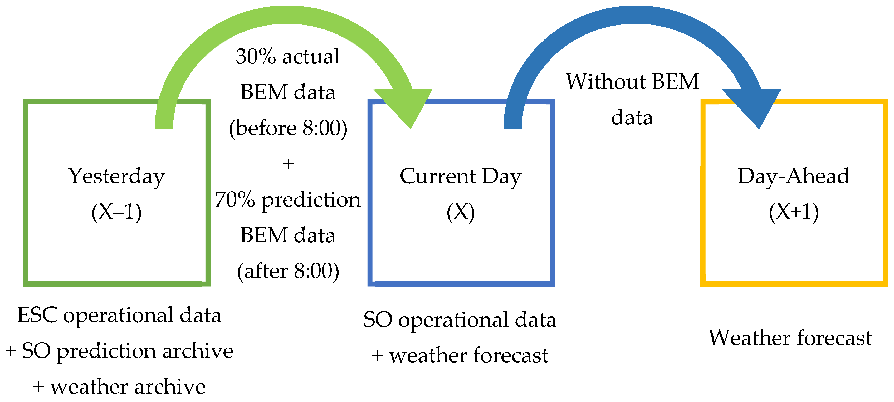
For ESCs, operational data on electricity consumption during the current trading day is only available for the previous day. Therefore, according to br3_pred model concept (Figure 5), ESC electricity consumption planning is first performed for the current day, and only then for the next day. Since the SO forecast is published before the end of the trading day, the forecast for the current day is made taking into account operational data from the balancing market (PredGen, PredCons, Price), while the forecast for the next day is performed without considering this data.

The advantage of this model is its simple and intuitive validation process. The drawback is that SO planning errors may negatively impact the model’s accuracy. Additionally, the SO may adjust its forecast after a day has passed, which could make the model validation results biased.

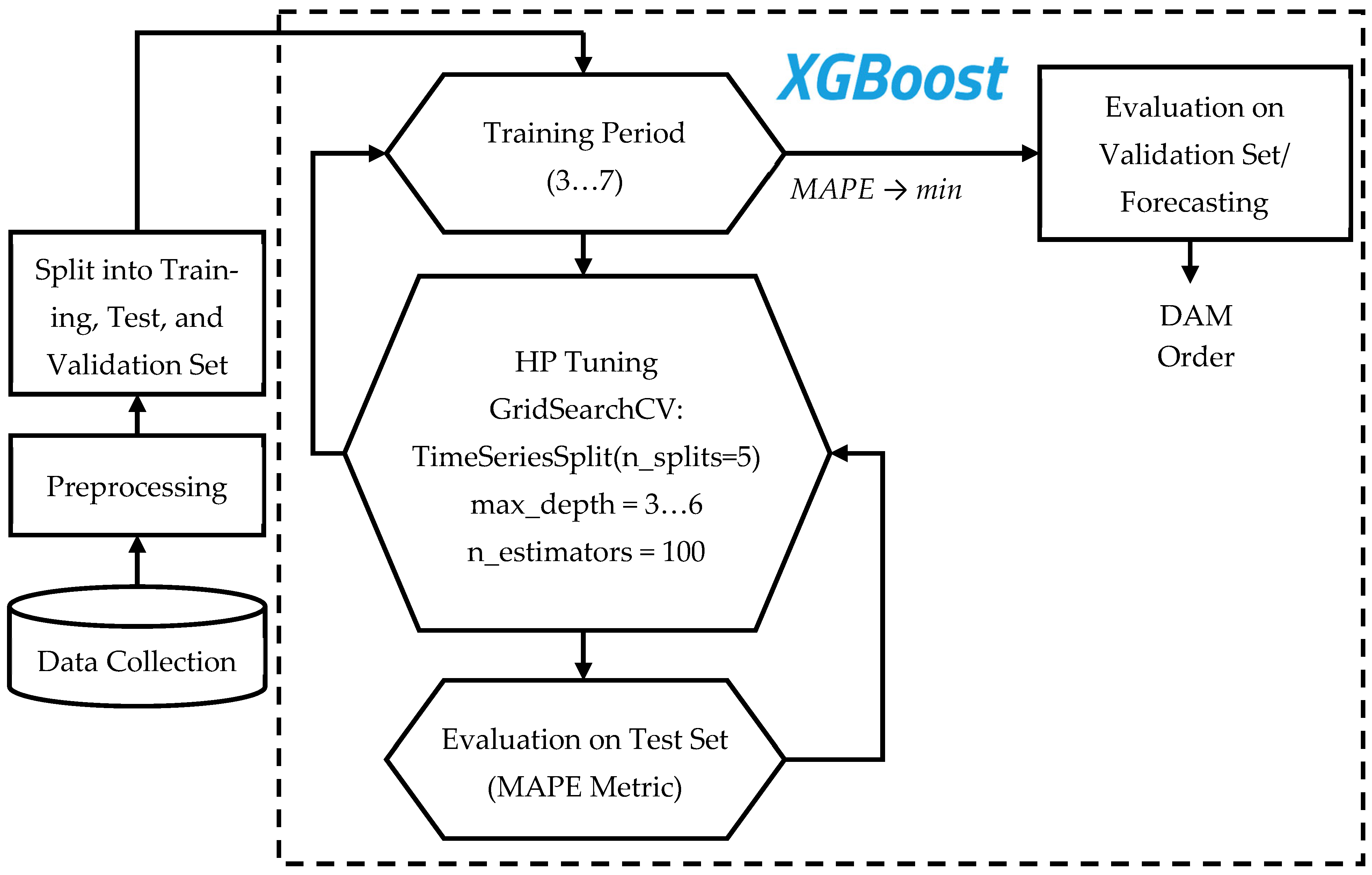
The algorithm for the br3_pred model is shown in Figure 6. After collection and preprocessing, the data is split into training, test, and validation sets. The test set period is set to one full year (365 days prior to the forecast/validation date), as this is the minimum timeframe that covers all seasonal patterns.

The model then proceeds with optimal parameter selection through a double-nested loop structure. At the upper level, the training period selected ranges from 3 years (2022–2024) to 7 years (2018–2024). At the lower level, hyperparameter tuning of the XGBoost regressor is performed through time-series cross-validation with a parameter grid (GridSearchCV utility, TimeSeriesSplit protocol). The cross-validation is configured with five data splits (n_splits = 5). To minimize algorithm complexity, the stack is built using only one parameter—max_depth (3–6). All other hyperparameters remain at their default settings. The MAPE metric is used as the model evaluation strategy.

The model with tuned parameters is then tested on a hidden validation dataset or used for forecast generation.

• Model br3_act

The key difference between the br3_act and br3_pred models lies in training on actual SO data (ActGen, ActCons, Price). Operational data is only available up to 7:00 AM at the time of DAM bid submission at 8:00 AM. Therefore, the missing actual data is replaced with forecasted values (Figure 7). The parameter tuning algorithm for the br3_act model remains completely identical to that of the br3_pred model (Figure 6).

This model offers two significant advantages. First, it minimizes the impact of SO planning errors on model accuracy, as training now utilizes actual rather than forecasted data. Second, it reduces uncertainty in current-day forecasting. Moreover, the later during the day the forecast is performed, the more actual data becomes available, consequently leading to progressively lower uncertainty.

The model’s drawback is that its validation process becomes significantly more complex, though this process gains greater objectivity.

• Model br3_act_LC

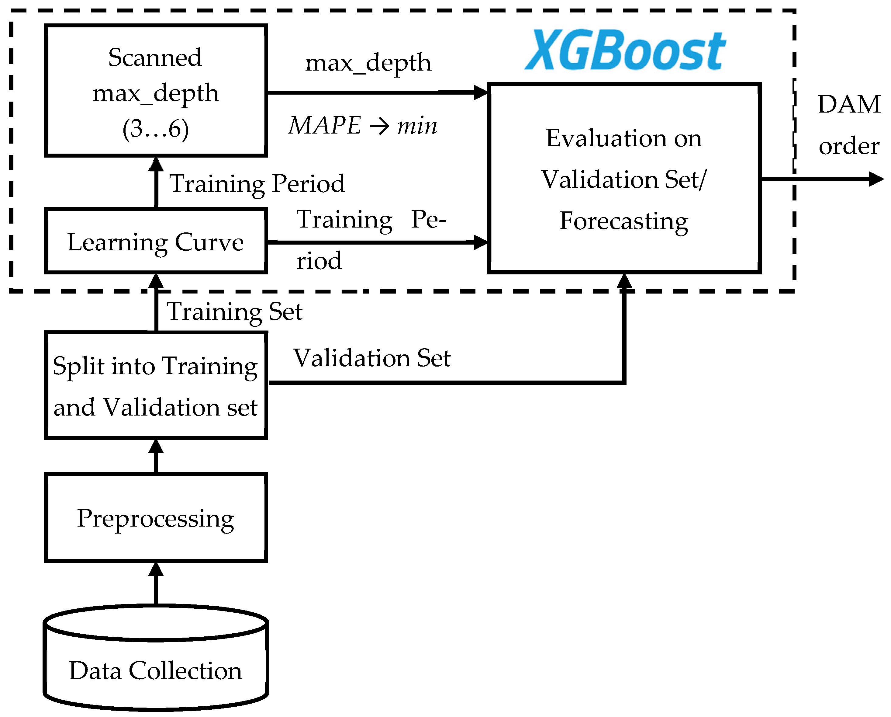
Conceptually, the br3_act_LC model is the same as the br3_act model (Figure 7). The only difference is in the model parameter tuning algorithm (Figure 8). Unlike the previous two models, the optimal training dataset size is determined in advance through a one-time procedure using the Scikit-learn Learning Curve tool. Similarly, the optimal decision tree depth is determined in advance and only once.

The key advantage of this model is its significantly reduced forecasting and validation time (τ) from 14.77 s/it to 1.97 s/it. Additionally, since the model parameters are pre-tuned, there is no need to allocate a separate test dataset. Therefore, the entire general dataset (2018–2025), excluding the validation set, can be used for model training, which enhances its generalization capability.

The main drawback of this model is the requirement for annual recalibration of the optimal training dataset size using Learning Curve, and quarterly adjustments of the regressor’s max_depth parameter.

• Model br2_act_LC

Conceptually and in terms of parameter tuning methodology, the br2_act_LC model is identical to the br3_act_LC model. The only distinction lies in the absence of the BMI (Price) parameter in the training dataset. As a result, the Learning Curve analysis is performed on the complete general dataset spanning 2013 to 2025.

3.5. Validation

3.5.1. Loss Functions and Metrics

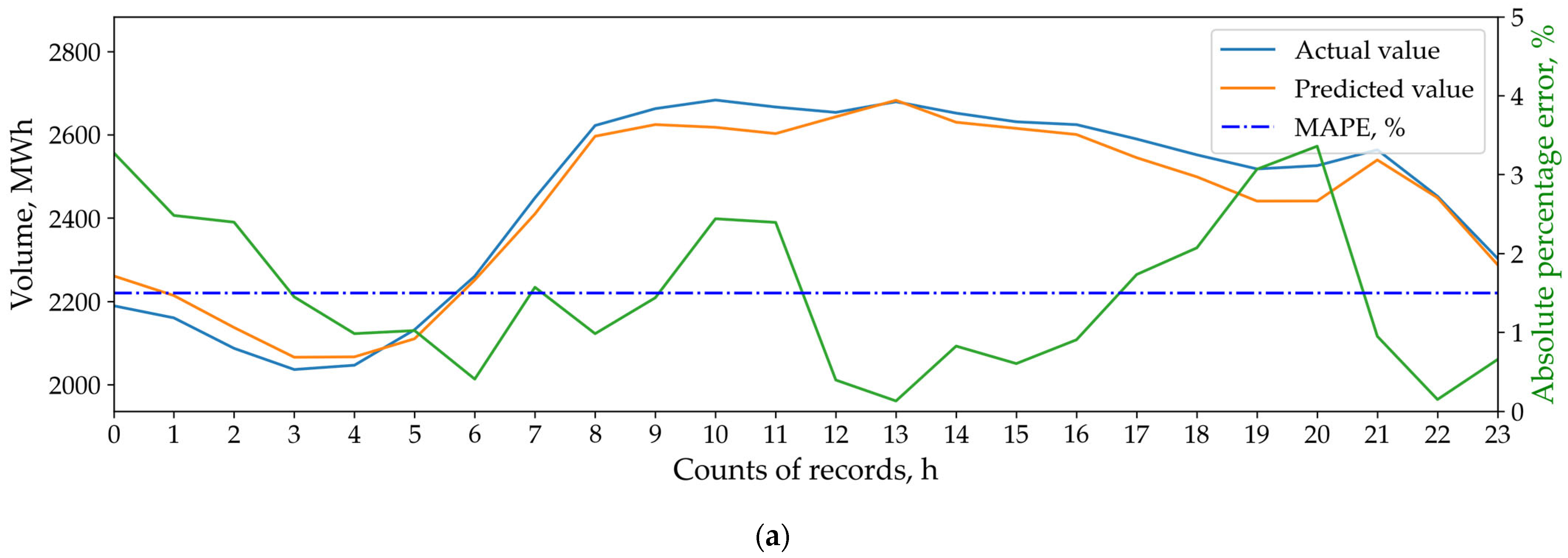
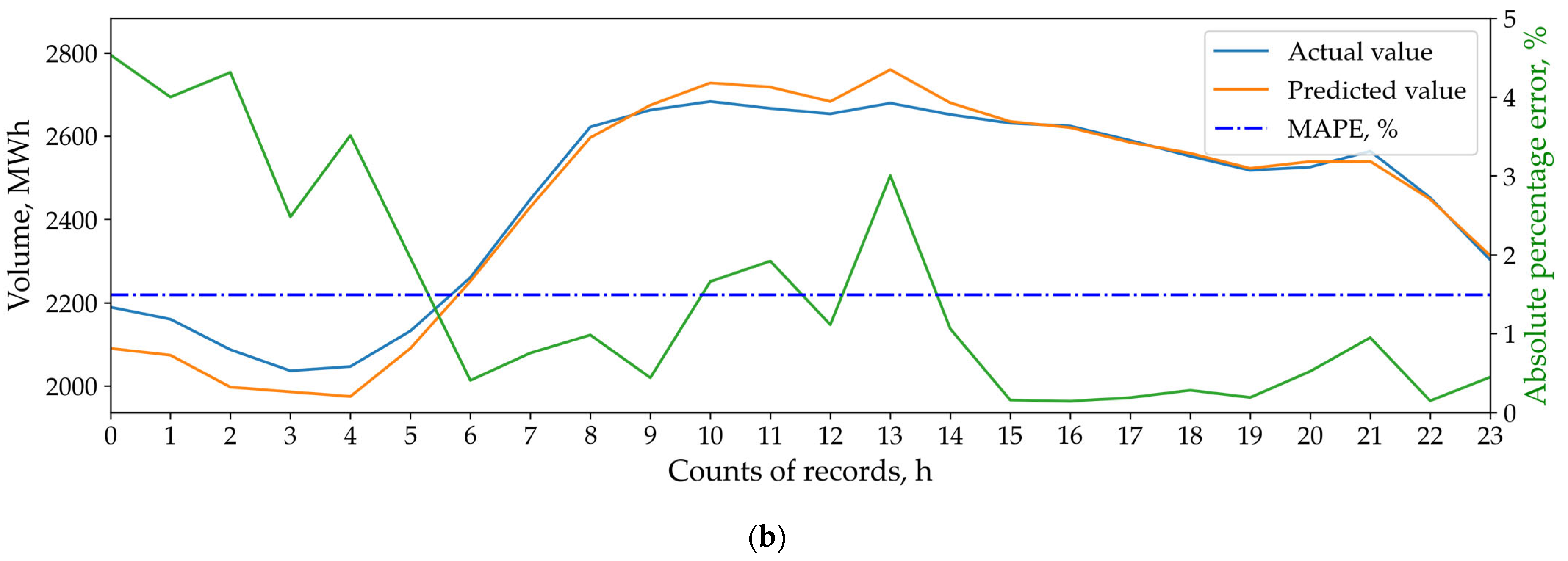
As mentioned in Section 2, the MAPE metric cannot adequately evaluate the commercial performance of the models. For example, Figure 9a,b show the daily validation results of two different models. In both cases, the MAPE metric equals 1.5%. However, in the first scenario (Figure 9a), downward forecast deviations are observed during peak consumption hours (8:00–12:00 and 16:00–21:00) when BEM tariffs reach their highest levels. In this case, upward deviations occur during off-peak hours (00:00–04:00) when penalties for underconsumption reach their maximum. In the second scenario (Figure 9b), downward deviations appear during system off-peak hours (00:00–06:00) when the price differential between DAM and BEM tends to zero. Conversely, upward deviations occur during system peak hours (09:00–15:00) when underconsumption penalties are minimal.

Clearly, the second model (Figure 9b) demonstrates greater commercial efficiency than the first (Figure 9a), though this advantage remains undetectable through MAPE metrics alone.

Therefore, the predictive accuracy of the developed STLF models was evaluated not only using standard metrics—MAE (1) and MAPE (2)—but also with three novel metrics:

• The Cumulative Financial Loss function of the Balancing Market (CLFBM), as follows:

  $$\mathrm{CLFBM}={\displaystyle \sum _{i=1}^n\left(\begin{array}{c}\left|A_i-P_i\right|\times T_{\mathrm{A}\_\mathrm{gr}\_\mathrm{P}},A_i>P_i\\ \left|A_i-P_i\right|\times T_{\mathrm{P}\_\mathrm{gr}\_\mathrm{A}},A_i\le P_i\end{array}\right)}$$

  (6)
• The Mean Financial Loss function of the Balancing Market (MLFBM), as follows:

  $$\mathrm{MLFBM}={\displaystyle \frac{1}{n}}\cdot {\displaystyle \sum _{i=1}^n\left(\begin{array}{c}\left|A_i-P_i\right|\times T_{\mathrm{A}\_\mathrm{gr}\_\mathrm{P}},A_i>P_i\\ \left|A_i-P_i\right|\times T_{\mathrm{P}\_\mathrm{gr}\_\mathrm{A}},A_i\le P_i\end{array}\right)}={\displaystyle \frac{\mathrm{CLFBM}}{n}}$$

  (7)
• The Median Financial Loss function of the Balancing Market (MedLFBM), as follows:

  $$\mathrm{MedLFBM}=\mathrm{Median}{\left[\begin{array}{c}\left|A_i-P_i\right|\times T_{\mathrm{A}\_\mathrm{gr}\_\mathrm{P}},A_i>P_i\\ \left|A_i-P_i\right|\times T_{\mathrm{P}\_\mathrm{gr}\_\mathrm{A}},A_i\le P_i\end{array}\right]}_{i=1\dots n}$$

  (8)

  where A_i and P_i are the actual and predicted values, respectively, and T_{A_gr_P} and T_{P_gr_A} are the BEM surcharges for overconsumption and BEM penalty for underconsumption against the plan (given in Section 3.1).

The CLFBM metric reflects the total financial losses on the BEM caused by model errors over a selected period (day, week, month, year, etc.). Its key advantage lies in providing highly interpretable results, enabling clear visual comparison of model performance when evaluated on the same validation dataset. The main limitation is its time-dependency, preventing direct comparisons between results obtained from validation datasets of different sizes.

The MLFBM metric represents the average hourly financial losses on the BEM due to model errors. Its primary benefit is time-independence, allowing comparison of validation results across datasets of varying sizes. A drawback of this metric is its low objectivity, as it is sensitive to error spikes that typically occur on weekends and holidays.

The MedLFBM metric represents median hourly financial losses on the BEM resulting from model errors. This metric was introduced specifically to assess the most frequently occurring losses, effectively evaluating financial impacts during typical weekday operations. By comparing the MedLFBM and MLFBM results, we can indirectly estimate the losses value during weekends and holidays. Its main limitation is reduced usefulness when analyzed in isolation from other metrics.

In the final dataset, the difference between actual and predicted values (A_i − P_i) is recorded in the “diff_cons” column, while the calculated losses (|A_i − P_i|× T) are stored in the “loss” column (Figure 10).

Notably, Figure 10 demonstrates how the MO utilizes tariff rates to manage demand during both peak load (6:00–7:00) and load decline (21:00–22:00) periods.

3.5.2. Validation Process Pipeline

The validation process pipeline is presented in Algorithm A1. This pipeline is common for all models, with all differences in validation dataset formation methods for models trained on predicted data (br3_pred) versus actual data (br3_act, br3_act_LC, br2_act_LC) being handled within the get_df_predicted() function.

At the beginning of validation, the validation dataset size is specified. Based on this selected size, the number of loop iterations is determined corresponding to the number of days in the dataset. The process then sequentially generates prediction dates: each iteration adds +1 day to the initial validation dataset date (line 2 of Algorithm A1). Using this date, the general population size is constrained to –2 days before the prediction date (line 3 of Algorithm A1). In other words, if the forecast is generated for 01.06.2025, the date and time in the last row of the constrained dataset should be 31.05.2025 0:00. Then the get_df_predicted() function is called, into which the limited population df_general_cut is passed as arguments: start date: prediction day—1 day (i.e., trading day); end date: prediction day (4th row of Algorithm A1). The get_df_predicted() function itself first generates a prediction for the trading day using the SO operational data (in our example, this covers 31.05.2025 1:00 ÷ 01.06.2025 0:00). Then, using this prediction, it generates a new prediction for the target prediction day (in our example, 01.06.2025 1:00 ÷ 02.06.2025 0:00). The get_df_predicted() function returns a 24-row dataframe containing prediction results for the date previously generated in the loop. This dataframe is appended to the previously generated empty frame df_result (line 1 of Algorithm A1). The loop continues iterating until all dates in the validation dataset are processed. Upon loop completion, the dataframe df_result merged with prediction values is combined with the validation sample df_validate by date (line 6 of Algorithm A1). The process then proceeds with comparing predicted versus actual values and calculating prediction metrics (line 7 of Algorithm A1).

Thus, we closely replicate real-world validation conditions where during the trading day, ESCs only have access to operational data from the previous day, while being required to make predictions for the next day.

The pipeline of the get_df_predicted() function for the br3_act model is presented in Algorithm A2.

3.6. Software and Hardware

The following software and libraries were used in this work: Python (v. 3.10.7), Pandas (v. 2.2.3), SKLearn (v. 1.4.2), XGBoost (v. 2.1.2), CatBoost (v. 1.2.8), Statsmodels (0.14.5), and SHAP (v. 0.47.0).

The calculations were carried out on the following hardware: CPU: Intel(R) Core(TM) i5-8300H; GPU: NVIDIA GeForce GTX 1050 Ti; RAM: DDR4, 16 GB.

4. Results

4.1. Exploratory Data Analisys

The exploratory data analysis focused on evaluating the significance of the initial features.

The first stage involved conducting correlation analysis of the data. The resulting Pearson correlation matrices (Figure 11) revealed that electricity demand (row Vol) shows strong dependence on the year and hour of consumption, outdoor air temperature, actual energy consumption, and total regional generation, as well as with the BMI (feature Price).

The strong correlation of demand with ActCons and ActGen in the region is explained by the fact that the consumer under study accounts for up to 40% of the total consumption structure of the UES of the Middle Volga (Section 3.1). Through its demand, the consumer directly influences the regional generation volumes and the BMI value. Therefore, despite their high correlation, these features must be retained as they are most sensitive to changes in demand trends.

Seasonal variations in feature relationships are insignificant, except for weather conditions (Figure 11). During summer, a noticeable positive correlation is observed between electricity production/consumption and outdoor temperature (Figure 11b). In winter, however, this relationship becomes significantly negative (Figure 11a).

The relationship between electricity demand and other features depending on the time of day is presented in Figure 12. As can be seen from the heatmap, between 6:00 and 18:00, the correlations between the target feature and the day of the week or day type strengthen. In other words, daytime consumption heavily depends on the day type: weekday, weekend, or holiday. During nighttime hours, the energy consumption remains relatively stable regardless of the day type.

The second stage involved evaluating feature importance within the XGBoost regressor context using both MDI (Mean Decrease in Impurity) and SHAP (SHapley Additive exPlanations) methods. According to the obtained results, the most valuable features for the regressor according to MDI assessment were the total ActCons in the region and the energy consumption at the same hour per day (lag-1) and per week (lag-7) before the prediction day (Figure 13). A similar distribution of the initial features was reported by Osgonbaatar, T. et al. [15] in their study.

Notably, the weight ratio between lag-7 and lag-1 features approximates 2:5. This can be explained by the decision tree’s tendency to primarily rely on the lag-1 feature when estimating weekday energy consumption, while shifting its dependence to the lag-7 feature during weekends (Saturday and Sunday).

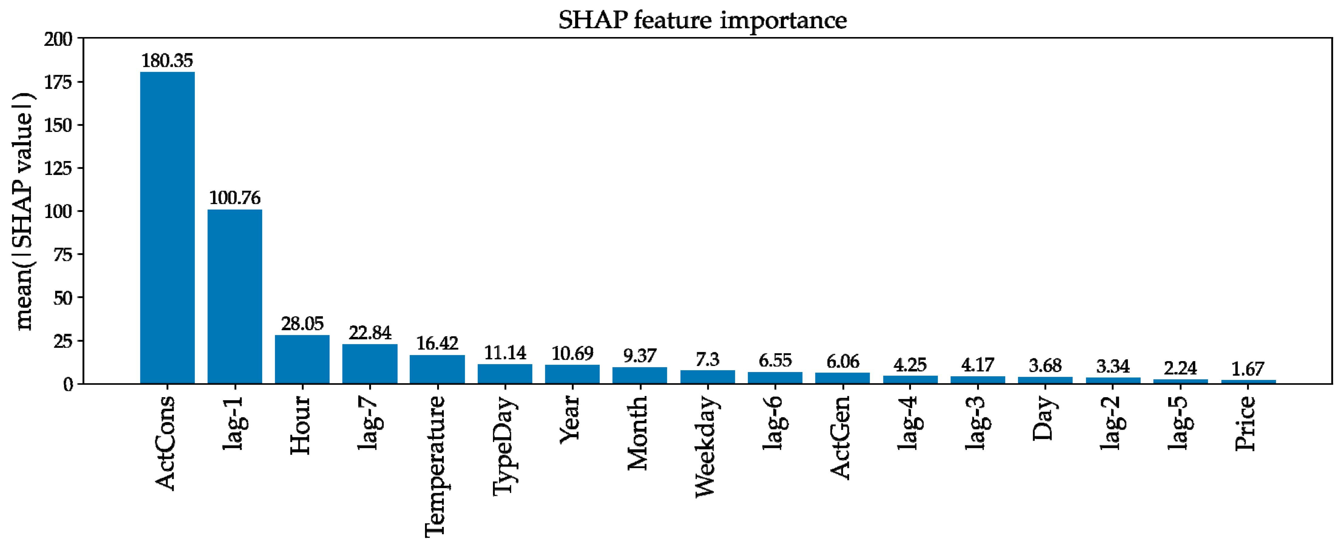
According to the SHAP analysis, in addition to ActCons, lag-7, and lag-1, the hour of consumption and outdoor temperature also represent important features (Figure 14).

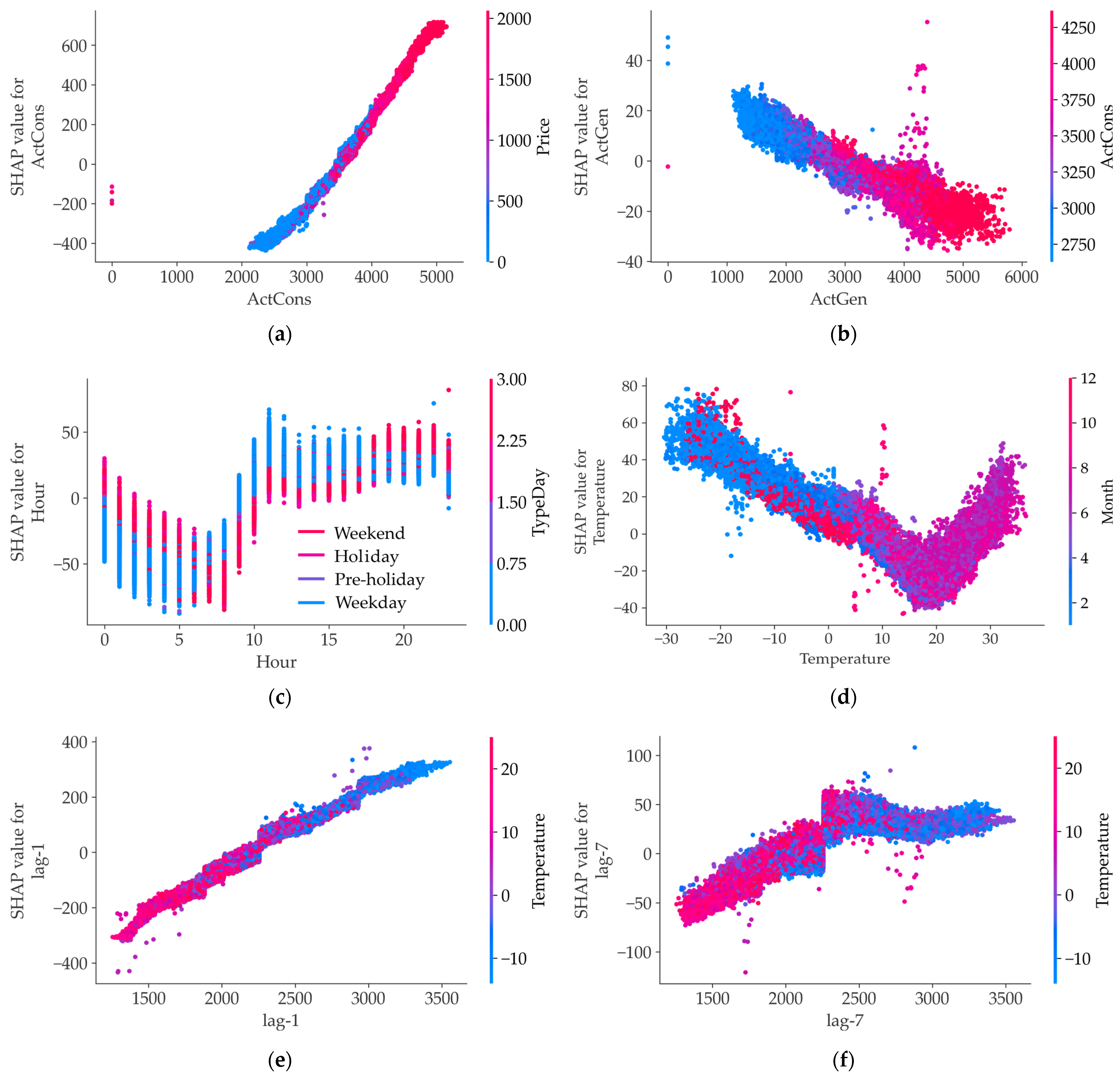
Figure 15 demonstrates how the most influential features affect the model’s behavior.

The relationships of ActCons (Figure 15a) and lag-1 (Figure 15e) with SHAP values exhibit a straight-line pattern with narrow point dispersion, indicating their linear positive influence on the predicted consumption volume. In contrast, an increased generation volume negatively affects SHAP values while consistently following the growth of ActCons (Figure 15b).

Figure 15a also demonstrates market mechanisms: energy consumption demand inevitably correlates with BMI growth.

The hour feature positively influences SHAP values during daytime hours and negatively during nighttime (Figure 15c). This effect intensifies on weekdays and weakens on weekends (except for the period from 18:00 to 24:00).

Energy consumption motivation is high during the daytime on weekdays, and during the nighttime on weekends or holidays.

The relationship between SHAP values and outdoor temperature demonstrates a dual nature (Figure 15d). During winter months, it shows a linear negative correlation. As temperatures rise and daylight duration increases, electricity consumption for heating and lighting decreases. The temperature’s influence on energy consumption minimizes at approximately 8 °C (the target heating season endpoint). Starting from approximately 18 °C (June–August), this relationship sharply reverses direction and becomes positive. This is explained by increased electricity consumption for refrigeration equipment and air conditioning operation.

The influence of lag-7 on SHAP values shows clear separation at 2300 MWh. At negative temperatures, this influence remains consistently positive, and vice versa. Thus, we observe an example of one of the conditions under which decision trees make determinations about increasing or decreasing SHAP values.

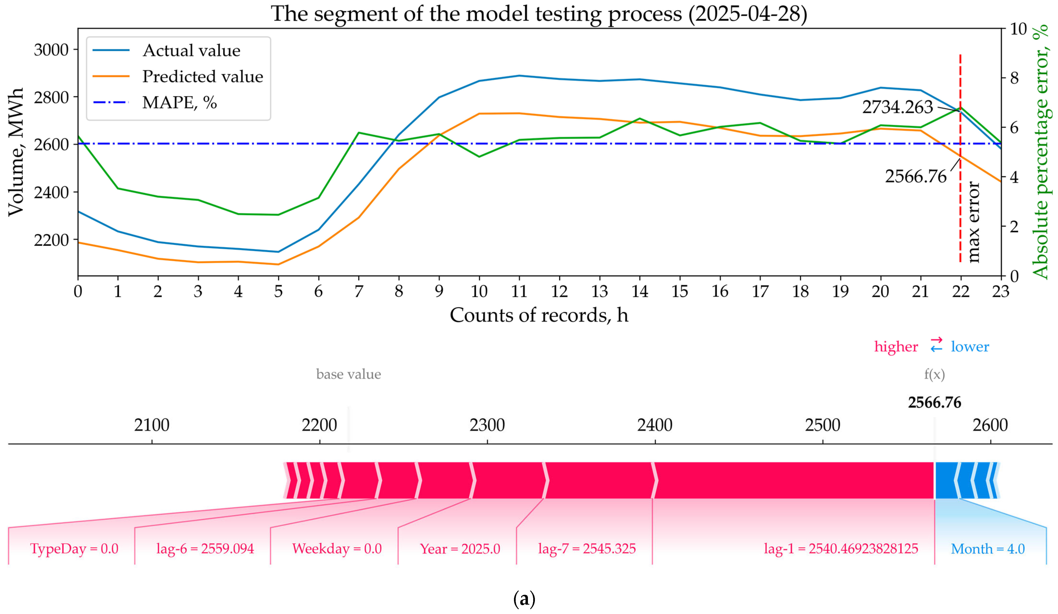
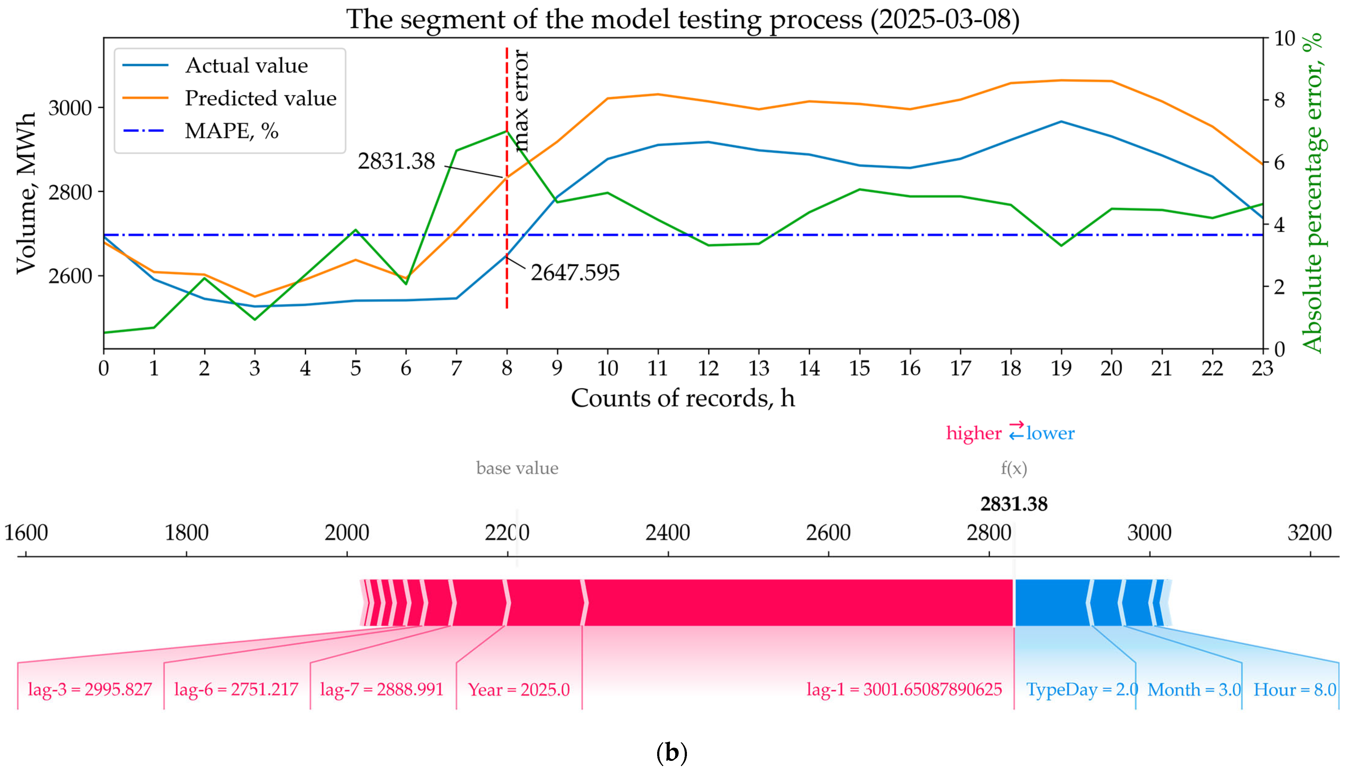
The third stage involved identifying specific feature patterns affecting financial losses. For this purpose, we used validation results from the br3_act model, which demonstrated the highest balancing costs (Section 4.3). From these results, we identified days with the largest deviations: actual exceeding planned consumption (28 April 2025, Figure 16a) and planned exceeding actual consumption (8 March 2025, Figure 16b). Subsequent analysis employed SHAP force plots to examine the contribution of individual features to the model’s prediction deviation on these specific days (Figure 16). It should be noted that the analysis excluded features such as ActCons, ActGen, and Price. The reason is that these data points are unknown at the time of making day-ahead predictions (Table 2, Figure 7), and therefore do not directly contribute to the final forecast outcome.

Force plots were created for hours with the maximum forecast deviation. In the first case (Figure 16a), the largest contributions to the predicted value (2566.76 MWh) came from features lag-1 (2540.47 MWh) and lag-7 (2545.325 MWh). Although they pushed the prediction from the Base Value in the correct direction, this proved insufficient to approach the actual energy consumption (2734.263 MWh). Only four features pushed the forecast downward—that is, in the incorrect direction—among which Month was the strongest. However, this influence was not substantial, and if completely eliminated, the forecast result would barely exceed 2600 MWh.

In the second case (Figure 16b), the largest contributions to the predicted value (2831.38 MWh) came from features lag-1 and Year. Since 8 March 2025 was a Saturday, it can be concluded that the model incorrectly assessed its most significant feature. The forecast result would have been more accurate if lag-7 (2888.991 MWh) had been chosen instead of lag-1 (3001.65 MWh), but it would still have remained far from the actual value (2647.595 MWh).

Thus, it can be concluded that the relationship between current and past energy consumption is not always stable, particularly during transitions between different day types.

4.2. Optimal Hyperparameters of the Model

As previously mentioned in Section 3.4.3, for the br3_pred and br3_act models, the optimal training period (training set size) and regressor tree depth (max_depth) were recalculated for each new prediction (or validation iteration) (Figure 6). This approach, while ensuring model adaptability to sudden data changes, concurrently increases computational duration.

In br3_act_LC and br2_act_LC models, such optimization was performed only once and in advance using the Learning Curve tool (Figure 17). The evaluation metric was set to negative mean absolute percentage error. The lines in the figure are the mean score value, and the shaded area around each lines indicate the variance of the model. According to the results, the optimal training period was determined to be 6 years for the br3_act_LC model (Figure 17a) and 10 years for the br2_act_LC model (Figure 17b). The observed error increase beyond these temporal boundaries suggests that older data loses relevance and merely introduces noise, ultimately degrading the models’ generalization performance. Both models demonstrated comparable performance on the test set, with similar mean error margins and variance: MAPE ≈ 1.5%.

The optimal tree depth for the models’ regressors was determined using Algorithm A1 and Algorithm A2 based on the identified training periods (

Table 4. The results of the optimal max_depth search.

br3_act_LC			br2_act_LC
Period, Year	Max_Depth	MAPE, %	Period, Year	Max_Depth	MAPE, %
6 1	3	1.507	10	3	1.507
	4	1.468		4	1.497
	5	1.457		5	1.447
	6	1.454		6	1.476

¹ Bolded values indicate the optimal hyperparameters of the model by the MAPE metric.

). For model br3_act_LC, max_depth = 6 was selected, while model br2_act_LC used max_depth = 5.

4.3. Model Validation Results

The validation results for all four models over the first five months of 2025 (1 January 2025 1:00 to 1 June 2025 0:00) are presented in

Table 5. Comparison of the prediction accuracy and commercial efficiency of the proposed models.

Month of 2025/ Model	MAPE, %
	XGBoost				CatBoost		ARIMA
	br3_pred	br3_act	br3_act_LC	br2_act_LC	br3_pred	br2_act_LC
January	1.605	1.576 1	1.640	1.636	1.616	1.827	11.248
February	1.233	1.246	1.196	1.242	1.154	1.194	11.446
March	1.169	1.181	1.104	1.122	1.190	1.221	10.091
April	1.689	1.619	1.570	1.490	1.710	1.596	11.567
May	1.610	1.609	1.618	1.548	1.744	1.770	11.023
Total
MAPE, %	1.464	1.449	1.429	1.411	1.488	1.527	11.062
MAE, MWh	39.912	39.346	38.992	38.487	40.341	41.396	277.585
CLFBM, RUR	15,961,596	17,237,366	16,409,259	16,726,062	16,557,290	17,005,792	138,535,705
MLFBM, RUR/h	4404.41	4756.45	4527.94	4615.36	4568.79	4692.55	38,227.29
MedLFBM, RUR/h	262.78	223.77	282.37	319.47	259.47	315.83	7271.8
τ, s/it	28.99	31.07	1.97	2.01	45.8	1.28	4.29

¹ Bolded values indicate the best results among all models.

. For comparison, validation results for the default ARIMA and CatBoost models have also been included.

According to Table 5, XGBoost models with pre-tuned hyperparameters demonstrated the best results in terms of both forecasting accuracy and computational performance. The br2_act_LC model achieved the lowest prediction error: MAPE = 1.411% and MAE = 38.487 MWh.

However, from the perspective of the Financial Loss function, the br3_pred model performed best, with CLFBM = 15,961,596, despite having the highest error metrics: MAPE = 1.464% and MAE = 39.912 MWh (Figure 18). This finding confirms our thesis from Section 2 regarding the insufficient objectivity of the MAPE metric.

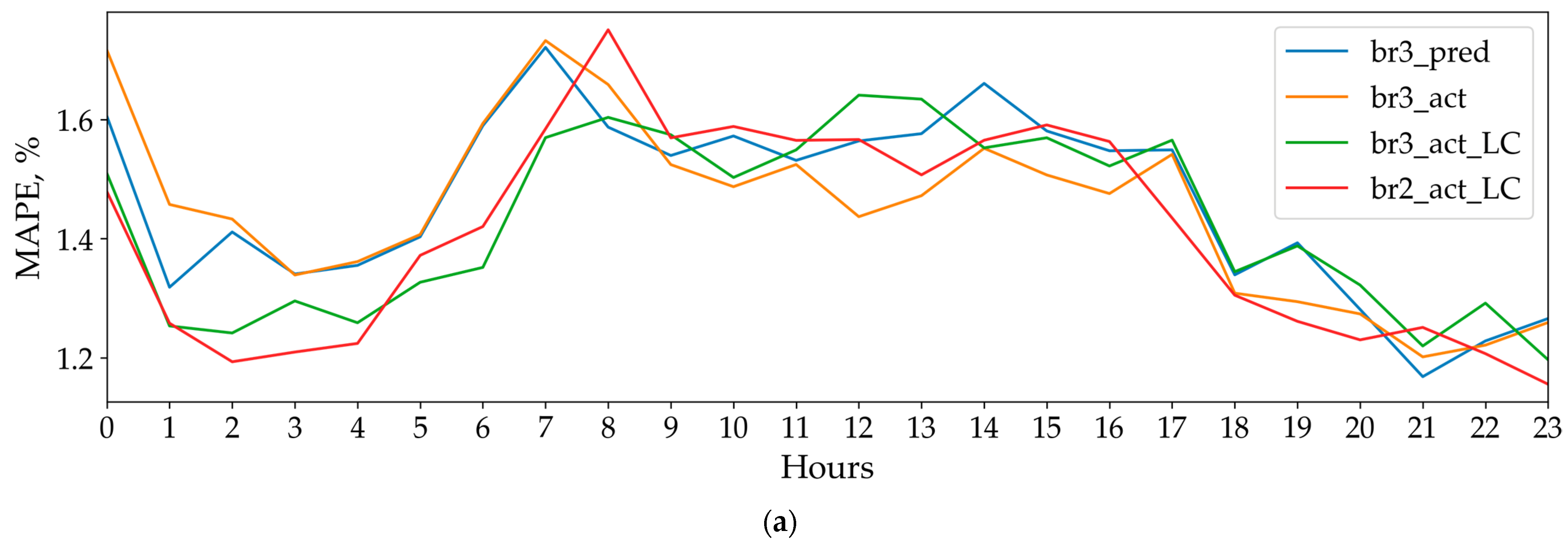
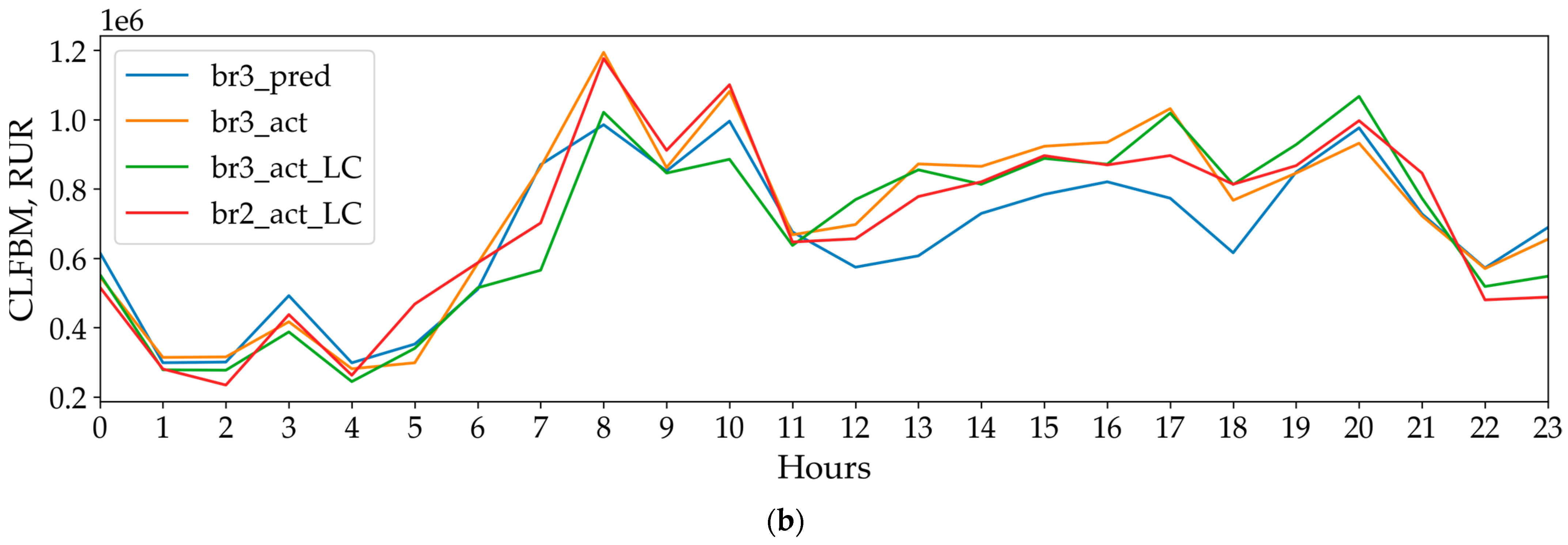
Unlike the MAE and MAPE metrics, CLFBM demonstrates greater sensitivity to forecasting errors during the most expensive peak electricity consumption hours (Figure 19).

For example, for the br2_act_LC model during the 2:00–8:00 period, the average MAPE increase is approximately 46% (from 1.2% to 1.75%, Figure 19a), while CLFBM increases by ~400% (Figure 19b). As another example, during the evening peak (17:00–20:00), when all models show decreasing MAPE values (Figure 19a), their actual balancing market costs rise and approach the morning maximum levels (Figure 19b).

Similar conclusions can be drawn regarding the sensitivity of the MLFBM metric (Figure 20). All the studied models demonstrate better performance on weekdays according to MAPE (Figure 20a), despite having the highest actual average hourly losses during these days (Figure 20b). Furthermore, all models perform worse on holidays than on weekends according to the MAPE metric. However, the MLFBM metric reveals that actual financial losses during these periods are comparable.

Based on the MLFBM and CLFBM metrics (Figure 20b,c), an objective conclusion can be reached: model error reduction should be prioritized for weekdays. Conversely, the MAPE metric does not enable such conclusions to be drawn.

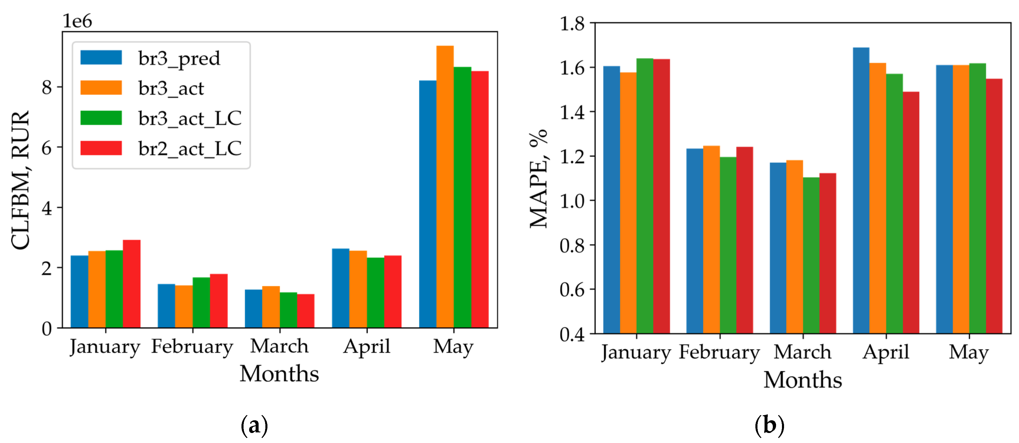
The analysis of CLFBM stability throughout the validation period months (Figure 21a) demonstrates noticeable seasonality in this metric. This phenomenon can be attributed to structural shifts in electricity consumption patterns occurring in late April to early May, corresponding to the end of the heating season in the Republic of Tatarstan.

The br3_act model exhibits the lowest MedLFBM (223.77) and highest MLFBM (4756.45) values (Table 5). This indicates that this model has the poorest generalization capability and, consequently, the highest financial balancing costs (Figure 18).

The br3_pred model demonstrates the smallest gap between the MLFBM and MedLFBM metrics (4141.63), confirming its superior generalization capability among all the proposed models.

The 15-fold increased computational performance of the br3_act_LC and br2_act_LC models (1.97 and 2.01 s/it, respectively), while being a secondary efficiency metric for this particular task, nevertheless enables faster and more cost-effective testing of both scientific and commercial hypotheses.

The br3_act model showed less impressive validation results. However, an adaptive re-training strategy was implemented for both the br3_act and br3_pred models, which may make them more accurate and commercially successful in the long term, particularly under significant electricity demand shifts.

5. Conclusions

STLF is an important and complex scientific–technical task. This study highlights the main problems of existing STLF models: weak interpretability, low commercial efficiency, poor scalability, and the insufficient objectivity of standard error metrics for their evaluation.

As a solution to these problems, this paper proposes ML models based on the XGBoost regressor, along with interpretation strategies for these models and new loss functions that incorporate the specifics of electricity market pricing.

The study results demonstrate that the model implementing the adaptive learning strategy achieves the best commercial efficiency, despite having the lowest accuracy and performance among the proposed models.

The study also notes that exogenous factors—specifically, the accuracy of meteorological forecasts and load forecasts provided by the SO for the UES—have the greatest impact on the model’s economic metrics. Therefore, for future work, we plan to extend the proposed approach to deep learning models such as N-BEATSx, NHITS, and TFT, which are capable of incorporating exogenous variables. This will allow us to validate the effectiveness of the proposed economic metrics and interpretation strategies on more advanced model families.

References

1. Dagoumas, A. Impact of Bilateral Contracts on Wholesale Electricity Markets: In a Case Where a Market Participant Has Dominant Position. Appl. Sci. 2019, 9, 382. [Google Scholar] [CrossRef]
2. Abbas, M.; Che, Y.; Khan, I.U. A Novel Stacked Ensemble Framework with the Kolmogorov-Arnold Network for Short-Term Electric Load Forecasting. Energy 2025, 332, 137216. [Google Scholar] [CrossRef]
3. Wholesale Market. Available online: https://en.np-sr.ru/srnen/abouttheelectricityindustry/electricityandcapacitymarkets/wholesalemarket/index.htm (accessed on 10 June 2025).
4. Sharifhosseini, S.M.; Niknam, T.; Taabodi, M.H.; Aghajari, H.A.; Sheybani, E.; Javidi, G.; Pourbehzadi, M. Investigating Intelligent Forecasting and Optimization in Electrical Power Systems: A Comprehensive Review of Techniques and Applications. Energies 2024, 17, 5385. [Google Scholar] [CrossRef]
5. Zhao, Q.; Wang, S.; Chen, Y.; Liu, J.; Sun, Y.; Su, T.; Li, N.; Fang, J. A hybrid framework for short-term load forecasting based on optimized InMetra Boost and BiLSTM. Energy 2025, 328, 136582. [Google Scholar] [CrossRef]
6. Karamolegkos, S.; Koulouriotis, D.E. Advancing short-term load forecasting with decomposed Fourier ARIMA: A case study on the Greek energy market. Energy 2025, 325, 135854. [Google Scholar] [CrossRef]
7. Liu, M.; Wang, J.; Deng, S.; Zhong, C.; Wang, Y. Short-term load probabilistic forecasting based on non-equidistant monotone composite quantile regression and improved MICN. Energy 2025, 320, 135339. [Google Scholar] [CrossRef]
8. Zhao, J.; Shen, X.; Liu, Y.; Liu, J.; Tang, X. Enhancing Aggregate Load Forecasting Accuracy with Adversarial Graph Convolutional Imputation Network and Learnable Adjacency Matrix. Energies 2024, 17, 4583. [Google Scholar] [CrossRef]
9. Wang, B.; Wang, L.; Ma, Y.; Hou, D.; Sun, W.; Li, S. A Short-Term Load Forecasting Method Considering Multiple Factors Based on VAR and CEEMDAN-CNN-BILSTM. Energies 2025, 18, 1855. [Google Scholar] [CrossRef]
10. Xu, F.; Wang, H.; Lu, Z.; Qiao, J.; Zhang, Y.; Heng, H. Research on Non-Intrusive Load Disaggregation Technology Based on VMD-Nyströmformer-BiTCN. Electronics 2024, 13, 4663. [Google Scholar] [CrossRef]
11. Ning, Z.; Jin, M.; Zeng, P. A Multimodal Interaction-Driven Feature Discovery Framework for Power Demand Forecasting. Energies 2025, 18, 2907. [Google Scholar] [CrossRef]
12. Ullah, K.; Ahsan, M.; Hasanat, S.M.; Haris, M. Short-term load forecasting: A comprehensive review and simulation study with CNN-LSTM hybrids approach. IEEE Xplore 2024, 12, 111858–111881. [Google Scholar] [CrossRef]
13. Gong, J.; Qu, Z.; Zhu, Z.; Xu, H.; Yang, Q. Ensemble Models of TCN-LSTM-LightGBM Based on Ensemble Learning Methods for Short-Term Electrical Load Forecasting. Energy 2025, 318, 134757. [Google Scholar] [CrossRef]
14. Yang, D.; Guo, J.-E.; Li, Y.; Sun, S.; Wang, S. Short-term load forecasting with an improved dynamic decomposition-reconstruction-ensemble approach. Energy 2023, 263, 125609. [Google Scholar] [CrossRef]
15. Osgonbaatar, T.; Matrenin, P.; Safaraliev, M.; Zicmane, I.; Rusina, A.; Kokin, S. A Rank Analysis and Ensemble Machine Learning Model for Load Forecasting in the Nodes of the Central Mongolian Power System. Inventions 2023, 8, 114. [Google Scholar] [CrossRef]
16. Chen, J.; Liu, L.; Guo, K.; Liu, S.; He, D. Short-Term Electricity Load Forecasting Based on Improved Data Decomposition and Hybrid Deep-Learning Models. Appl. Sci. 2024, 14, 5966. [Google Scholar] [CrossRef]
17. Luo, H.; Tong, C.; Gu, W.; Li, Z. Time-Series Imaging for Improving the Accuracy of Short-Term Load Forecasting. Energy 2025, 333, 137282. [Google Scholar] [CrossRef]
18. Zhang, L.; Jánošík, D. Enhanced short-term load forecasting with hybrid machine learning models: CatBoost and XGBoost approaches. Expert Syst. Appl. 2024, 241, 122686. [Google Scholar] [CrossRef]
19. Timur, O.; Üstünel, H.Y. Short-Term Electric Load Forecasting for an Industrial Plant Using Machine Learning-Based Algorithms. Energies 2025, 18, 1144. [Google Scholar] [CrossRef]
20. Zhou, B.; Wang, H.; Xie, Y.; Li, G.; Yang, D.; Hu, B. Regional short-term load forecasting method based on power load characteristics of different industries. Sustain. Energy Grids Netw. 2024, 38, 101336. [Google Scholar] [CrossRef]
21. Brahim, S.B.; Amayri, M.; Bouguila, N. One-day-ahead electricity load forecasting of non-residential buildings using a modified Transformer-BiLSTM adversarial domain adaptation forecaster. Comput. Intell. 2025, 13, 176. [Google Scholar] [CrossRef]
22. Ghimire, S.; Deo, R.C.; Casillas-Pérez, D.; Salcedo-Sanz, S. Electricity demand error corrections with attention bi-directional neural networks. Energy 2024, 291, 129938. [Google Scholar] [CrossRef]
23. Chen, C.; Yang, X.; Dai, X.; Chen, L. Short-term load forecasting based on different characteristics of sub-sequences and multi-model fusion. Comput. Electr. Eng. 2024, 120, 109675. [Google Scholar] [CrossRef]
24. Zhang, M.; Han, Y.; Zalhaf, A.S.; Wang, C.; Yang, P.; Wang, C.; Zhou, S.; Xiong, T. Accurate ultra-short-term load forecasting based on load characteristic decomposition and convolutional neural network with bidirectional long short-term memory model. Sustain. Energy Grids Netw. 2023, 35, 101129. [Google Scholar] [CrossRef]
25. Pavlatos, C.; Makris, E.; Fotis, G.; Vita, V.; Mladenov, V. Enhancing Electrical Load Prediction Using a Bidirectional LSTM Neural Network. Electronics 2023, 12, 4652. [Google Scholar] [CrossRef]
26. Pinto, T.; Praça, I.; Vale, Z.; Silva, J. Ensemble learning for electricity consumption forecasting in office buildings. Neurocomputing 2021, 423, 747–755. [Google Scholar] [CrossRef]
27. Sheng, Z.; An, Z.; Wang, H.; Chen, G.; Tian, K. Residual LSTM based short-term load forecasting. Appl. Soft Comput. 2023, 144, 110461. [Google Scholar] [CrossRef]
28. Han, X.; Shi, Y.; Tong, R.; Wang, S.; Zhang, Y. Research on short-term load forecasting of power system based on IWOA-KELM. Energy Rep. 2023, 9, 238–246. [Google Scholar] [CrossRef]
29. Stamatellos, G.; Stamatelos, T. Short-Term Load Forecasting of the Greek Electricity System. Appl. Sci. 2023, 13, 2719. [Google Scholar] [CrossRef]
30. Shahare, K.; Mitra, A.; Naware, D.; Keshri, R.; Suryawanshi, H.M. Performance analysis and comparison of various techniques for short-term load forecasting. Energy Rep. 2023, 9, 799–808. [Google Scholar] [CrossRef]
31. Wan, A.; Chang, Q.; Khalil, A.B.; He, J. Short-term power load forecasting for combined heat and power using CNN-LSTM enhanced by attention mechanism. Energy 2023, 282, 128274. [Google Scholar] [CrossRef]
32. Aguilar Madrid, E.; Antonio, N. Short-Term Electricity Load Forecasting with Machine Learning. Information 2021, 12, 50. [Google Scholar] [CrossRef]
33. Hasanat, S.M.; Ullah, K.; Yousaf, H.; Munir, K.; Abid, S. Enhancing Short-Term Load Forecasting With a CNN-GRU Hybrid Model: A Comparative Analysis. IEEE Xplore 2024, 12, 184132–184141. [Google Scholar] [CrossRef]
34. Sekhar, C.; Dahiya, R. Robust framework based on hybrid deep learning approach for short term load forecasting of building electricity demand. Energy 2023, 268, 126660. [Google Scholar] [CrossRef]
35. Ran, P.; Dong, K.; Liu, X.; Wang, J. Short-term load forecasting based on CEEMDAN and Transformer. Electr. Power Syst. Res. 2023, 214, 108885. [Google Scholar] [CrossRef]
36. Wei, N.; Yin, C.; Yin, L.; Tan, J.; Liu, J.; Wang, S.; Qiao, W.; Zeng, F. Short-term load forecasting based on WM algorithm and transfer learning model. Appl. Energy 2024, 353, 122087. [Google Scholar] [CrossRef]
37. Yamasaki, M.; Freire, R.Z.; Seman, L.O.; Stefenon, S.F.; Mariani, V.C.; dos Santos Coelho, L. Optimized hybrid ensemble learning approaches applied to very short-term load forecasting. Int. J. Electr. Power Energy Syst. 2024, 155, 109579. [Google Scholar] [CrossRef]
38. Asiri, M.M.; Aldehim, G.; Alotaibi, F.; Alnfiai, M.M.; Assiri, M.; Mahmud, A. Short-term load forecasting in smart grids using hybrid deep learning. IEEE Access 2024, 12, 23504–23513. [Google Scholar] [CrossRef]
39. Tarmanini, C.; Sarma, N.; Gezegin, C.; Ozgonenel, O. Short term load forecasting based on ARIMA and ANN approaches. Energy Rep. 2023, 9, 550–557. [Google Scholar] [CrossRef]
40. Dong, J.; Jiang, Y.; Chen, P.; Li, J.; Wang, Z.; Han, S. Short-term power load forecasting using bidirectional gated recurrent units-based adaptive stacked autoencoder. Int. J. Electr. Power Energy Syst. 2025, 165, 110459. [Google Scholar] [CrossRef]
41. Cavus, M.; Allahham, A. Spatio-Temporal Attention-Based Deep Learning for Smart Grid Demand Prediction. Electronics 2025, 14, 2514. [Google Scholar] [CrossRef]
42. Ali, A.; Naeem, H.Y.; Sharafian, A.; Qiu, L.; Wu, Z.; Bai, X. Dynamic multi-graph spatio-temporal learning for citywide traffic flow prediction in transportation systems. Chaos Solitons Fractals 2025, 199, 116898. [Google Scholar] [CrossRef]
43. XGBoost Tutorials. Introduction to Boosted Trees. Available online: https://xgboost.readthedocs.io/en/stable/tutorials/model.html (accessed on 10 June 2025).
Figure 1. Energy market sequence [3].
Energies 18 05144 g001
Figure 2. Electricity consumption structure: averaged by month (a); annual, averaged by days (b); annual, averaged by days, with dependence on daily mean temperature (c).
Energies 18 05144 g002aEnergies 18 05144 g002b
Figure 3. Hourly energy consumption profile for May 2025.
Energies 18 05144 g003
Figure 4. Example of decision tree of XGB model.
Energies 18 05144 g004
Figure 5. br3_pred model concept.
Energies 18 05144 g005
Figure 6. Parameter tuning algorithm for br3_pred and br3_act models.
Energies 18 05144 g006
Figure 7. Concept of br3_act, br3_act_LC, and br2_act_LC models.
Energies 18 05144 g007
Figure 8. Parameter tuning algorithm for br3_act_LC and br2_act_LC models.
Energies 18 05144 g008
Figure 9. Comparison of validation results for two different STLF models: br3_act (a); br3_pred (b).
Energies 18 05144 g009aEnergies 18 05144 g009b
Figure 10. Graphical representation of a sample from the final dataset with the calculated economic metrics.
Energies 18 05144 g010
Figure 11. Seasonal stratification: winter (a); summer (b).
Energies 18 05144 g011
Figure 12. Hour-of-day correlation heatmaps.
Energies 18 05144 g012
Figure 13. Feature importance.
Energies 18 05144 g013
Figure 14. Feature importance for SHAP.
Energies 18 05144 g014
Figure 15. SHAP value dependence for ActCons (a), ActGen (b), Hour (c), Temperature (d), lag-1 (e), and lag-7 (f).
Energies 18 05144 g015
Figure 16. SHAP force plots for max diff actual and predicted values (a), and max diff predicted and actual values (b).
Energies 18 05144 g016aEnergies 18 05144 g016b
Figure 17. Learning curve for br3_act_LC (a) and br2_act_LC (b).
Energies 18 05144 g017
Figure 18. Ranking of XGBoost models.
Energies 18 05144 g018
Figure 19. Hour of day sensitivity for metrics MAPE (a) and CLFBM (b).
Energies 18 05144 g019aEnergies 18 05144 g019b
Figure 20. Type-of-day sensitivity for metrics MAPE (a), MLFBM (b), and CLFBM (c).
Energies 18 05144 g020
Figure 21. Seasonal stability analysis for CLFBM (a) and MAPE (b).
Energies 18 05144 g021