Article

Electric Vehicle Energy Management Under Unknown Disturbances from Undefined Power Demand: Online Co-State Estimation via Reinforcement Learning

by
C. Treesatayapun
1,*,
A. D. Munoz-Vazquez
2,
S. K. Korkua
3,
B. Srikarun
3 and
C. Pochaiya
3
1
Robotics and Advanced Manufacturing, Center for Research and Advanced Studies (CINVESTAV), 1062 Industria Metalurgica Av., Ramos Arizpe 25903, Mexico
2
Higher Education Center at McAllen, Texas A&M University (TAMU), College Station, TX 78504, USA
3
School of Engineering and Technology, Walailak University, Nakhonsrithammarat 80161, Thailand
*
Author to whom correspondence should be addressed.
Energies 2025, 18(15), 4062; https://doi.org/10.3390/en18154062 (registering DOI)
Submission received: 4 July 2025 / Revised: 25 July 2025 / Accepted: 29 July 2025 / Published: 31 July 2025
(This article belongs to the Special Issue Forecasting and Optimization in Transport Energy Management Systems)

Abstract

This paper presents a data-driven energy management scheme for fuel cell and battery electric vehicles, formulated as a constrained optimal control problem. The proposed method employs a co-state network trained using real-time measurements to estimate the control law without requiring prior knowledge of the system model or a complete dataset across the full operating domain. In contrast to conventional reinforcement learning approaches, this method avoids the issue of high dimensionality and does not depend on extensive offline training. Robustness is demonstrated by treating uncertain and time-varying elements, including power consumption from air conditioning systems, variations in road slope, and passenger-related demands, as unknown disturbances. The desired state of charge is defined as a reference trajectory, and the control input is computed while ensuring compliance with all operational constraints. Validation results based on a combined driving profile confirm the effectiveness of the proposed controller in maintaining the battery charge, reducing fluctuations in fuel cell power output, and ensuring reliable performance under practical conditions. Comparative evaluations are conducted against two benchmark controllers: one designed to maintain a constant state of charge and another based on a soft actor–critic learning algorithm.

1. Introduction

The growing demand for sustainable transportation has intensified research in electric vehicles powered by hybrid energy sources [1]. Among these, fuel cell and battery electric vehicles represent a promising solution by combining the high energy density of hydrogen fuel cells with the fast dynamic response of lithium-ion batteries [2,3]. Effective coordination of power flow between these energy sources is critical to achieving performance, efficiency, and durability optimization objectives [4,5]. A key challenge is the development of an energy management system (EMS) that can optimize fuel cell operation while maintaining the battery state of charge within acceptable bounds [6,7]. Conventional energy management strategies often rely on rule-based logic or predictive control methods that depend on accurate models of the vehicle powertrain [8,9]. However, precise modeling of such systems is inherently difficult due to nonlinear dynamics, time-varying operating conditions, and the presence of unknown or uncertain elements, such as auxiliary loads and environmental factors. Moreover, many model-based approaches require prior knowledge of future driving profiles or disturbance patterns, which may not be readily available in real-time applications [10,11].
Model-based EMS for electric vehicles typically rely on detailed mathematical representations of powertrain components, including fuel cells, batteries, electric motors, and auxiliary loads [12,13]. These models facilitate the application of advanced optimization and control techniques, such as model predictive control and dynamic programming, to compute power allocation strategies that improve energy efficiency and prolong component lifespan [14]. By accurately capturing system dynamics and constraints, model-based EMS can predict future states and proactively regulate power flow [15]. However, the performance of these approaches is highly dependent on the accuracy and completeness of the underlying models, which are often difficult to construct due to nonlinear behavior, parameter uncertainties, and variable operating conditions [16]. In addition, the computational demands associated with solving model-based optimization problems in real time may hinder practical implementation, especially under uncertain or rapidly changing environments [17].
The application of reinforcement learning (RL) to EMS in electric vehicles has gained substantial momentum, driven by the increasing need to manage system complexity and uncertainty without reliance on precise mathematical models [18,19]. In particular, actor–critic frameworks have emerged as a promising class of RL algorithms, as they integrate the processes of value estimation and policy optimization, thereby supporting real-time adaptability to dynamic driving environments and power demand fluctuations [20,21]. Compared to traditional control strategies such as rule-based logic or model predictive control (MPC), actor–critic methods have demonstrated superior performance in capturing nonlinear behaviors and learning optimal control policies through direct interaction with the system [22]. Despite these advantages, conventional RL implementations often rely on pretraining with large and diverse datasets, which can constrain their practicality for real-time deployment [23,24]. Moreover, the inherent dimensional complexity of electric vehicle powertrain systems—characterized by high-dimensional state-action spaces—poses challenges related to computational overhead and algorithmic convergence [25,26]. These limitations have motivated the development of more computationally efficient and data-adaptive approaches that can learn effectively in online settings without extensive offline training.
In response to the limitations of model-based methods and conventional actor–critic architectures, data-driven and model-free control approaches have attracted increasing interest due to their ability to learn system behavior directly from real-time measurements [27]. These methods offer robust adaptability under uncertain and varying conditions without relying on explicit system models. This work proposes an adaptive control framework based on a fuzzy rule emulated network, termed MiFREN [28], for real-time power management in fuel cell and battery electric vehicles. The scheme incorporates two learning networks: MiFRENm, which estimates unknown system dynamics, and MiFRENs, which approximates the cost gradient necessary for control optimization. Together, these networks enable online adaptation and optimization without prior knowledge of system parameters.
The main contributions of this work are summarized as follows:
  • Unlike conventional reinforcement learning schemes [21,22,23], which typically rely on iterative learning and extensive offline training, the proposed approach employs a co-state network that is trained solely using online data in real time. This design enables the formulation of an optimal energy management controller without requiring a comprehensive dataset or prior knowledge of the entire operational domain. Additionally, the framework inherently avoids the curse of dimensionality, making it well-suited for practical deployment in embedded systems.
  • By treating power consumption associated with air conditioning systems, time-varying slopes and road conditions, passenger support systems, and other onboard demands as unknown disturbances, the robustness of the proposed scheme is demonstrated both from a practical perspective and through theoretical analysis.
  • From the perspective of energy management as a control system, the desired state of charge (SOC) is formulated as the reference trajectory, while the optimal control input is computed using the proposed control law under full operational constraints.
The remainder of this paper is organized as follows. Section 2 presents the problem formulation, where the electric vehicle with energy management is modeled as a class of discrete-time systems, and the optimal solution is addressed from the perspective of a model-free control approach. Section 3 details the design of the proposed controller along with the corresponding analysis. Section 4 provides validation results and comparative evaluations. Finally, the conclusion is presented in Section 5.

2. Problem Formulation with EV-EMS Framework

2.1. A Class of Control Systems Based on Model-Free EV-EMS

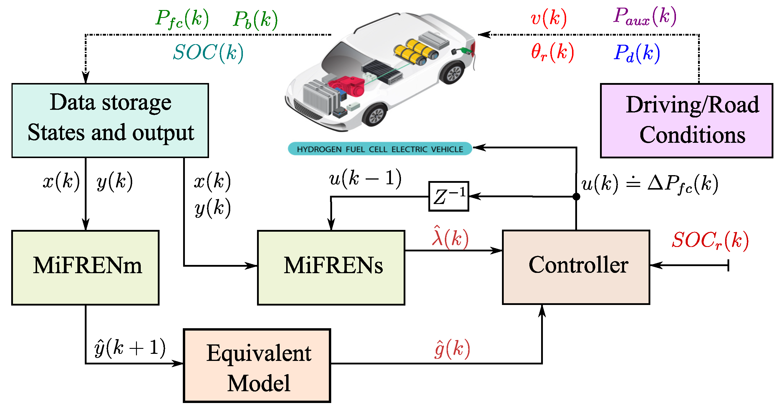
For the purposes of this study, the fuel cell/battery electric vehicle is, without loss of generality and within a discrete-time aspect, briefly represented by the power-flow block diagram shown in Figure 1. The drive block denotes the required power P d ( k ) [kW] at sampling index k, as determined by the vehicle velocity v ( k ) , physical resistances, and longitudinal dynamics.
In this work, the standard model is employed to express the power as a function of the real-time sampling index k and sampling interval T s [s] as
P d ( k ) = 1 2 C d A f ρ a v 3 ( k ) + R i m 0 v ( k ) v ( k ) v ( k 1 ) T s + m 0 g v ( k ) sin ( θ r ( k ) ) + R r m 0 g v ( k ) sin ( θ r ( k ) ) ,
where θ r ( k ) denotes the road slope and other parameters are defined as Table 1.
With respect to a quasi-static fuel cell model, P f c ( k ) [kW] denotes the power output at sampling index k, which reflects the instantaneous hydrogen consumption, expressed as m ˙ H 2 ( k ) = f f c ( P f c ( k ) ) , where f f c ( ) is a generally nonlinear function considered unknown in this work. In light of this relationship, and consistent with insights from related studies, the EMS design in this work is directly based on the principle that a reduction in the required power P f c ( k + 1 ) leads to a corresponding decrease in hydrogen consumption.
The lithium-ion battery pack is modeled using its standard equivalent circuit, where the output current I b ( k ) is governed by the battery power P b ( k ) , such that
I b ( k ) = V o c V o c 2 4 R i P b ( k ) 2 R i ,
where V o c is the open circuit voltage and R i is the internal resistance. It is evident that under discharge conditions, when P b ( k ) < V o c 2 4 R i , a proportional relationship between the battery power and output current can be established, provided that the state variation is consistent with the direction of the discharge current. By this mean, the change in S O C or S O C ˙ can be discretized as
S O C ˙ | t [ k T s , ( k + 1 ) T s ) S O C ( k + 1 ) S O C ( k ) T s = η b sign P b ( k ) P b ( k ) 3 , 600 E 0 ,
or
S O C ( k + 1 ) = S O C ( k ) η b sign P b ( k ) P b ( k ) 3 , 600 E 0 T s ,
where η b denotes the Coulombic efficiency of the battery pack, and E o represents its capacity, as specified in Table 1.
The auxiliary power P a u x ( k ) accounts for the total power consumption associated with the air conditioning system, passenger support utilities, operational functions, and other onboard loads. In this work, P a u x ( k ) is treated as an unknown disturbance, and, in contrast to previous works, no estimation models or observers are employed.
The electric motor, integrated into the EV powertrain, has an efficiency η e m generally characterized as a function of the output torque τ m and rotational speed ω m , such that η e m = f η e m ( τ m , ω m ) , with f η e m ( · ) defined experimentally. For simplicity and without loss of generality, η e m is specified as listed in Table 1. The motor is driven via a DC/AC inverter and a mechanical transmission, with their respective efficiencies denoted by η D C / A C and η m , also provided in Table 1. Furthermore, the electrical energy generated by the fuel cell is delivered through a DC/DC converter, with its efficiency η D C / D C likewise specified. Based on these considerations, the power balance for the EV powertrain can be expressed as
( η m η e m η D C / A C ) sign F E V ( k ) P d ( k ) + P a u x ( k ) = η D C / D C P f c ( k ) + P b ( k ) ,
where
F E V ( k ) = 1 2 C d A f ρ a v 2 ( k ) + R i m 0 v ( k ) v ( k 1 ) T s + m 0 g sin ( θ r ( k ) ) + R r m 0 g sin ( θ r ( k ) ) .
It is worth noting that the dynamics presented in Equations (1)–(4) are simplified representations, provided without loss of generality. The complete formulations can be found in the following references: the EV model and gear system in [21,22], the battery model and state of charge (SOC) dynamics in [20], and the fuel cell and motor models in [16]. Nonetheless, these models and associated dynamics are introduced solely for conceptual illustration and validation purposes, as the proposed scheme, which will be discussed in subsequent sections, is entirely model-free and relies exclusively on real-time data from measurable states. For practical implementation, the relevant physical constraints are summarized as follows:
P f c m i n P f c ( k ) P f c m a x , Δ P f c M Δ P f c ( k ) Δ P f c M , S O C m i n S O C ( k ) S O C m a x , P a u x m i n P a u x ( k ) P a u x m a x , P b M P b ( k ) P b M , I b M I b ( k ) I b M , P d G e n P d ( k ) P d D r v ,
where all corresponding values are detailed in Table 2. In this work, P d G e n and P d D r v are defined to represent the limitations imposed by motor characteristics, such as the maximum torque during both generator and drive modes, as well as constraints associated with the maximum allowable vehicle velocity and its specifications.

2.2. Characterization of the Optimal Solution

Without loss of generality, the dynamics described in Equations (1)–(4) can be regarded as a class of discrete-time control systems, where S O C ( k ) denotes the output y ( k ) , P b ( k ) , P f c ( k ) , P d ( k ) , and v ( k ) are measurable states x ( k ) R 4 , and P a u x ( k ) is treated as a disturbance d ( k ) that requires neither prediction nor direct measurement. The control effort u ( k ) is employed as Δ P f c ( k ) such that
u ( k ) Δ P f c ( k ) = P f c ( k ) P f c ( k 1 ) .
Recalling (4) with (7), it yields
P b ( k ) = ( η m η e m η D C / A C ) sign F E V ( k ) P d ( k ) + P a u x ( k ) η D C / D C P f c ( k ) , = ( η m η e m η D C / A C ) sign F E V ( k ) P d ( k ) η D C / D C [ u ( k ) + P f c ( k 1 ) ] + d ( k ) .
By substituting (8) into (3), the resulting expression becomes
S O C ( k + 1 ) = S O C ( k ) η b sign P b ( k ) 3 , 600 E 0 T s [ η D C / D C [ u ( k ) + P f c ( k 1 ) ] + ( η m η e m η D C / A C ) sign F E V ( k ) P d ( k ) + d ( k ) ] .
With S O C ( k + 1 ) considered as the output, the dynamics in Equation (9) can be generalized as a class of non-affine discrete-time systems, described as
y ( k + 1 ) = f N ( y ( k ) , x 1 ( k ) , x 2 ( k ) , x 3 ( k ) , x 4 ( k ) , u ( k ) , d ( k ) ) ,
where f N ( · ) denotes an unknown function, and only the state vector x ( k ) and the output y ( k ) are available by design. In this work, the disturbance d ( k ) is treated as an unknown but physically bounded time-varying parameter, representing practical variations such as auxiliary power demands or environmental influences, which remain within realistic operational limits.
To address the challenge of handling unknown system dynamics under practical disturbances, this work introduces time-varying functions constructed based on the equivalent modeling framework proposed in [28]. This approach enables the transformation of the original nonlinear dynamics (10) into an affine equivalent representation, thereby facilitating real-time implementation and control synthesis. The resulting system can be expressed as
y ( k + 1 ) = f o ( k ) + g ( k ) u ( k ) ,
where f o ( k ) is the internal dynamics and g ( k ) is the input gain. It is worth mentioning that f o ( k ) and g ( k ) are unknown nonlinear functions.
At this stage, the control input u ( k ) must be designed to drive the system output y ( k + 1 ) in Equation (11) to follow the desired trajectory y d ( k + 1 ) . In this work, y d ( k + 1 ) corresponds to the reference state-of-charge denoted as S O C r ( k + 1 ) , such that
y d ( k + 1 ) S O C r ( k + 1 ) = δ S O C S O C r ( k ) + [ 1 δ S O C ] S O C ( k ) ,
where δ S O C < 1 is a design parameter.
Therefore, the problem is formulated for the control systems when the tracking error e ( k ) is defined as
e ( k ) = y ( k ) y d ( k ) .
By utilizing (12) and (11) with (13), it yields
e ( k + 1 ) = y ( k + 1 ) y d ( k + 1 ) , = f o ( k ) + g ( k ) u ( k ) y d ( k + 1 ) , = f ( k ) + g ( k ) u ( k ) ,
where
f ( k ) = f o ( k ) δ S O C S O C r ( k ) + [ 1 + δ S O C ] S O C ( k ) .
It is important to emphasize that the affine discrete-time system in (14) has been derived directly to represent the error dynamics, without any transformation from the original plant. Furthermore, the functions f ( k ) and g ( k ) are assumed to be unknown nonlinear functions.
In accordance with the optimal control design, the long-term cost function J ( k ) is defined in this work as
J ( k ) = i = k r ( i ) ,
where r ( i ) is the unity function given as
r ( i ) = q r e 2 ( i ) + p r u 2 ( i ) .
q r and p r are positive constants. It is clear that r ( i ) = 0 when only e ( i ) = 0 and u ( i ) = 0 .
By using J ( k ) in (16), we obtain
J ( k ) = r ( k ) + i = k + 1 r ( i ) , = r ( k ) + J ( k + 1 ) .
To determine the optimal control law, it requires the constraint such that J ( k ) u ( k ) = 0 . That leads to
0 = r ( k ) u ( k ) + J ( k + 1 ) u ( k ) , = 2 p r u ( k ) + J ( k + 1 ) e ( k + 1 ) e ( k + 1 ) u ( k ) .
Let us recall the error dynamics in (14); thus, the ideal optimal control law u * ( k ) is given as
u * ( k ) = 1 2 p r g ( k ) J ( k + 1 ) e ( k + 1 ) .
The controller in Equation (20) is impractical for implementation, as it requires knowledge of the unknown function g ( k ) and the future value of the cost function gradient J ( k + 1 ) e ( k + 1 ) . To address this limitation, two key components are proposed: (i) a data-driven scheme is employed to estimate the unknown function g ( k ) , denoted as g ^ ( k ) , and (ii) an approximation of the co-state, λ ^ ( k ) , is introduced to predict J ( k + 1 ) e ( k + 1 ) . Accordingly, the practical controller developed in this work, is formulated as
u ( k ) = 1 2 p r g ^ ( k ) λ ^ ( k ) .
It is worth noting that the control law in Equation (21) involves two time-varying parameters, which will be developed in the following sections, subject to the practical constraints defined in Equation (6).

3. Controller as EMS with MiFREN-Estimators

By considering the control law in Equation (21), it is evident that two main components are required for its implementation: g ^ ( k ) and λ ^ ( k ) . In this work, the first adaptive network, denoted as MiFRENm, is constructed to estimate the unknown function g ^ ( k ) based on a data-driven approach. Subsequently, the second network, MiFRENs, is designed to generate the co-state approximation λ ^ ( k ) .

3.1. Dynamic Equivalent Model

An adaptive network, referred to as MiFRENm, is employed to estimate the error dynamics described in Equation (14), based on the network architecture illustrated in Figure 2. Accordingly, the equivalent model y ^ ( k + 1 ) is formulated as
y ^ ( k + 1 ) = f ^ ( k ) + g ^ ( k ) u ( k ) , = β f T ( k ) φ ( k ) + β g T ( k ) φ ( k ) u ( k ) ,
where β f ( k ) R N and β g ( k ) R N are weight parameters of MiFREN and N is the number of IF–THEN rules. φ ( k ) R N is a regression vector for inputs y ( k ) and y ( k 1 ) . By setting N as negative, Z as zero, and P as positive membership functions as Figure 2, we have N = 9 . Furthermore, it is worth emphasizing that g ^ ( k ) required by the control law (21) is determined as
g ^ ( k ) = β g T ( k ) φ ( k ) .
Thereafter, the learning law is derived to tune parameters β f ( k ) and β g ( k ) with the cost function E e ( k + 1 ) defined as
E e ( k + 1 ) = 1 2 e ˜ 2 ( k + 1 ) ,
where
e ˜ ( k + 1 ) = y ( k + 1 ) y ^ ( k + 1 ) .
By utilizing the gradient search, learning laws for β f ( k ) and β g ( k ) are expressed as
β f ( k + 1 ) = β f ( k + 1 ) η e E e ( k + 1 ) β f ( k + 1 ) ,
and
β g ( k + 1 ) = β g ( k + 1 ) η e E e ( k + 1 ) β g ( k + 1 ) ,
respectively, where η e is the learning rate. Let us employ the chain rule over the estimated error (22); thus, we obtain
E e ( k + 1 ) β f ( k + 1 ) = E e ( k + 1 ) e ˜ ( k + 1 ) e ˜ ( k + 1 ) y ^ ( k + 1 ) y ^ ( k + 1 ) β f ( k + 1 ) , = e ˜ ( k + 1 ) φ ( k ) ,
and
E e ( k + 1 ) β g ( k + 1 ) = E e ( k + 1 ) e ˜ ( k + 1 ) e ˜ ( k + 1 ) y ^ ( k + 1 ) y ^ ( k + 1 ) β g ( k + 1 ) , = e ˜ ( k + 1 ) u ( k ) φ ( k ) .
By substitution (26) and (27) with (28) and (29), respectively, learning laws are derived as
β f ( k + 1 ) = β f ( k ) + η e e ˜ ( k + 1 ) φ ( k ) ,
and
β g ( k + 1 ) = β g ( k ) + η e e ˜ ( k + 1 ) u ( k ) φ ( k ) .
Next, the convergence of the proposed learning laws (30) and (31) will be analysed through the learning rate η e by the following Lemma.
Lemma 1. 
By utilizing the tracking-error equivalent model (22) with the learning laws (30) and (31) and boundedness of the control effort and weight parameters such that | u ( k ) | u M , | | β f ( k ) | | β f M and | | β g ( k ) | | β g M , the convergence of e ˜ ( k + 1 ) is guaranteed when the learning rate η e is employed as the time-varying leaning rate η e ( k ) given as
η e ( k ) = γ e [ 1 + | u ( k ) u ( k 1 ) | ] φ T ( k ) φ ( k 1 ) ,
where
0 < γ e < 1 .
Proof. 
Let us recall the universal function approximation of MiFREN; thus, the dynamics of the tracking error (14) can be rewritten by ideal weight parameters β f * and β g * as
y ( k + 1 ) = φ T ( k ) β f * + φ T ( k ) β g * u ( k ) + ε e ( k ) ,
when ε e ( k ) is a bounded residual error | ε e ( k ) | ε e M . By using (25) with (22) and (34), it yields
e ˜ ( k + 1 ) = y ( k + 1 ) y ^ ( k + 1 ) , = φ T ( k ) [ β f * β f ( k ) ] + φ T ( k ) [ β g * β g ( k ) ] u ( k ) + ε e ( k ) , = φ T ( k ) β ˜ f ( k ) + φ T ( k ) β ˜ g ( k ) u ( k ) + ε e ( k ) ,
where β ˜ f ( k ) = β f * β f ( k ) and β ˜ g ( k ) = β g * β g ( k ) .
Let us recall learning laws (30) and (31); they lead to
β ˜ f ( k + 1 ) = β ˜ f ( k ) η e e ˜ ( k + 1 ) φ ( k ) ,
and
β ˜ g ( k + 1 ) = β ˜ g ( k ) η e e ˜ ( k + 1 ) u ( k ) φ ( k ) ,
respectively. Utilizing one-step back to (36) and (37) and substituting into (35), we obtain
e ˜ ( k + 1 ) = φ T ( k ) [ β ˜ f ( k 1 ) η e e ˜ ( k ) φ ( k 1 ) ] + φ T ( k ) [ β ˜ g ( k 1 ) η e e ˜ ( k ) u ( k 1 ) φ ( k 1 ) ] u ( k ) + ε e ( k ) , = η e [ 1 + u ( k ) u ( k 1 ) ] φ T ( k ) φ ( k 1 ) e ˜ ( k ) + φ T ( k ) β ˜ f ( k 1 ) + φ T ( k ) β ˜ g ( k 1 ) u ( k ) + ε e ( k ) , = A e ˜ ( k ) e ˜ ( k ) + B e ˜ ( k ) ,
where
A e ˜ ( k ) = η e [ 1 + u ( k ) u ( k 1 ) ] φ T ( k ) φ ( k 1 ) ,
and
B e ˜ ( k ) = φ T ( k ) β ˜ f ( k 1 ) + φ T ( k ) β ˜ g ( k 1 ) u ( k ) + ε e ( k ) .
For the setting of membership functions μ ( ) [ 0 , 1 ] , it leads to | | φ ( k ) | | N . Thus, it is clear that B e ˜ ( k ) is bounded as
B e ˜ ( k ) 2 N [ β f M + β g M u M ] + ε e M .
Thereafter, by substitution η e in (39) with the time-varying leaning rate in (32), we have
A e ˜ ( k ) = γ e [ 1 + u ( k ) u ( k 1 ) ] φ T ( k ) φ ( k 1 ) [ 1 + | u ( k ) u ( k 1 ) | ] φ T ( k ) φ ( k 1 ) .
Considering the setting of γ e in (33), it is obvious that | A e ˜ ( k ) | < 1 . Thus, e ˜ ( k + 1 ) is a convergence sequence. The proof is completed. □
At this point, the estimation g ^ ( k ) required by the proposed control law (21) has been derived. Therefore, the co-state λ ^ ( k ) will be established next.

3.2. Co-State Estimation

In this section, the co-state network is constructed by another MiFREN with the network architecture depicted in Figure 3. The tracking error e ( k ) and u ( k ) are inputs, and the output is the estimated co-state formulated as
λ ^ ( k ) = β λ T ( k ) φ λ ( k ) ,
where β λ ( k ) R N is the weight vector and φ ( k ) R N is the input-regression vector.
Let us recall the definition of the co-state λ ( k ) and its discrete-time approximation such that
λ ( k ) J ( k + 1 ) e ( k + 1 ) J ( k + 1 ) J ( k ) e ( k + 1 ) e ( k ) = Δ J ( k ) Δ e ( k ) ,
where Δ e ( k ) 0 . By utilizing (18), it yields
Δ J ( k ) = r ( k ) .
Thus, the target co-state λ d ( k ) employed for tuning the parameter β λ ( k ) is formulated as
λ d ( k ) = r ( k ) Δ e ( k ) .
Therefore, the error e λ ( k ) is defined as
e λ ( k ) = λ ^ ( k ) λ d ( k ) .
Thus, the learning law of β λ ( k ) is given as
β λ ( k + 1 ) = β λ ( k ) η λ φ λ ( k ) e λ ( k ) ,
where η λ is the learning rate.
Lemma 2. 
By utilizing the learning law (48), the convergence of the weight parameter β λ ( k ) is guaranteed when the learning rate η λ is employed as the time-varying variable η λ ( k ) given as
η λ ( k ) = γ λ Λ λ ( k ) ,
where
0 < γ λ < 2 ,
and Λ λ ( k ) is an eigenvalue of Ψ λ ( k ) defined by
Ψ λ ( k ) = φ λ , 1 ( k ) φ λ , 1 ( k ) φ λ , 1 ( k ) φ λ , 2 ( k ) φ λ , 1 ( k ) φ λ , N ( k ) φ λ , 2 ( k ) φ λ , 1 ( k ) φ λ , 2 ( k ) φ λ , 2 ( k ) φ λ , 2 ( k ) φ λ , N ( k ) φ λ , N ( k ) φ λ , 1 ( k ) φ λ , N ( k ) φ λ , 2 ( k ) φ λ , N ( k ) φ λ , N ( k ) .
Proof. 
According to the property of MiFREN, it exists the ideal weight parameter β λ * as
λ d ( k ) = β λ * T φ λ ( k ) + ε λ ( k ) ,
where ε λ ( k ) is a bounded residual error such that | ε λ ( k ) | < ε λ M . Let us substitute (43) and (52) into (47), thus, we have
e λ ( k ) = [ β λ ( k ) β λ * ] T φ λ ( k ) ε λ ( k ) , = β ˜ λ T ( k ) φ λ ( k ) ε λ ( k ) ,
where β ˜ λ ( k ) = β λ * β λ ( k ) . By substitution (53) into (48), it yields
β λ ( k + 1 ) = β λ ( k ) + η λ φ λ ( k ) β ˜ λ T ( k ) φ λ ( k ) + ε λ ( k ) η λ φ λ ( k ) ,
or
β ˜ λ ( k + 1 ) = β ˜ λ ( k ) η λ φ λ ( k ) β ˜ λ T ( k ) φ λ ( k ) η λ ε λ ( k ) φ λ ( k ) .
Utilizing matrix algebra, we obtain
β ˜ λ ( k + 1 ) = β ˜ λ ( k ) η λ Ψ λ ( k ) β ˜ λ ( k ) η λ ε λ ( k ) φ λ ( k ) , = [ 1 η λ Λ λ ( k ) ] β ˜ λ ( k ) η λ ε λ ( k ) φ λ ( k ) , = A λ ( k ) β ˜ λ ( k ) + B λ ( k ) ,
where
A λ ( k ) = 1 η λ Λ λ ( k ) ,
and
B λ ( k ) = η λ ε λ ( k ) φ λ ( k ) .
By setting membership functions and the bounded residual error ε λ ( k ) , it is clear that B λ ( k ) in (58) is also bounded. Furthermore, by recalling the learning rate η λ with (49), it is obvious that 1 < A λ ( k ) < 1 . Thus, β ˜ λ ( k + 1 ) in (56) is a convergence sequence. The proof is completed. □
For clarity, the block diagram of the proposed scheme is shown in Figure 4, illustrating the flow of key signals within the control structure. Upon receiving all measurable states and output variables, the MiFRENm network estimates the input gain g ^ ( k ) , while MiFRENs computes the co-state λ ^ ( k ) . The control law is then executed based on the reference state of charge S O C r ( k ) while accounting for unknown disturbances from driving demand P d ( k ) and auxiliary load P a u x ( k ) , which reflect road and environmental conditions. Here, P f c ( k ) , P d ( k ) , vehicle speed v ( k ) , and battery power P b ( k ) are treated as measurable states, with S O C ( k ) as the output. In contrast, P a u x ( k ) and the road gradient θ r ( k ) are unmeasurable and modeled as external disturbances. The learning laws for both networks operate directly along the time index k, without iterative updates, ensuring real-time applicability.

4. Validation and Comparative Results

4.1. Validation Results

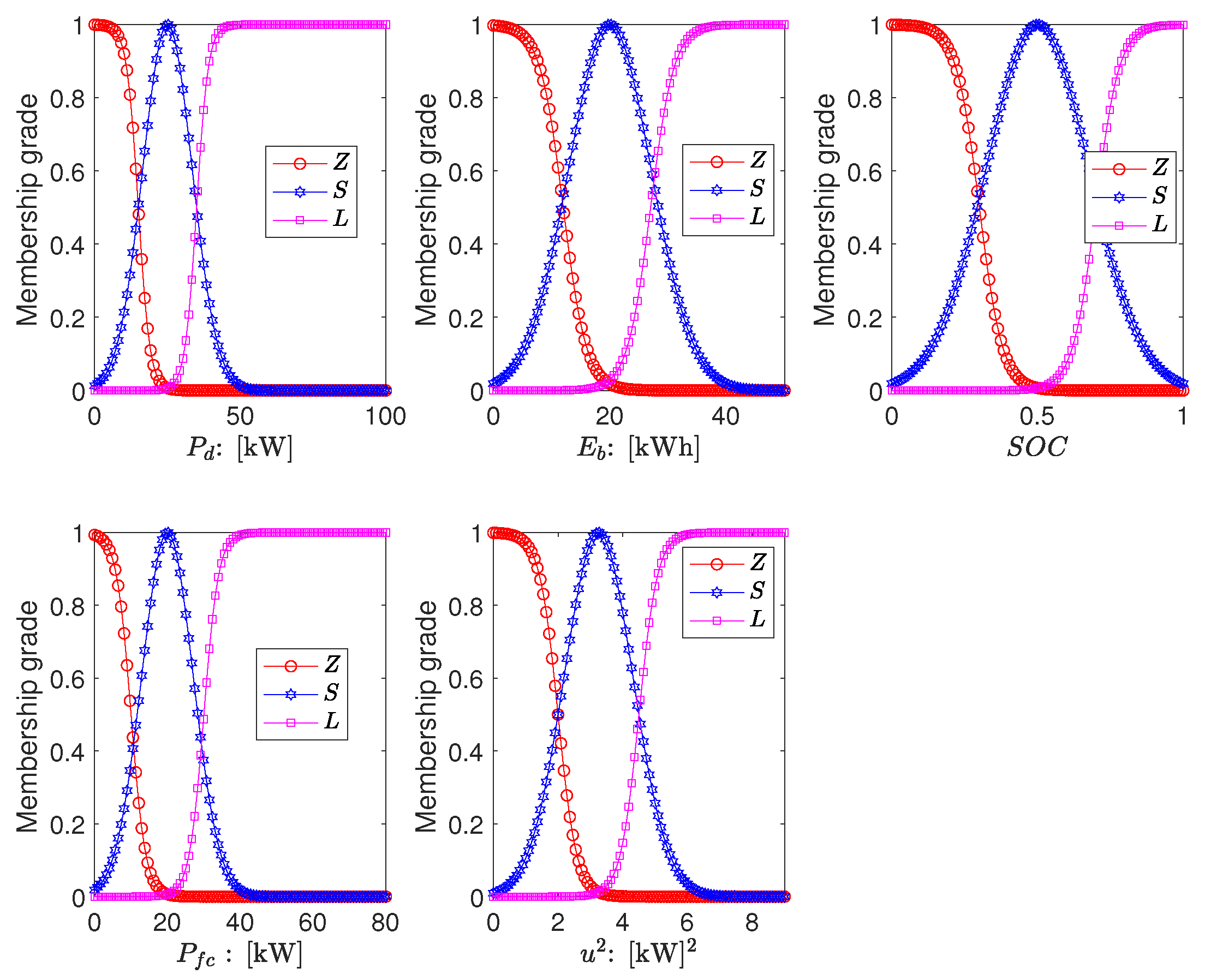
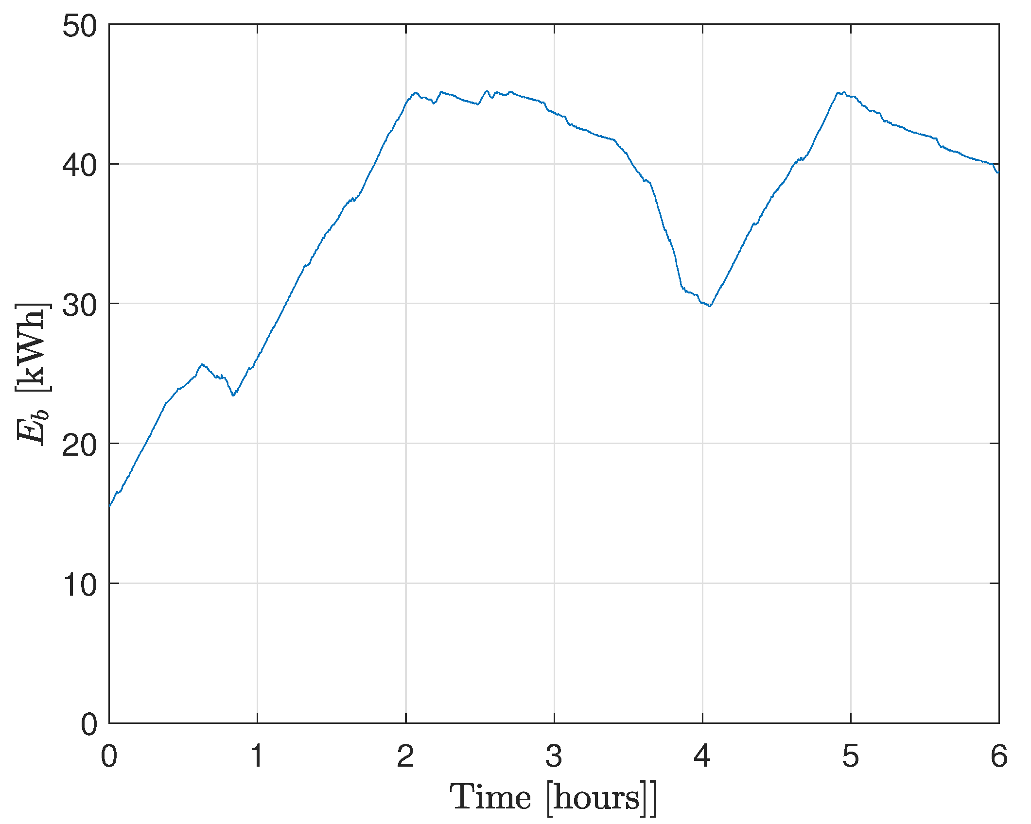
To implement the proposed scheme, the membership functions for all inputs of both MiFRENm and MiFRENs, as illustrated in Figure 5, are designed in accordance with the constraints specified in Equation (6) and Table 2. It is worth noting that, for comparative purposes, the battery power P b ( k ) [kW] is reformulated as the stored energy within the battery, E b ( k ) [kWh], defined as
E b ( k ) = E b ( k 1 ) + P b ( k ) T s 3 , 600 .
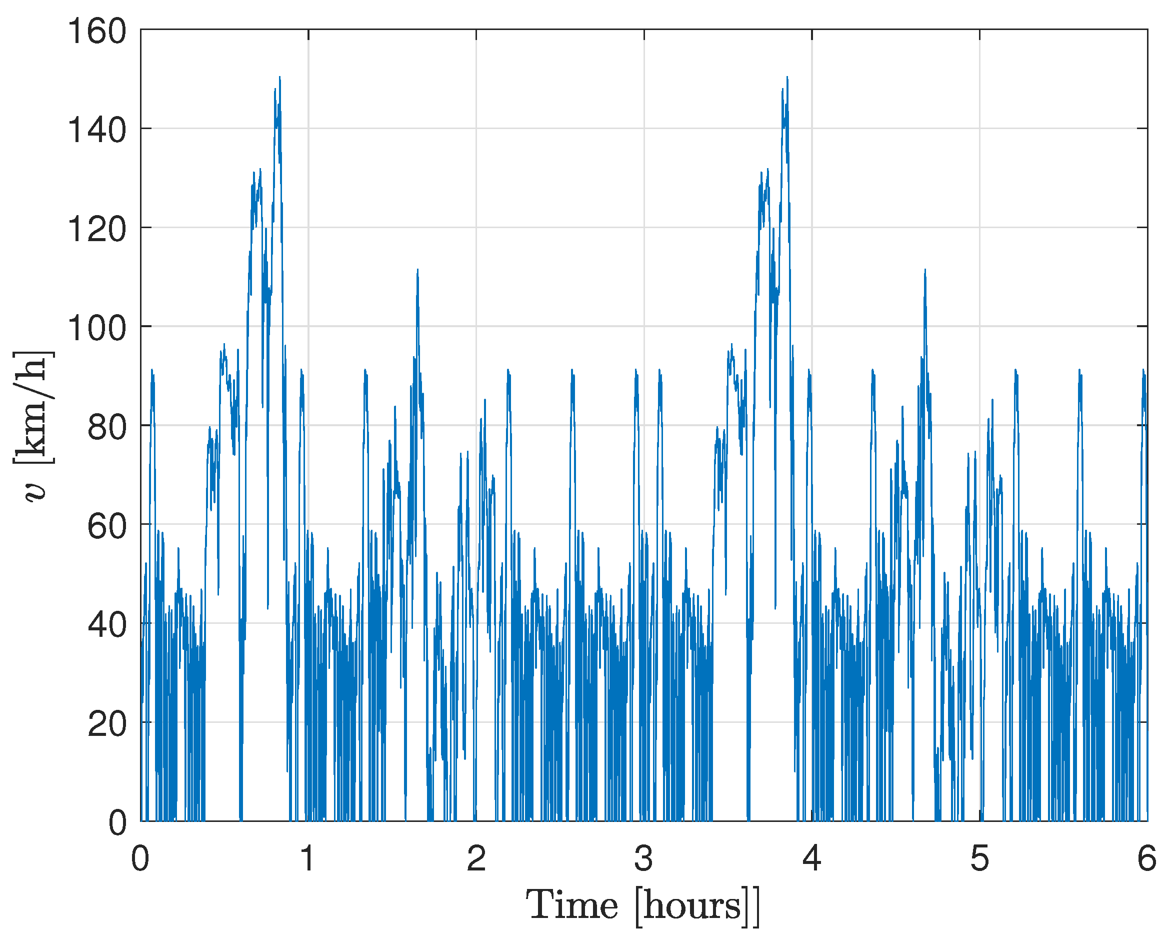
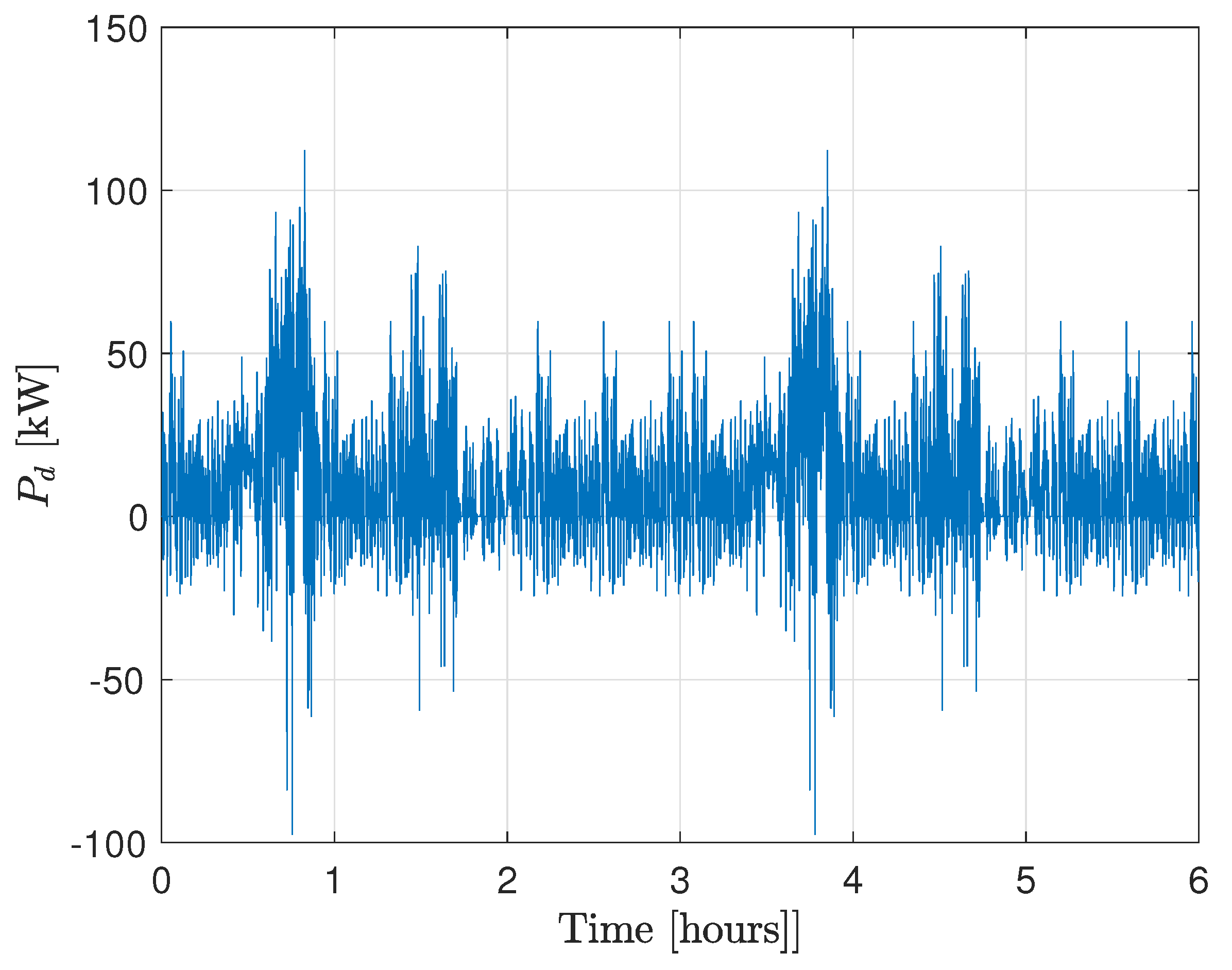
The velocity trajectory shown in Figure 6 is constructed by sequentially combining standard driving cycles, including UDDS, HWFET, ArtMw150, FTP, ArtRoad, and WLTP2 [2,12,20,25]. These datasets are recorded with a sampling interval of 1 [s]; thus, the sampling time is defined as T s = 1 [s]. Based on the selected velocity profiles and corresponding road conditions, the resulting power demand trajectory P d ( k ) is computed and illustrated in Figure 7.
To employ the proposed scheme, the initial battery energy is set to E b ( 1 ) = 15.5 [kWh], which determines the initial value of S O C as
S O C ( 1 ) = E b ( 1 ) E 0 = 15.5 50 = 0.31 .
Subsequently, S O C r ( k + 1 ) is generated in real time according to the relation in (12), with δ S O C = 0.95 . Therefore, the learning laws of MiFRENm, given in Equations (30) and (31), and MiFRENs, given in Equation (48), are employed with learning rates γ e = 0.5 and γ λ = 0.5 , respectively.
Under the proposed controller, the time-varying behavior of the fuel cell power P f c ( k ) is shown in Figure 8, with the corresponding control effort u ( k ) , represented as Δ P f c ( k ) , illustrated in Figure 9. The results indicate that the controller successfully maintains the fuel cell power output at a nearly constant level for the majority of the operation period, while strictly adhering to the lower and upper power constraints defined in Table 2. The battery energy evolution E b ( k ) , shown in Figure 10, reveals that despite starting from a low initial energy level, the controller is able to sustain an adequate battery charge throughout the drive cycle. Furthermore, Figure 11 compares the actual state of charge S O C ( k ) with the reference trajectory S O C r ( k ) , demonstrating accurate tracking performance under varying operational conditions. To highlight the adaptive behavior of the proposed networks, Figure 12 illustrates the evolution of the time-varying learning rates η e ( k ) and η λ ( k ) , which govern the online adaptation of MiFRENm and MiFRENs, respectively. Nonetheless, it is worth remarking that the fluctuations observed in the reference state of charge S O C r ( k ) are closely associated with variations in the co-state learning rate η λ ( k ) , as illustrated in Figure 12. This correlation highlights the effectiveness of the proposed scheme, wherein the adaptive learning mechanism enables the controller to accurately manage the behavior of the actual S O C ( k ) —particularly under high charge conditions. These learning rates dynamically respond to system variations, contributing to the robustness and real-time adaptability of the control strategy.

4.2. Comparative Results

4.2.1. Comparative Controller A

The comparative controller A is developed based on the concept of maintaining S O C ( k ) approximately constant, following the algorithm proposed in [25]. All design parameters are selected in accordance with Table 6 of [25], except that the minibatch size is increased to 256, as suggested by the numerical formulation in [12], to enhance performance. This adjustment is justified by the extended validation period in this work, which spans 6 h compared to only 0.67 h in [25].
In this case, the fuel cell power output P f c ( k ) under Controller A is depicted in Figure 13. In comparison with the results obtained using the proposed controller (Figure 8), it is apparent that Controller A induces more pronounced high-frequency fluctuations in P f c ( k ) . This behavior may impose additional stress on the fuel cell system and could potentially reduce its operational lifespan. Figure 14 presents the battery energy trajectory E b ( k ) , indicating that the controller maintains the battery around its nominal energy level throughout the driving cycle. Additionally, Figure 15 shows the evolution of the state of charge S O C ( k ) , demonstrating that Controller A achieves its design objective of regulating S O C ( k ) near a constant value. Nonetheless, it is important to note that this approach may sacrifice smooth fuel cell operation in favor of maintaining a steady battery charge.

4.2.2. Comparative Controller B

To address the issue of high-frequency variations in P f c ( k ) , the soft actor–critic scheme developed in [2] is adopted as Controller B. All design parameters are chosen in accordance with Table 4 of [2], except for the discount factor, which is set to γ = 0.95 to optimize performance for the current validation case. It is important to note that this approach requires additional information, such as a thermal load model and a detailed description of the air conditioning system, which together allow for a well-defined formulation of P a u x ( k ) . However, in the context of this validation test, P a u x ( k ) is treated as an unknown disturbance. Consequently, the learning algorithm proposed in [20] is employed to train both the actor and critic networks, with the learning rates reselected to 0.001.
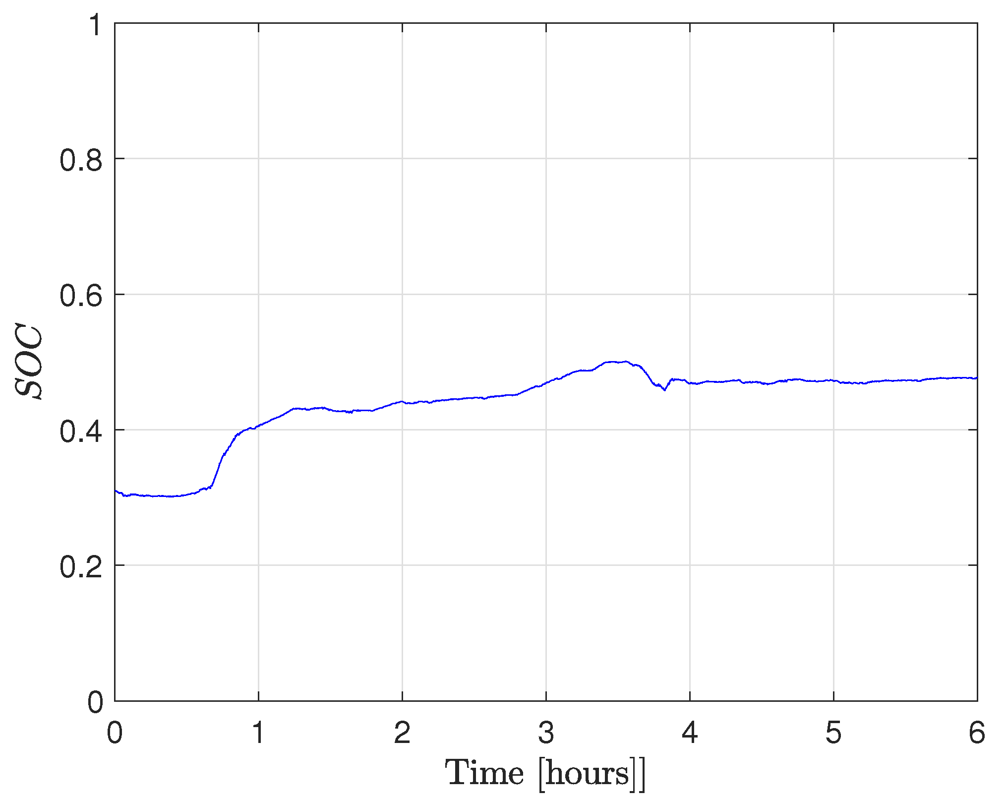
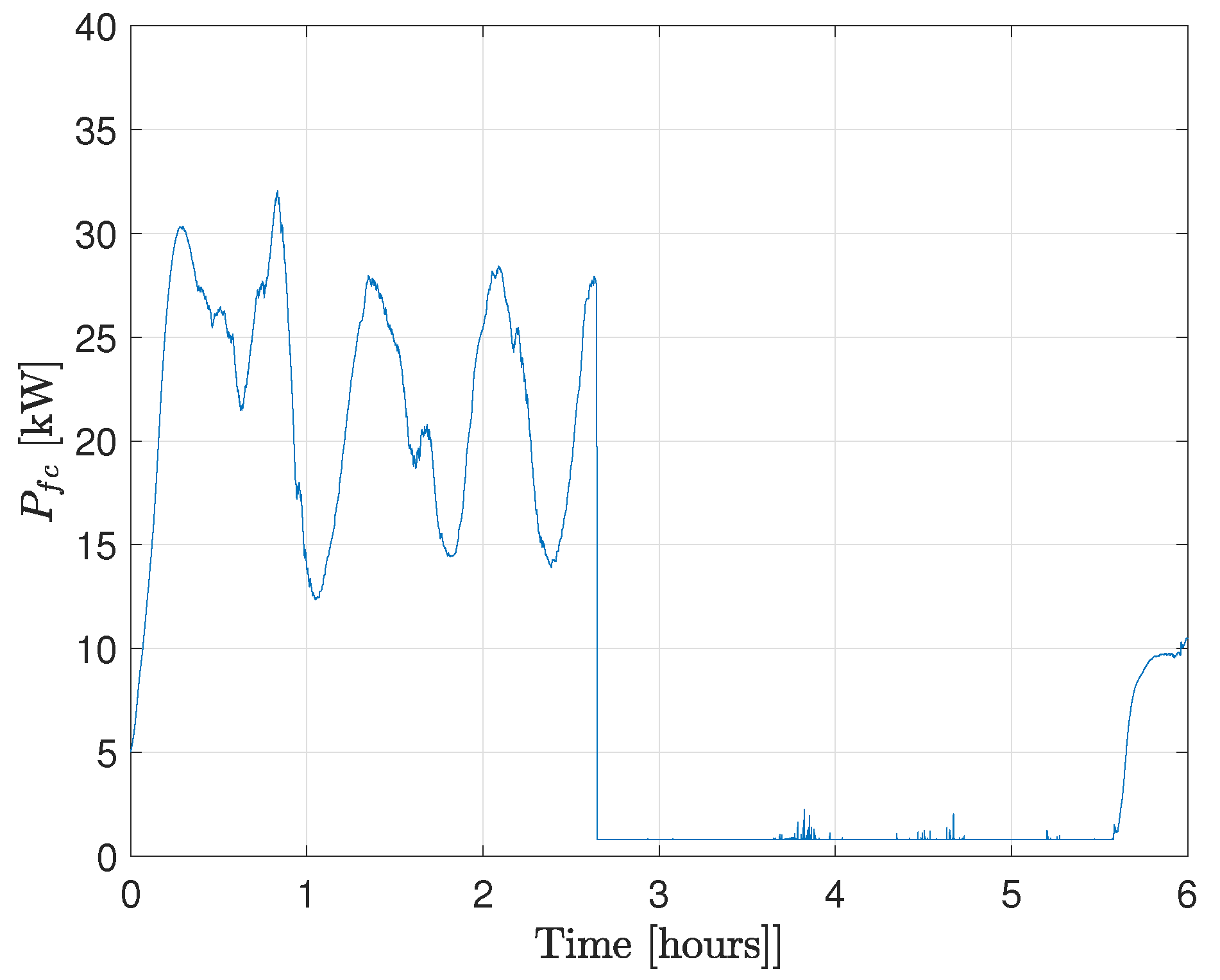
As a result, the power output P f c ( k ) generated by Controller B is illustrated in Figure 16. In comparison with Controller A, it is evident that the high-frequency components have been significantly suppressed, indicating smoother fuel cell operation. However, some transient variations are observed during the initial hour of operation, likely due to the adaptation period of the learning-based controller. Furthermore, Figure 17 presents the evolution of S O C ( k ) under Controller B. While the state of charge is successfully maintained within the specified operational limits, the S O C ( k ) trajectory exhibits slightly larger oscillations compared to those obtained with the proposed controller and Controller A.

5. Conclusions

This work has presented a data-driven energy management strategy for fuel cell and battery electric vehicles, formulated as a constrained optimal control problem. The proposed approach has integrated a co-state network with online learning to estimate the optimal control input in real time, eliminating the need for prior system modeling or complete operational datasets and avoiding dimensionality challenges common in many learning-based methods. Robustness has been achieved by treating unknown and time-varying disturbances—such as auxiliary power consumption, road slope variations, and passenger-related loads—as bounded system uncertainties. The controller has aimed to track a desired SOC trajectory while respecting all physical constraints and adapting effectively to changing operating conditions without requiring offline training or predictive models. Validation results obtained over a six-hour composite driving profile—comprising UDDS, HWFET, ArtMw150, FTP, ArtRoad, and WLTP2 cycles—have demonstrated the following:
  • Stable battery operation with SOC maintained within a practical range;
  • A significant reduction in high-frequency fluctuations of fuel cell power output compared to benchmark controllers;
  • Improved overall energy efficiency relative to constant SOC and soft actor–critic methods.
Comparative analysis against a constant SOC controller and a soft actor–critic algorithm has further confirmed the proposed scheme’s advantages in terms of stability, robustness to unknown disturbances, and real-time computational feasibility. Building upon the benefits of the online learning framework developed in this work, integration with traffic and route information—by leveraging vehicle-to-everything (V2X) and route-based forecasting—has been identified as a promising direction for future research to further enhance predictive capabilities and energy efficiency under real-world driving conditions.

Author Contributions

Conceptualization, C.T.; Methodology, S.K.K. and C.P.; Validation, C.T., A.D.M.-V. and B.S.; Formal analysis, S.K.K. and B.S.; Investigation, C.T., A.D.M.-V., S.K.K. and C.P.; Data curation, B.S.; Writing—original draft, C.T. and A.D.M.-V. All authors have read and agreed to the published version of the manuscript.

Funding

This research received no external funding.

Data Availability Statement

Data is contained within the article.

Conflicts of Interest

The authors declare no conflicts of interest.

References

  1. Sidharthan, V.P.; Kashyap, Y.; Kosmopoulos, P. Adaptive-Energy-Sharing-Based Energy Management Strategy of Hybrid Sources in Electric Vehicles. Energies 2023, 16, 1214. [Google Scholar] [CrossRef]
  2. Deng, L.; Li, S.; Tang, X.; Yang, K.; Lin, X. Battery thermal- and cabin comfort-aware collaborative energy management for plug-in fuel cell electric vehicles based on the soft actor–critic algorithm. Energy Convers. Manag. 2023, 283, 116889. [Google Scholar] [CrossRef]
  3. Chan, C.C. The State of the Art of Electric, Hybrid, and Fuel Cell Vehicles. Proc. IEEE 2007, 95, 704–718. [Google Scholar] [CrossRef]
  4. Gioffrè, D.; Manzolini, G.; Leva, S.; Jaboeuf, R.; Tosco, P.; Martelli, E. Quantifying the Economic Advantages of Energy Management Systems for Domestic Prosumers with Electric Vehicles. Energies 2025, 18, 1774. [Google Scholar] [CrossRef]
  5. Wang, C.; Liu, Y.; Zhang, Y.; Xi, L.; Yang, N.; Zhao, Z.; Lai, C.S.; Lai, L.L. Strategy for optimizing the bidirectional time-of-use electricity price in multi-microgrids coupled with multilevel games. Energy 2025, 323, 135731. [Google Scholar] [CrossRef]
  6. Maroufi, S.M.; Karrari, S.; Rajashekaraiah, K.; De Carne, G. Power Management of Hybrid Flywheel-Battery Energy Storage Systems Considering the State of Charge and Power Ramp Rate. IEEE Trans. Power Electron. 2025, 40, 9944–9956. [Google Scholar] [CrossRef]
  7. Nawaz, M.; Ahmed, J.; Abbas, G. Energy-efficient battery management system for healthcare devices. J. Energy Storage 2022, 51, 104358. [Google Scholar] [CrossRef]
  8. Uralde, J.; Barambones, O.; del Rio, A.; Calvo, I.; Artetxe, E. Rule-Based Operation Mode Control Strategy for the Energy Management of a Fuel Cell Electric Vehicle. Batteries 2024, 10, 214. [Google Scholar] [CrossRef]
  9. Li, Y.; Pu, Z.; Liu, P.; Qian, T.; Hu, Q.; Zhang, J.; Wang, Y. Efficient predictive control strategy for mitigating the overlap of EV charging demand and residential load based on distributed renewable energy. Renew. Energy 2025, 240, 122154. [Google Scholar] [CrossRef]
  10. Kim, D.J.; Kim, B.; Yoon, C.; Nguyen, N.D.; Lee, Y.I. Disturbance Observer-Based Model Predictive Voltage Control for Electric-Vehicle Charging Station in Distribution Networks. IEEE Trans. Smart Grid 2023, 14, 545–558. [Google Scholar] [CrossRef]
  11. Khan, B.; Ullah, Z.; Gruosso, G. Enhancing Grid Stability Through Physics-Informed Machine Learning Integrated-Model Predictive Control for Electric Vehicle Disturbance Management. World Electr. Veh. J. 2025, 16, 292. [Google Scholar] [CrossRef]
  12. Khan, K.; Samuilik, I.; Ali, A. A Mathematical Model for Dynamic Electric Vehicles: Analysis and Optimization. Mathematics 2024, 12, 224. [Google Scholar] [CrossRef]
  13. Previti, U.; Brusca, S.; Galvagno, A.; Famoso, F. Influence of Energy Management System Control Strategies on the Battery State of Health in Hybrid Electric Vehicles. Sustainability 2022, 14, 12411. [Google Scholar] [CrossRef]
  14. Meteab, W.K.; Alsultani, S.A.H.; Jurado, F. Energy Management of Microgrids with a Smart Charging Strategy for Electric Vehicles Using an Improved RUN Optimizer. Energies 2023, 16, 6038. [Google Scholar] [CrossRef]
  15. Shen, Y.; Li, Y.; Liu, D.; Wang, Y.; Sun, J.; Sun, S. Energy Management Strategy for Hybrid Energy Storage System based on Model Predictive Control. J. Electr. Eng. Technol. 2023, 18, 3265–3275. [Google Scholar] [CrossRef]
  16. Oksuztepe, E.; Yildirim, M. PEM fuel cell and supercapacitor hybrid power system for four in-wheel switched reluctance motors drive EV using geographic information system. Int. J. Hydrogen Energy 2024, 75, 74–87. [Google Scholar] [CrossRef]
  17. Gao, H.; Yin, B.; Pei, Y.; Gu, H.; Xu, S.; Dong, F. An energy management strategy for fuel cell hybrid electric vehicle based on a real-time model predictive control and pontryagin’s maximum principle. Int. J. Green Energy 2024, 21, 2640–2652. [Google Scholar] [CrossRef]
  18. Liu, W.; Yao, P.; Wu, Y.; Duan, L.; Li, H.; Peng, J. Imitation reinforcement learning energy management for electric vehicles with hybrid energy storage system. Appl. Energy 2025, 378, 124832. [Google Scholar] [CrossRef]
  19. Han, R.; He, H.; Wang, Y.; Wang, Y. Reinforcement Learning Based Energy Management Strategy for Fuel Cell Hybrid Electric Vehicles. Chin. J. Mech. Eng. 2025, 38, 66. [Google Scholar] [CrossRef]
  20. Guo, D.; Lei, G.; Zhao, H.; Yang, F.; Zhang, Q. The A3C Algorithm with Eligibility Traces of Energy Management for Plug-In Hybrid Electric Vehicles. IEEE Access 2025, 13, 92507–92518. [Google Scholar] [CrossRef]
  21. Liu, H.; You, C.; Han, L.; Yang, N.; Liu, B. Off-road hybrid electric vehicle energy management strategy using multi-agent soft actor–critic with collaborative-independent algorithm. Energy 2025, 328, 136463. [Google Scholar] [CrossRef]
  22. Wang, J.; Du, C.; Yan, F.; Duan, X.; Hua, M.; Xu, H.; Zhou, Q. Energy Management of a Plug-In Hybrid Electric Vehicle Using Bayesian Optimization and Soft Actor–Critic Algorithm. IEEE Trans. Transp. Electrif. 2025, 11, 912–921. [Google Scholar] [CrossRef]
  23. Sun, Z.; Guo, R.; Luo, M. Integrated energy-thermal management strategy for range extended electric vehicles based on soft actor–critic under low environment temperature. Energy 2025, 330, 136868. [Google Scholar] [CrossRef]
  24. Wang, C.; Zhang, J.; Wang, A.; Wang, Z.; Yang, N.; Zhao, Z.; Lai, C.S.; Lai, L.L. Prioritized sum-tree experience replay TD3 DRL-based online energy management of a residential microgrid. Appl. Energy 2024, 368, 123471. [Google Scholar] [CrossRef]
  25. Jia, C.; He, H.; Zhou, J.; Li, J.; Wei, Z.; Li, K. Learning-based model predictive energy management for fuel cell hybrid electric bus with health-aware control. Appl. Energy 2024, 355, 122228. [Google Scholar] [CrossRef]
  26. Cavus, M.; Dissanayake, D.; Bell, M. Next Generation of Electric Vehicles: AI-Driven Approaches for Predictive Maintenance and Battery Management. Energies 2025, 18, 1041. [Google Scholar] [CrossRef]
  27. Omakor, J.; Alzayed, M.; Chaoui, H. Particle Swarm-Optimized Fuzzy Logic Energy Management of Hybrid Energy Storage in Electric Vehicles. Energies 2024, 17, 2163. [Google Scholar] [CrossRef]
  28. Treesatayapun, C. Prescribed performance of discrete-time controller based on the dynamic equivalent data model. Appl. Math. Model. 2020, 78, 366–382. [Google Scholar] [CrossRef]
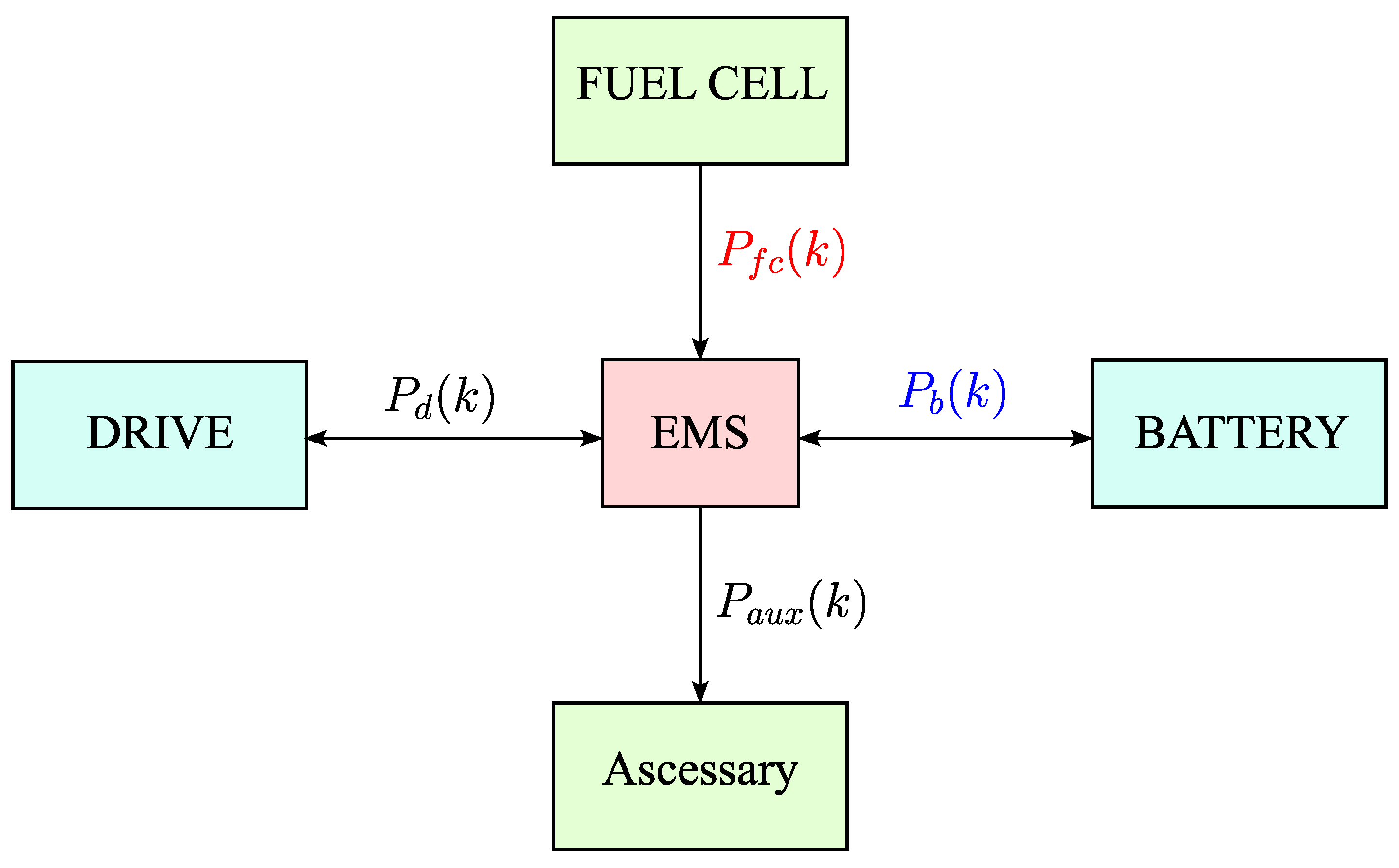
Figure 1. Power flow block diagram.
Energies 18 04062 g001
Figure 2. MiFRENm architecture: Model network.
Energies 18 04062 g002
Figure 3. MiFRENs architecture: Co-state network.
Energies 18 04062 g003
Figure 4. Control system block diagram.
Energies 18 04062 g004
Figure 5. Membership functions.
Energies 18 04062 g005
Figure 6. Velocity profile.
Energies 18 04062 g006
Figure 7. Demanding power: P d ( k ) .
Energies 18 04062 g007
Figure 8. Proposed controller: P f c ( k ) .
Energies 18 04062 g008
Figure 9. Proposed controller: u ( k ) or Δ P f c ( k ) .
Energies 18 04062 g009
Figure 10. Proposed controller: E b ( k ) .
Energies 18 04062 g010
Figure 11. Proposed controller: S O C ( k ) .
Energies 18 04062 g011
Figure 12. Proposed controller: η e ( k ) and η λ ( k ) .
Energies 18 04062 g012
Figure 13. Controller A: P f c ( k ) .
Energies 18 04062 g013
Figure 14. Controller A: E b ( k ) .
Energies 18 04062 g014
Figure 15. Controller A: S O C ( k ) .
Energies 18 04062 g015
Figure 16. Controller B: P f c ( k ) .
Energies 18 04062 g016
Figure 17. Controller B: S O C ( k ) .
Energies 18 04062 g017
Table 1. System parameters.
ParameterDescriptionValueUnitRemark
C d Aerodynamic drag coefficient0.3
A f Fronted area2.2508[ m 2 ]
ρ a Air density1.293[k/ m 3 ]
m 0 Curb weight2024[kg]
R i Rotational inertia coefficient1
R r Rolling resistance coefficient0.013
gGravity acceleration9.81[m/ s 2 ]
η e m Motor efficiency0.9
η m Mechanical drive efficiency0.9
η D C / A C Inverter efficiency0.95
η D C / D C Converter efficiency0.95
η b Coulombic efficiency0.98
E 0 Battery capacity50[kWh]
Table 2. Constraint parameters.
LimitValueUnitLimitValueUnit
P f c m i n 0.25[kW] P f c m a x 80[kW]
Δ P f c M 9[kW] P b M 50[kW]
S O C m i n 0.2Per Unit S O C m a x 0.9Per Unit
P d G e n 80[kW] P d D r v 100[kW]
P a u x m i n 0.5[kW] P a u x m a x 20[kW]
I b M 50[A]
Disclaimer/Publisher’s Note: The statements, opinions and data contained in all publications are solely those of the individual author(s) and contributor(s) and not of MDPI and/or the editor(s). MDPI and/or the editor(s) disclaim responsibility for any injury to people or property resulting from any ideas, methods, instructions or products referred to in the content.