Research and Application of Low-Velocity Nonlinear Seepage Model for Unconventional Mixed Tight Reservoir

Abstract

Due to factors such as low porosity and permeability, thin sand body thickness, and strong interlayer heterogeneity, the fluid flow in the tight reservoir (beach-bar sandstone reservoir) exhibits obvious nonlinear seepage characteristics. Considering the time-varying physical parameters of different types of sand bodies, a nonlinear seepage coefficient is derived based on permeability and capillary force, and a low-velocity nonlinear seepage model for beach bar sand reservoirs is established. Based on core displacement experiments of different types of sand bodies, the low-velocity nonlinear seepage coefficient was fitted and numerical simulation of low-velocity nonlinear seepage in beach-bar sandstone reservoirs was carried out. The research results show that the displacement pressure and flow rate of low-permeability tight reservoirs exhibit a significant nonlinear relationship. The lower the permeability and the smaller the displacement pressure, the more significant the nonlinear seepage characteristics. Compared to the bar sand reservoir, the water injection pressure in the tight reservoir of the beach sand is higher. In the nonlinear seepage model, the bottom hole pressure of the water injection well increases by 10.56% compared to the linear model, indicating that water injection is more difficult in the beach sand reservoir. Compared to matrix type beach sand reservoirs, natural fractures can effectively reduce the impact of fluid nonlinear seepage characteristics on the injection and production process of beach sand reservoirs. Based on the nonlinear seepage characteristics, the beach-bar sandstone reservoir can be divided into four flow zones during the injection production process, including linear seepage zone, nonlinear seepage zone, non-flow zone affected by pressure, and non-flow zone not affected by pressure. The research results can effectively guide the development of beach-bar sandstone reservoirs, reduce the impact of low-speed nonlinear seepage, and enhance oil recovery.

1. Introduction

With the development of oil and gas exploration and development technology, oil and gas development has shifted from conventional reservoirs to low-permeability and tight unconventional reservoirs, with deeper burial depth, higher temperature and pressure, and poorer physical properties [1,2]. Beach-bar sandstone reservoirs are currently one of the hotspots in unconventional oil and gas development, among which beach sand is a typical low-permeability tight reservoir. In water drive reservoirs, vertical heterogeneity can significantly affect the stability of the displacement front, leading to premature water breakthrough, reduced vertical sweep efficiency, and final recovery rate [3]. Due to factors such as low porosity and permeability, thin sand body thickness, and strong interlayer heterogeneity, it is difficult to reservoir stimulation [4,5]. Due to the complex seepage environment and narrow pore throat, the fluid flow in low-permeability tight reservoirs relies on narrow channels, resulting in high seepage resistance [6,7,8]. In addition, there are significant forces at the solid–liquid and liquid–liquid interfaces. Therefore, in addition to overcoming viscous resistance, fluid flow in porous media must also overcome the interaction between the solid–liquid interfacial tension in the oil–water boundary layer. When the displacement pressure is greater than the threshold value, the fluid will flow, that is, there is a starting pressure for fluid flow. On the other hand, the physical properties of low-permeability tight reservoirs are greatly affected by changes in overlying pressure, resulting in changes in fluid flow patterns that deviate from the classic Darcy flow pattern, exhibiting low-velocity nonlinear seepage characteristics in tight reservoirs [9,10,11]. At present, conventional commercial software (Eclipse, CMG, etc.) for reservoir numerical simulation at home and abroad are based on the Darcy flow model, which is mainly applied to medium and high permeability oil and gas reservoirs. Therefore, it is necessary to study the low-velocity non-Darcy flow model and flow law for low permeability tight reservoirs [12,13,14].

Since the 1990s, domestic and foreign scholars have studied the low-velocity nonlinear seepage phenomenon in low-permeability tight reservoirs through experimental testing and numerical simulation methods [15,16,17,18]. Based on the research results, three conclusions have been drawn: (1) Scholars generally recognize that the flow of fluids in low-permeability tight reservoirs is low-speed non-Darcy seepage, and Darcy seepage models exaggerate the reservoir’s seepage capacity. (2) The quasi starting pressure gradient model proposed by some scholars cannot characterize the low-speed nonlinear seepage stage, indicating an increase in reservoir seepage resistance, resulting in significant errors in the prediction results of numerical simulation software using the quasi starting pressure gradient model. (3) Some scholars have proposed a numerical simulation method for variable permeability, which can accurately describe non-Darcy flow in porous media of low permeability and tight reservoirs. However, a continuous and smooth permeability state equation has not been provided, and existing numerical simulation software for variable permeability has not been able to provide the changes in pressure gradient field and permeability field [19,20,21]. Therefore, the numerical simulation method for variable permeability has not been widely applied.

In summary, the current low-velocity nonlinear seepage models mainly include segmented models, continuous nonlinear seepage models, and quasi starting pressure gradient models [22,23,24,25]. As shown in Figure 1, most existing nonlinear seepage models adopt fixed nonlinear seepage coefficients. According to the actual situation of the formation, with the progress of production, the formation pressure and reservoir properties are constantly changing, so the form of underground nonlinear seepage is also constantly changing with the progress of production [26,27,28]. Therefore, based on the research results, this paper deduces a continuous nonlinear seepage equation considering the influence of time-varying physical properties (permeability, pressure gradient), and establishes a low-velocity nonlinear seepage model for tight beach-bar sandstone reservoirs by fitting the nonlinear seepage coefficient based on permeability and capillary force.

2. Nonlinear Seepage Mathematical Model

Based on the capillary model, combined with the boundary layer theory, and considering the time-varying influence of reservoir physical properties, a continuous nonlinear seepage model is established. The assumption of the oil–water two-phase flow model in tight oil reservoirs is as follows: (1) considering the two-phase flow of oil and water in the reservoir, the fluid is incompressible; (2) initial yield stress τ₀ exists in fluid flow; (3) fluids move laminar in capillaries.

In the capillary model, the main driving force of fluid flow is the flow pressure difference ΔPπr²; the flow resistance is 2πrLτ. When stable seepage occurs in a capillary model, there are

$$\Delta p\pi r^2=2\pi rL\tau$$

(1)

where ΔP is the flow pressure difference between the head and tail ends of the capillary (Pa), R is the capillary radius (m), L is the capillary length (m), and τ is the fluid yield stress (Pa).

The constitutive equation of fluid flow yield stress is as follows:

$$\tau ={\tau }_0-\mu {\displaystyle \frac{\mathrm{d}v}{\mathrm{d}r}}$$

(2)

where τ₀ is the initial yield stress of the fluid (Pa), μ is the fluid viscosity (Pa·s), and ν is the flow velocity (m/s).

Based on the above two equations, it can be obtained that

$${\displaystyle \frac{\mathrm{d}v}{\mathrm{d}r}}={\displaystyle \frac{\Delta p}{2\mu L}}r+{\displaystyle \frac{{\tau }_0}{\mu }}$$

(3)

By integrating the above equation, it can be obtained that

$$v={\displaystyle \frac{\Delta p}{4\mu L}}[{(r_0-\delta )}^2-r^2]+{\displaystyle \frac{{\tau }_0}{\mu }}[r-(r_0-\delta )]$$

(4)

where r₀ is the initial capillary radius (m), and δ is the thickness of the fluid boundary layer in the capillary (m).

Where the fluid density is 1000 kg/m³, the viscosity is 1.5 mPa·s, the pore radius is 0.1 μm, the maximum flow velocity under the initial production pressure difference is 1.2 m/s, and the calculated Reynolds number Re is 2.5. If the Reynolds number is much less than 2300, it is considered laminar flow. The truncation error of high-order terms in the boundary layer is quantified by Taylor residual terms. The first-order main derivative term in the boundary layer term is negligible, and the order of high-order terms is less than 10⁻⁸.

The capillary flow rate is obtained as follows:

$$q={\displaystyle \frac{\pi r_0^4}{8\mu }}\nabla p{(1-{\displaystyle \frac{\delta }{r_0}})}^4[1-{\displaystyle \frac{8{\tau }_0}{3r_0(1-\frac{\delta }{r_0})\nabla p}}]$$

(5)

where q is the flow rate in the capillary tube (m³/s), and $\nabla p$ is the pressure gradient (Pa/m).

On the basis of the Kozeny model, the reservoir rock is regarded as a capillary bundle model with n capillaries, and the fluid passes vertically through the rock with an area of A, with a flow rate of

$$Q=nA{\displaystyle \frac{\pi r_0^4}{8\mu }}\nabla p{(1-{\displaystyle \frac{\delta }{r_0}})}^4[1-{\displaystyle \frac{8{\tau }_0}{3r_0(1-\frac{\delta }{r_0})\nabla p}}]$$

(6)

Based on the capillary model, its porosity and permeability are

$$\left\{\begin{array}{l}\varphi =n\pi r_0^2\\ K={\displaystyle \frac{\varphi r_0^2}{8}}\end{array}\right.$$

(7)

By handling the above two formulas, it can be obtained that

$$Q={\displaystyle \frac{K}{\mu }}A\nabla p{(1-{\displaystyle \frac{\delta }{r_0}})}^4[1-{\displaystyle \frac{8{\tau }_0}{3r_0(1-\frac{\delta }{r_0})\nabla p}}]$$

(8)

Based on the analysis of relevant experimental data, it can be considered that the thickness of the fluid boundary layer is negatively correlated with the pressure gradient in the capillary. The relevant assumptions of this model are as follows:

$$\left\{\begin{array}{l}a=\nabla p{\displaystyle \frac{\delta }{r_0}}\\ b={\displaystyle \frac{8{\tau }_0}{3r_0}}\end{array}\right.$$

(9)

By integrating the above equation, it can be obtained that

$$\begin{array}{l}Q={\displaystyle \frac{K}{\mu }}A\nabla p\left\{1-{\displaystyle \frac{4a+b}{\nabla p-a}}+{\displaystyle \frac{10a^2+4ab}{\nabla p\left(\nabla p-a\right)}}-\left[{\displaystyle \frac{4a^3}{{\left(\nabla p\right)}^3}}+{\displaystyle \frac{6a^{2}b+6a^3}{{\left(\nabla p\right)}^2\left(\nabla p-a\right)}}\right]+\right.\\ \left.\begin{array}{cc}& \begin{array}{cccc}& & & \end{array}\end{array}\left[{\displaystyle \frac{a^4}{{\left(\nabla p\right)}^4}}+{\displaystyle \frac{4a^{3}b}{{\left(\nabla p\right)}^3\left(\nabla p-a\right)}}\right]-{\displaystyle \frac{a^{4}b}{{\left(\nabla p\right)}^4\left(\nabla p-a\right)}}\right\}\end{array}$$

(10)

Due to the presence of

$$\left\{\begin{array}{l}{\displaystyle \frac{a}{\nabla p}}={\displaystyle \frac{\delta }{r_0}}<1\\ {\displaystyle \frac{b}{\nabla p-a}}={\displaystyle \frac{8{\tau }_0}{3r_0\left(1-\frac{\delta }{r_0}\right)\nabla p}}<1\end{array}\right.$$

(11)

Therefore, higher-order terms smaller than 1 in Equation (11) can be ignored, and Equation (11) can be simplified as follows:

$$Q={\displaystyle \frac{K}{\mu }}A\nabla p\left[1-{\displaystyle \frac{4a+b}{\nabla p-a}}+{\displaystyle \frac{10a^2+4ab}{\nabla p\left(\nabla p-a\right)}}\right]$$

(12)

In capillary flow, when the pressure gradient is $\nabla p=0$, there must be a flow rate of Q = 0. By incorporating the above formula, the coefficient term 10a² + 4ab = 0 can be obtained, which can simplify the above formula:

$$Q={\displaystyle \frac{K}{\mu }}A\left[1-{\displaystyle \frac{4a+b}{\nabla p-a}}\right]\nabla p$$

(13)

Assuming the coefficient terms 4a + b = c₁ and a = c₂ in the above formula, the formula can be simplified as follows:

$$Q={\displaystyle \frac{K}{\mu }}A\left[1-{\displaystyle \frac{c_1}{\nabla p-c_2}}\right]\nabla p$$

(14)

Due to the small pore throat and low oil/water flow rate of low-permeability tight reservoir, considering the influence of the fluid boundary layer and fluid yield stress, fluid flow in the tight reservoir has low-velocity nonlinear characteristics. The coefficients c₁ and c₂ in Equation (11) are characteristic parameters reflecting low-velocity nonlinear seepage, which can be obtained through experiments. When the pressure gradient is $\nabla p<c_1+c_2$, the fluid flow rate is 0, indicating the presence of a starting pressure gradient of $c_1+c_2$. Equation (14) can also be transformed into a Darcy flow model and a quasi starting pressure gradient model:

$$Q=\left\{\begin{array}{l}{\displaystyle \frac{K}{\mu }}A\nabla p\hspace{1em}\hspace{1em}\hspace{1em}\hspace{1em}, c_1=0\\ {\displaystyle \frac{K}{\mu }}A\left(1-{\displaystyle \frac{c_1}{\nabla p}}\right)\nabla p\hspace{1em}, c_2=0\end{array}\right.$$

(15)

3. Experimental Study on Nonlinear Seepage Flow

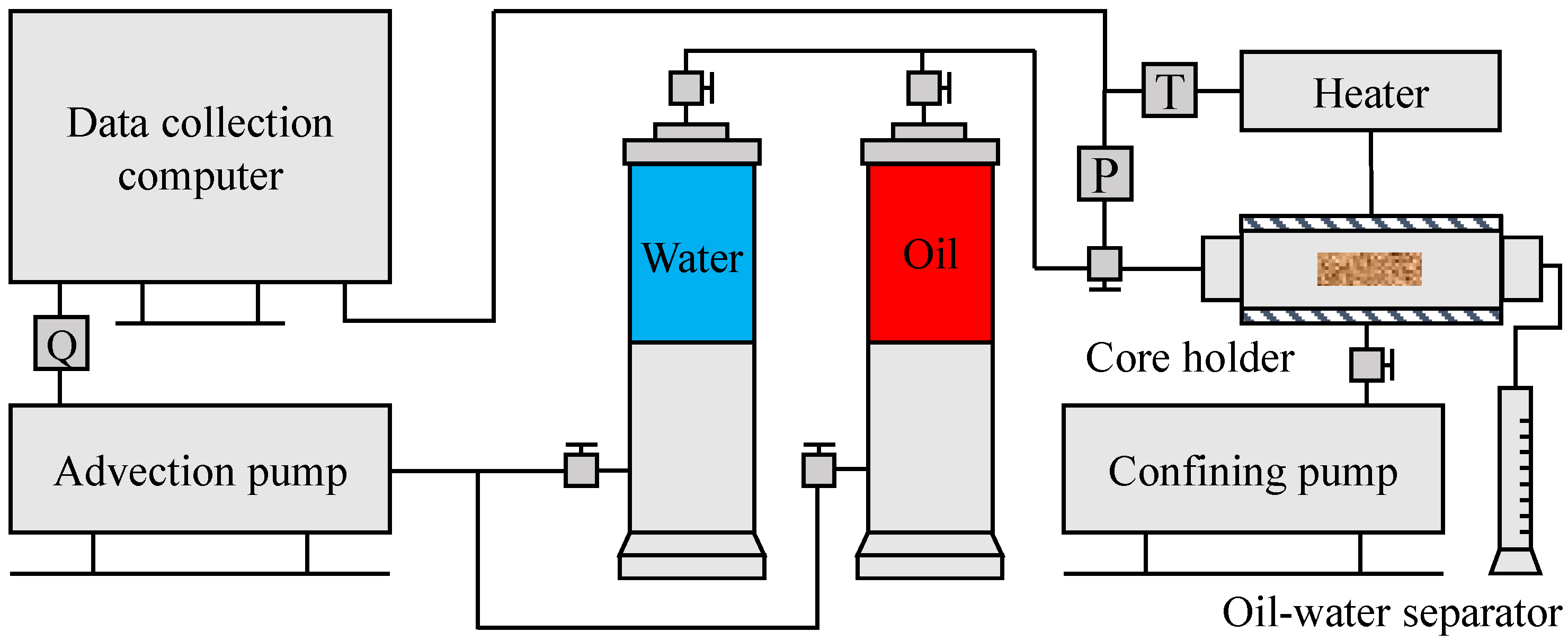
3.1. Experimental Methods

The nonlinear seepage characteristics of tight reservoirs are directly related to reservoir permeability. To obtain the nonlinear seepage coefficients c₁ and c₂ in the model, displacement experiments were designed for cores with different permeability. The experimental displacement medium uses standard formation water with a viscosity of 1 mPa·s to simulate formation fluid. The experimental device is shown in Figure 2. This paper selects 10 standard cores with different permeability for displacement experiments and records the displacement flow rate under different displacement pressure conditions. The experimental plan is shown in

Table 1. Displacement experiment plan.

Core Number	Core Diameter (cm)	Core Length (cm)	Core Permeability (mD)	Core Porosity (%)	K·A·μ−1 (cm4·MPa−1·s−1)
1—4	2.514	4.938	0.074	2.747	0.004
1—6	2.512	4.742	0.134	3.832	0.007
2—4	2.506	4.980	0.572	5.149	0.028
2—6	2.508	4.928	0.488	4.788	0.024
3—4	2.506	4.952	1.470	6.349	0.072
3—5	2.506	5.004	1.400	6.348	0.069
4—4	2.506	4.996	4.390	8.262	0.216
4—6	2.508	4.904	3.940	7.834	0.195
5—5	2.504	4.932	7.100	8.297	0.349
5—6	2.504	4.976	7.590	8.195	0.374

. To increase the accuracy of the experimental results, the following key measures were taken: (1) The rock cores were strictly cleaned and stabilized before testing. (2) Apply pressure gradients in descending order and maintain flow at each gradient point until the flow rate stabilizes before recording data. (3) The set maximum pressure gradient is much lower than the critical value estimated to cause significant structural changes.

During the experiment, the starting pressure of the core is very small and can be almost ignored. Therefore, Equation (14) is simplified as

$$Q={\displaystyle \frac{K}{\mu }}A\left[1-{\displaystyle \frac{m}{\nabla p+m}}\right]\nabla p$$

(16)

Define m in Equation (16) as the low-velocity nonlinear seepage coefficient, whose value characterizes the strength of the low-velocity nonlinear characteristics, that is, the larger the m, the more significant the nonlinear characteristics of the fluid during low-velocity flow in the rock core. Based on the pressure and flow data obtained from 10 different permeability core displacement experiments, as shown in Figure 3 and

Table 2. Displacement experiment results.

	Core Number	1—4	1—6	2—4	2—6	3—4	3—5	4—4	4—6	5—5	5—6
Pressure Gradient
0.02 MPa/cm		1.0 × 10−5	2.0 × 10−5	1.7 × 10−4	1.3 × 10−4	0.001	0.001	0.010	0.002	0.005	0.005
0.05 MPa/cm		5.0 × 10−5	1.1 × 10−4	0.001	0.001	0.002	0.002	0.033	0.007	0.015	0.016
0.1 MPa/cm		1.5 × 10−4	3.2 × 10−4	0.002	0.002	0.005	0.006	0.074	0.016	0.032	0.034
0.2 MPa/cm		4.2 × 10−4	0.001	0.004	0.004	0.014	0.012	0.169	0.036	0.068	0.073
0.3 MPa/cm		0.001	0.002	0.007	0.006	0.021	0.020	0.241	0.055	0.110	0.100
0.4 MPa/cm		0.001	0.002	0.011	0.008	0.026	0.026	0.340	0.075	0.131	0.153
0.5 MPa/cm		0.001	0.003	0.012	0.012	0.034	0.032	0.410	0.092	0.180	0.181
0.6 MPa/cm		0.002	0.003	0.015	0.012	0.039	0.040	0.513	0.118	0.201	0.226

, the m coefficient was fitted through a calculation program, and the fitting degree was greater than 0.95, indicating a high fitting degree, as shown in

Table 3. Low-velocity nonlinear seepage coefficient m.

Core Number	1—4	1—6	2—4	2—6	3—4	3—5	4—4	4—6	5—5	5—6
Permeability (mD)	0.074	0.134	0.572	0.488	1.470	1.400	4.390	3.940	7.100	7.590
Coefficient m	0.143	0.106	0.041	0.048	0.026	0.032	0.014	0.018	0.009	0.008
Fitting degree R	0.994	0.996	0.992	0.979	0.985	0.992	0.997	0.991	0.983	0.998

. The smaller the permeability is, the greater the m coefficient is, due to the influence of the fluid boundary layer and fluid yield stress in the pores, and the fluid flow shows significant non-Darcy characteristics. When the pressure gradient is less than 0.1 MPa/cm, there is a significant deviation from the linear relationship between pressure and velocity, resulting in strong nonlinear characteristics.

Based on the above analysis, the low speed nonlinear seepage coefficient m is fitted to an expression for permeability. The equation has a high degree of fitting, with a fitting degree R of 0.965. The equation is as follows:

$$m=0.032K^{-0.595}$$

(17)

By introducing m into the low-speed nonlinear seepage Equation (16), it can be obtained that

$$Q={\displaystyle \frac{K}{\mu }}A\left[1-{\displaystyle \frac{0.032K^{-0.595}}{\nabla p+0.032K^{-0.595}}}\right]\nabla p$$

(18)

Equation (18) can be used to establish a low-velocity nonlinear seepage model considering time-varying parameters of reservoir physical properties, which can more truly reflect the underground seepage process of tight reservoirs. Three groups of core samples (0.15–7.59 mD) that did not participate in the fitting test showed that the prediction error of the starting pressure gradient and nonlinear coefficient was less than 4.3%.

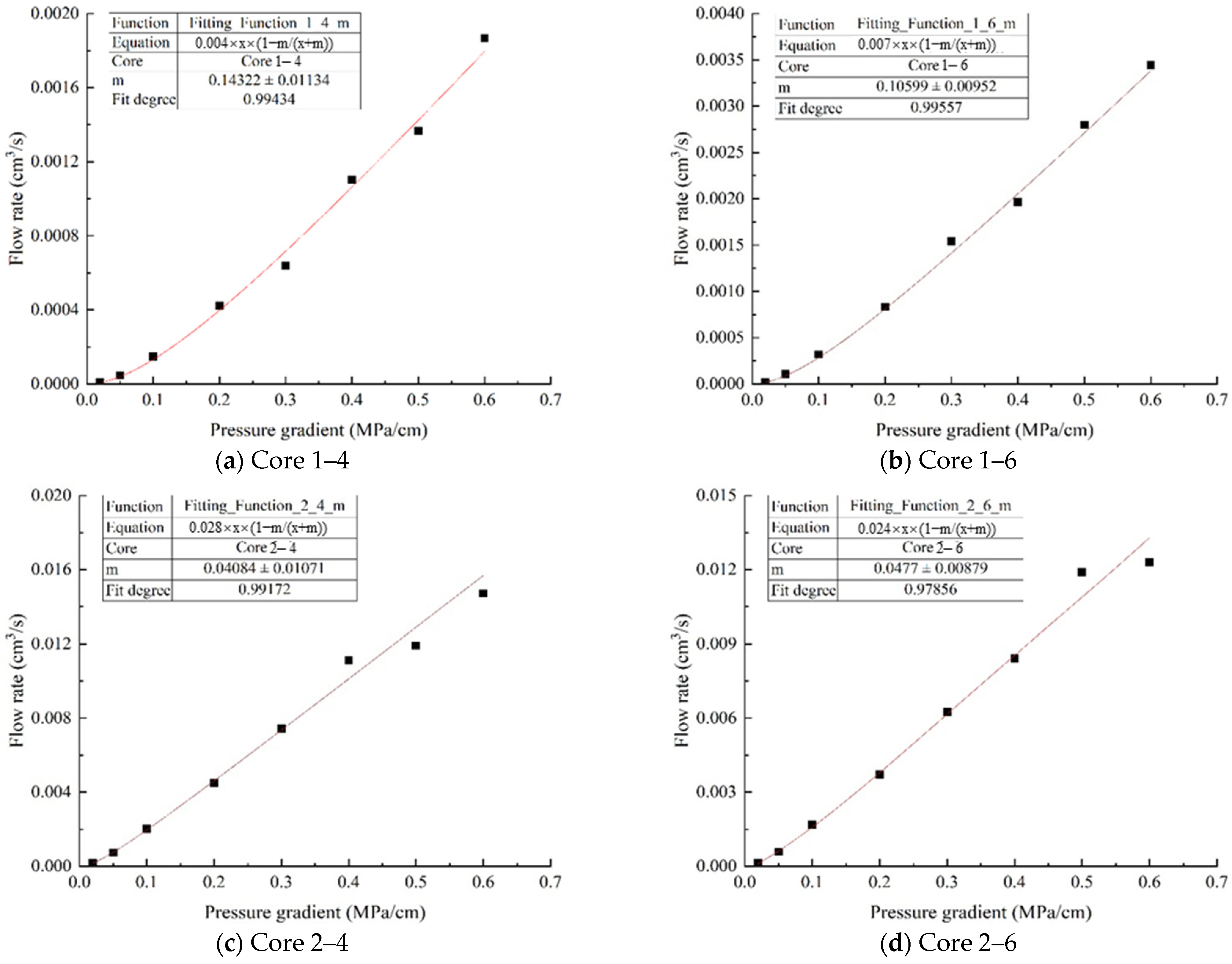
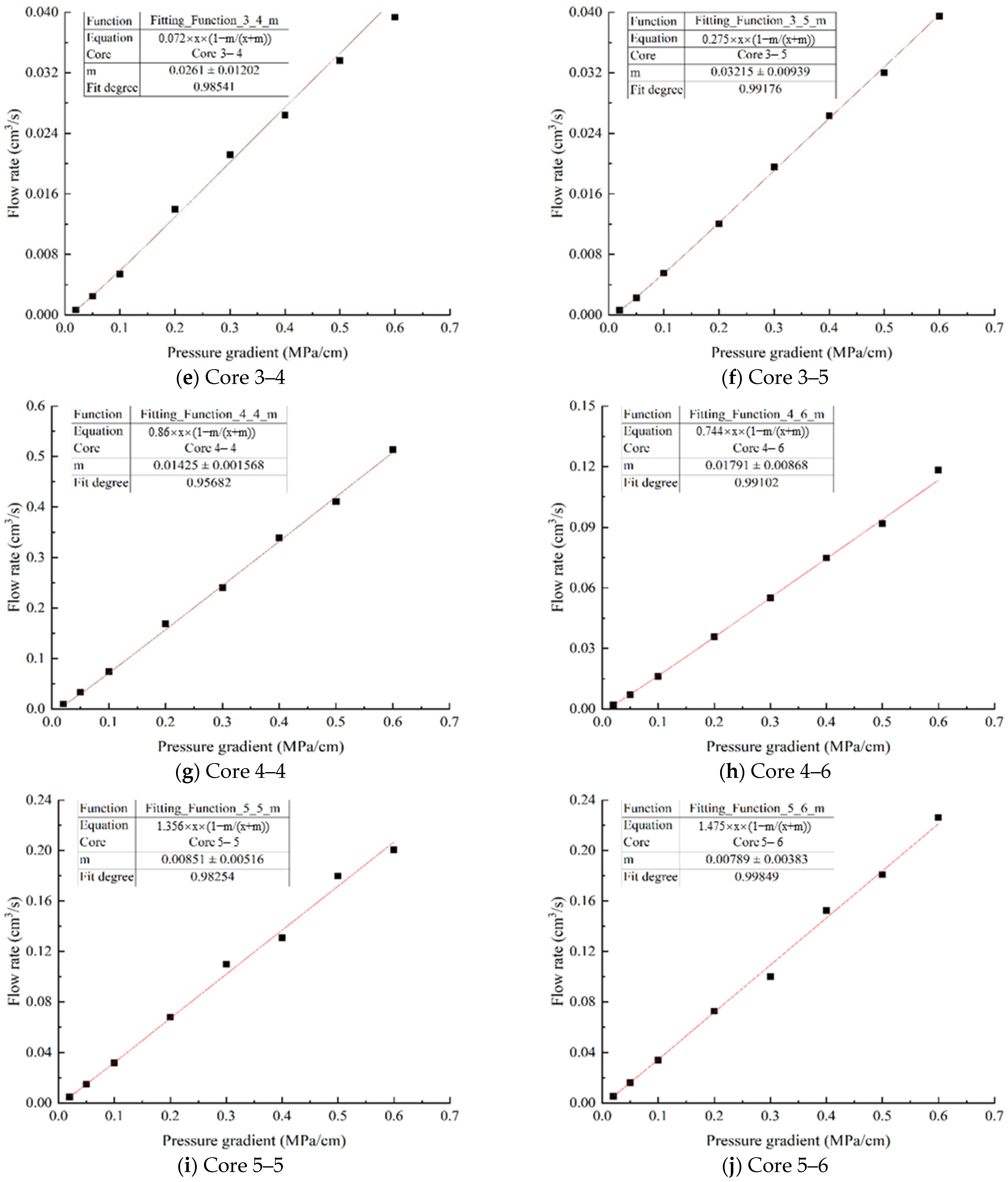
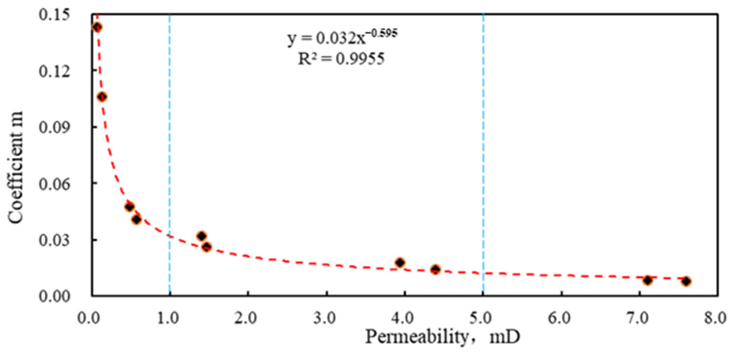
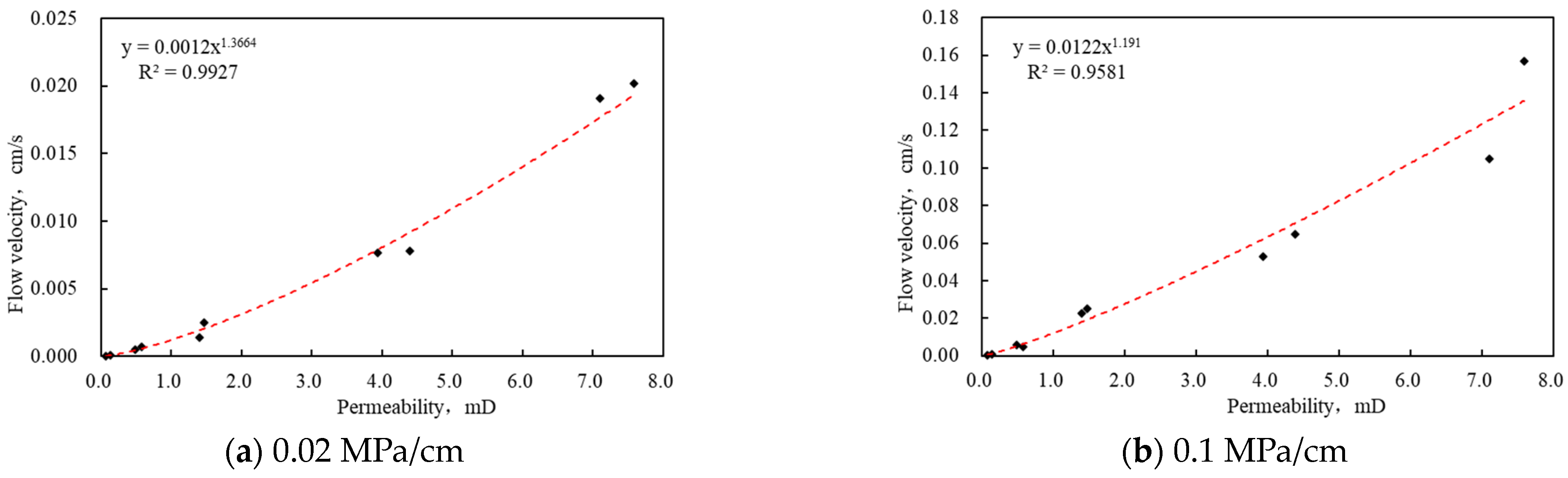
3.2. Experimental Analysis

As shown in Figure 4, based on the seepage characteristics, reservoirs with different physical properties are divided into three regions. When the permeability is less than 1 mD, as the permeability decreases, the coefficient m sharply increases, and the nonlinear seepage characteristics of the core are enhanced. When the permeability is between 1~5 mD, as the permeability increases, the coefficient m gradually decreases and the nonlinear seepage characteristics weaken. When the permeability is greater than 5 mD, the coefficient m remains almost unchanged as the permeability increases, and the nonlinear seepage characteristics are not obvious.

To further investigate the influence of displacement pressure gradient on the seepage flow in tight reservoirs, the fluid flow velocity in different permeability units under different pressure gradient conditions was analyzed, as shown in Figure 5. Based on the experiment data, under the same pressure gradient, the permeability and fluid flow velocity are fitted as follows:

$$v=c_3\cdot K^{c_4}$$

(19)

As shown in Figure 6, the relationship between reservoir permeability and flow velocity under different pressure gradient conditions is shown. The fitting parameters are listed in

Table 4. Fitting parameters between permeability and flow velocity.

Displacement Pressure Gradient (MPa/cm)	Coefficient c3	Coefficient c4	Fitting Degree R
0.02	0.0012	1.3664	0.9927
0.1	0.0122	1.1910	0.9581
0.5	0.0836	1.0358	0.9931
1.0	0.1821	1.0334	0.9997

, the fitting degree is greater than 0.95, indicating a high accuracy of the fitting results. The coefficient c4 reflects the linear relationship between permeability and flow velocity. The larger the coefficient c4 value, the faster the fluid flow velocity increases with the increase in permeability, indicating a more significant nonlinear relationship between permeability and flow velocity. The influence of pressure gradient on nonlinear seepage can also be divided into three parts: when the pressure gradient is less than 0.1 MPa/cm and the coefficient c4 is greater than 1.2, the permeability in tight reservoirs has a significant impact on fluid nonlinear seepage. When the pressure gradient is between 0.1~0.5 MPa/cm, the influence of permeability on nonlinear fluid flow decreases with the increase in pressure gradient. When the pressure gradient is greater than 0.5 MPa/cm and the coefficient c₄ is approximately 1.03, the permeability in a tight reservoir has little effect on the nonlinear flow of fluids.

Therefore, in the process of oilfield development, advanced water injection and energy replenishment can be used to increase reservoir pressure, reduce the impact of low-velocity nonlinear seepage characteristics of underground fluids on reservoir production, and ensure stable production of the reservoir.

4. Nonlinear Seepage Numerical Simulation

As shown in Figure 7, a nonlinear seepage model is established through model derivation and core displacement experiment results, and numerical simulation results are used to guide the water injection development of beach-bar sandstone reservoirs. In different permeability reservoirs, considering the influence of natural fractures, numerical simulation of water injection development in beach-bar sandstone reservoirs is conducted to clarify the impact of nonlinear seepage on water injection pressure conduction and oil well production in the injection production well group, providing guidance for later fracturing–flooding development. As shown in Figure 8, in the model, one water injection well (W1) is injected at a constant flow rate, while four production wells (W2, W3, W4, W5) are produced at a constant bottom hole pressure. The main parameters of the reservoir are shown in

Table 5. Main parameters of oil reservoirs.

Reservoir Parameters	Parameter Value	Reservoir Parameters	Parameter Value
Reservoir depth (m)	3000	Initial oil saturation (%)	60
Reservoir pressure (MPa)	35	Young’s modulus (MPa)	3 × 104
Matrix permeability (mD)	0.5~5	Poisson’s ratio	0.3
matrix porosity (%)	15	Oil compressibility (MPa−1)	6 × 10−4
Natural fracture permeability (mD)	10,000	Water compressibility (MPa−1)	4 × 10−4
Natural fracture porosity (%)	60	Rock compression coefficient (MPa−1)	1 × 10−4
Crude oil viscosity (mPa·s)	10	Crude oil density (kg/m3)	980
Water viscosity (mPa·s)	1	Water density (kg/m3)	1000
Production pressure difference (MPa)	10	Water injection rate (m3/d)	20

. The grid accuracy of this model in the x, y, and z directions is 1, 1, and 0.5 m, respectively. The internal boundary adopts the Dirichlet boundary, and is produced or injected at a constant flow rate in the wellbore. The entire outer boundary adopts a closed boundary (Neumann boundary), limiting the pressure gradient at the outer boundary to zero. The convergence accuracy is 0.05%, and the calculation stops at the end of the simulation time.

By quantitatively comparing the performance of the traditional nonlinear model (Forchheimer/variable starting pressure gradient) with this model,

Table 6. Comparison between this model and traditional nonlinear models.

Model Type	Recovery Rate Error (%)	Calculation Time (s)
Linear model	15.3	57.8
Forchheimer model	9.8	95.7
Variable starting pressure gradient model	8.5	87.9
This model	6.3	84.1

shows that the recovery error (6.3%) of this model is reduced by 36% compared to the classical nonlinear model, and the calculation time is reduced by 12%.

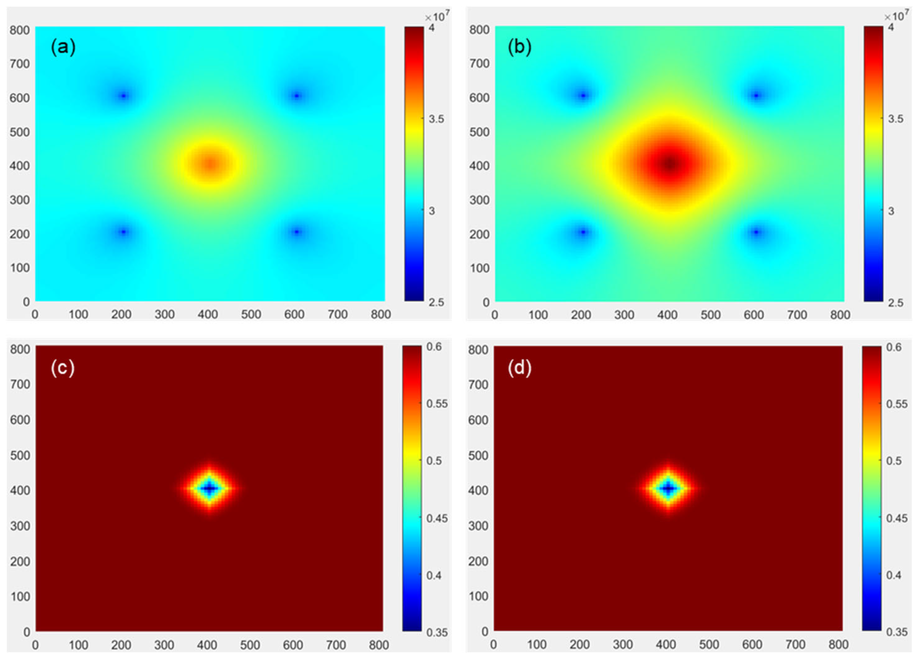
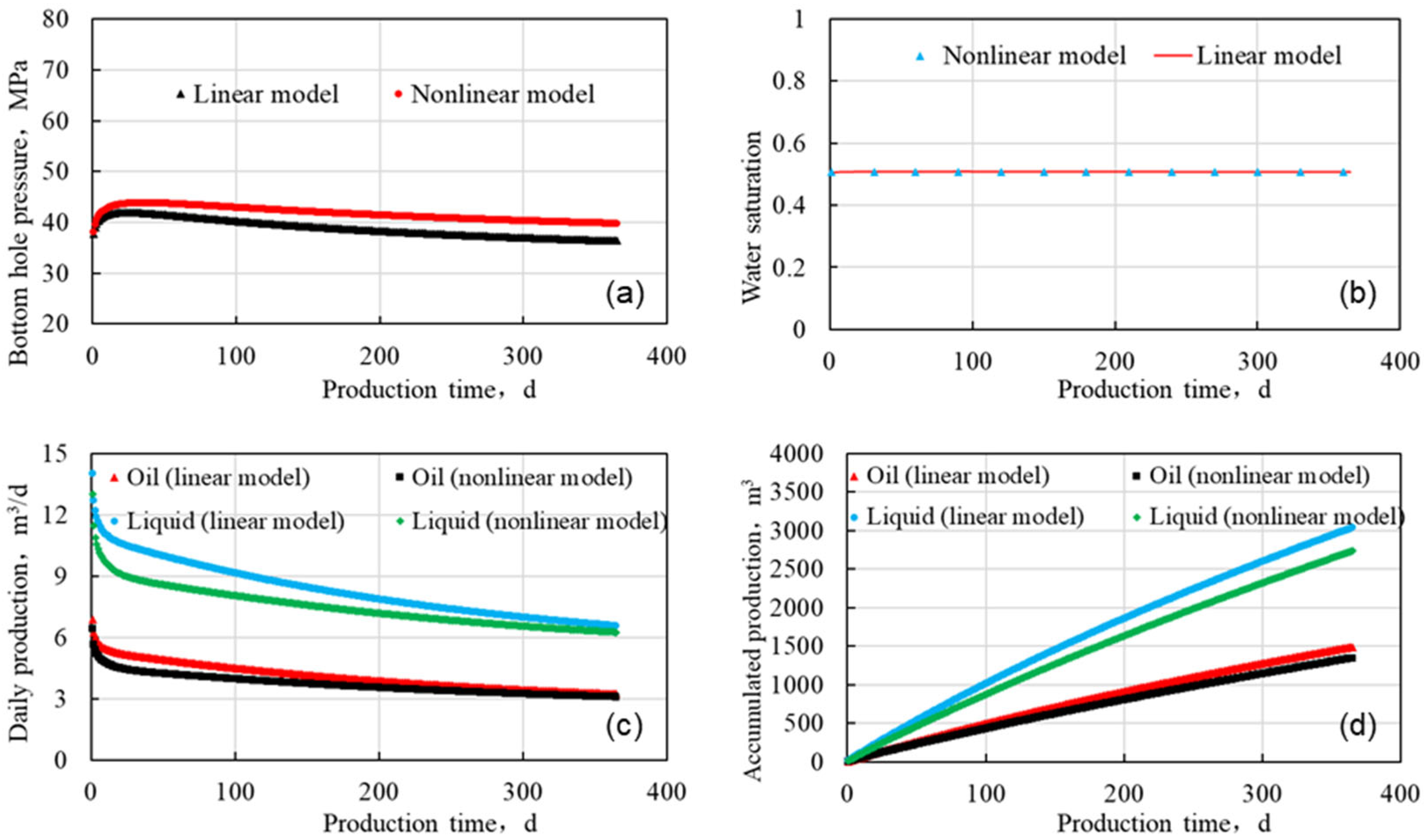
4.1. Beach-Bar Sandstone Reservoir

For the bar sandstone reservoir, the average permeability of the matrix is 5 mD, as shown in Figure 9a,b. During the water injection process, there is a significant difference in the diffusion trend of bottom hole pressure in the injection well between the linear seepage model and the nonlinear seepage model. Under the same injection rate conditions, fluid flow is more difficult in nonlinear seepage models, with injected water gathering around the bottom of the well and resulting in higher bottom hole pressure in the injection well. As shown in Figure 9c,d, under the condition of no fractures, after one year of water injection, the oil and water flow area is small, and the water injection effect range is small. There is no significant difference in the trend of oil saturation changes between linear and nonlinear seepage models. Therefore, during the water injection production process in the bar sandstone reservoir, the fluid nonlinear seepage characteristics are weak, and the fluid nonlinear flow has a slight impact on the water injection pressure conduction process in the bar sandstone reservoir.

As shown in Figure 10a, in the bar sandstone reservoir, due to its good porosity and permeability conditions, when injecting at a water injection rate of 20 m³/d, the filtration rate is greater than the injection rate. Therefore, the bottom hole pressure of the injection well gradually decreases in the later stage of water injection. The nonlinear seepage process affects the pressure transmission between fluids, and the pressure transmission is slower. After one year of water injection, compared to the linear model, the bottom hole pressure of the injection well in the nonlinear seepage model is 3.39 MPa higher (an increase of 9.32%). In this model, the nonlinear seepage characteristics have little effect on the water cut of production wells in the bar sandstone reservoir (Figure 10b).

As shown in Figure 10c, in the bar sandstone reservoir, the transmission of formation pressure is slow, and the bottom pressure of the production well decreases during the production process. Additionally, the daily liquid and oil production of a single well gradually decrease. The daily liquid production of the nonlinear model in the early production stage is 1.82 m³/d lower than that of the linear model. As the production time increases, the daily production of the linear model decreases faster. As shown in Figure 10d, after one year of water injection production, the daily liquid production of the nonlinear model is lower than that of the linear model by 0.3 m³/d (a decrease of 4.58%), the cumulative liquid production decreases by 297.39 m³ (a decrease of 9.8%), the daily oil production decreases by 0.14 m³/d (a decrease of 4.35%), and the cumulative oil production decreases by 145.75 m³ (a decrease of 9.77%).

For beach sandstone reservoirs, the average permeability of the matrix is 0.5 mD. As shown in Figure 11a,b, under the same water injection rate, the nonlinear seepage model has a higher bottom hole pressure in the water injection well and a larger pressure transmission range. There is a significant difference in the pressure diffusion trend between the two models. As shown in Figure 11c,d, under the condition of no fractures, after one year of water injection, there is no significant difference in the trend of oil and water flow between the linear seepage model and the nonlinear seepage model. Due to the poor physical properties of beach sandstone reservoirs, the nonlinear flow characteristics of fluids are strong during the water injection process. The nonlinear flow of fluids has a significant impact on the water injection pressure conduction and oil–water movement patterns in beach sandstone reservoirs, and it is an important influencing factor in the production process of low permeability and tight reservoirs.

As shown in Figure 12a,b, in beach sand reservoirs, due to their poorer porosity and permeability conditions, the water absorption capacity of the reservoir is poor without water injection dynamic fractures. When injecting at a water injection rate of 20 m³/d, the filtration rate of the formation is much lower than the injection rate, so the bottom hole pressure of the injection well continues to rise in the early stage of water injection. After one year of water injection, compared to the linear model, the bottom hole pressure of the injection well in the nonlinear seepage model is 9.13 MPa higher (an increase of 10.56%). Compared to bar sandstone reservoirs, the water injection pressure in beach sandstone ultra-low permeability reservoirs is higher, indicating that water injection is more difficult. Therefore, in the general water injection process of oil fields, the injected water often flows along the high permeability layer of the bar sandstone.

As shown in Figure 12c,d, in the early stage of water injection production in the well group, the water injection pressure has not yet been transmitted to the production well, and the bottom hole pressure of the production well decreases. The daily liquid and oil production of a single well in the production well gradually decrease. In the linear model, when water is injected for 100 days, the injection pressure affects the production well, resulting in an increase in both the daily liquid and oil production of the production well. In the nonlinear model, the transmission of bottom hole pressure in water injection wells is slower. When water injection lasts for 150 days, the injection pressure only extends to the production well, and the daily liquid and oil production of the production well begin to increase. After one year of water injection, the daily liquid production of the nonlinear model was 0.37 m³/d lower than that of the linear model (a decrease of 25.87%), and the cumulative liquid production decreased by 123.17 m³ (a decrease of 27.27%). The daily oil production decreased by 0.18 m³/d (a decrease of 25.71%), and the cumulative oil production decreased by 60.17 m³ (a decrease of 27.13%). Compared to the bar sandstone reservoir, the production of the beach sandstone reservoir is more affected by nonlinear seepage, and the injection production effect is more significantly affected by the nonlinear seepage characteristics of the fluid. Therefore, it is more urgent to reduce the influence of nonlinear seepage characteristics on beach sandstone reservoirs.

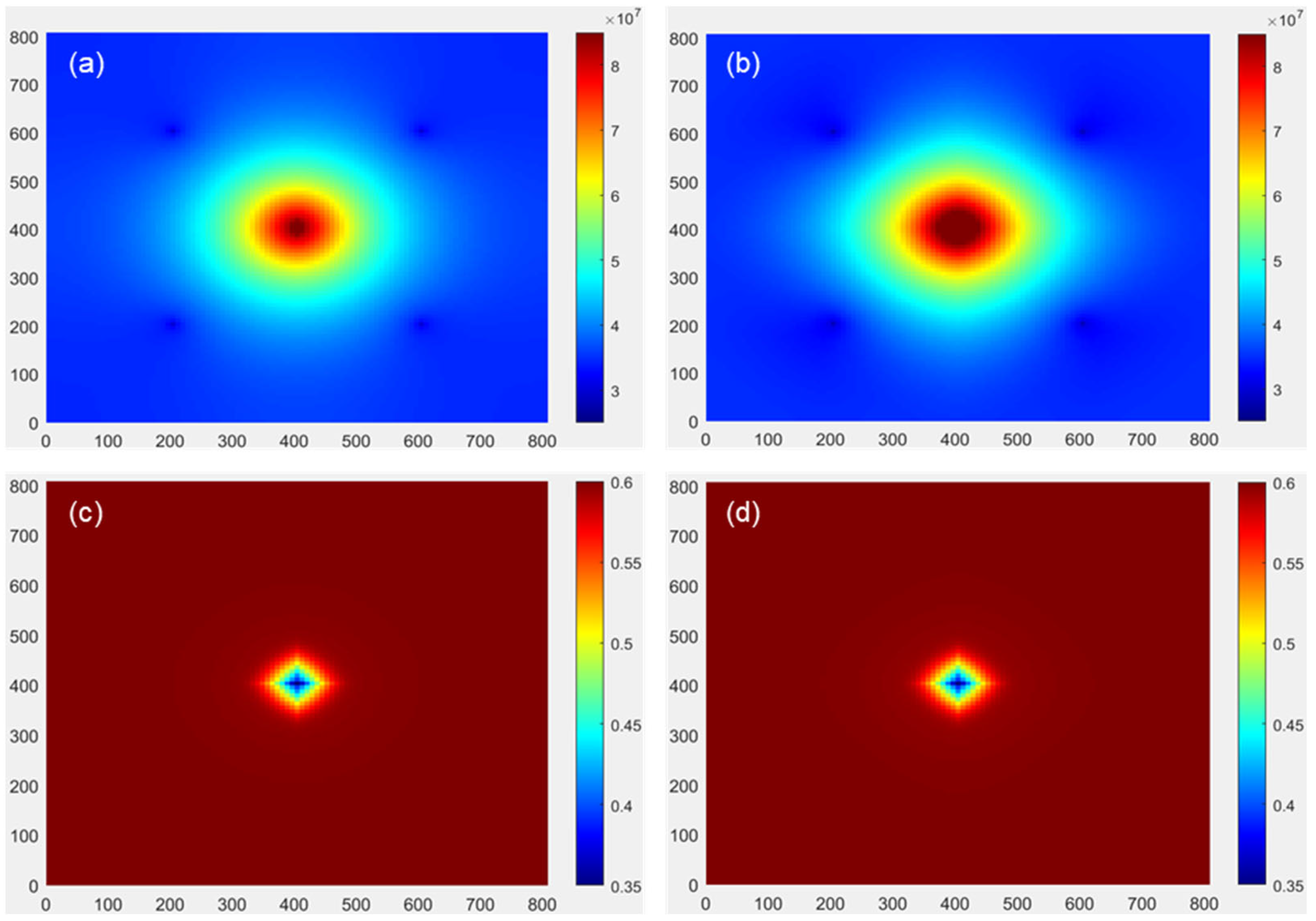
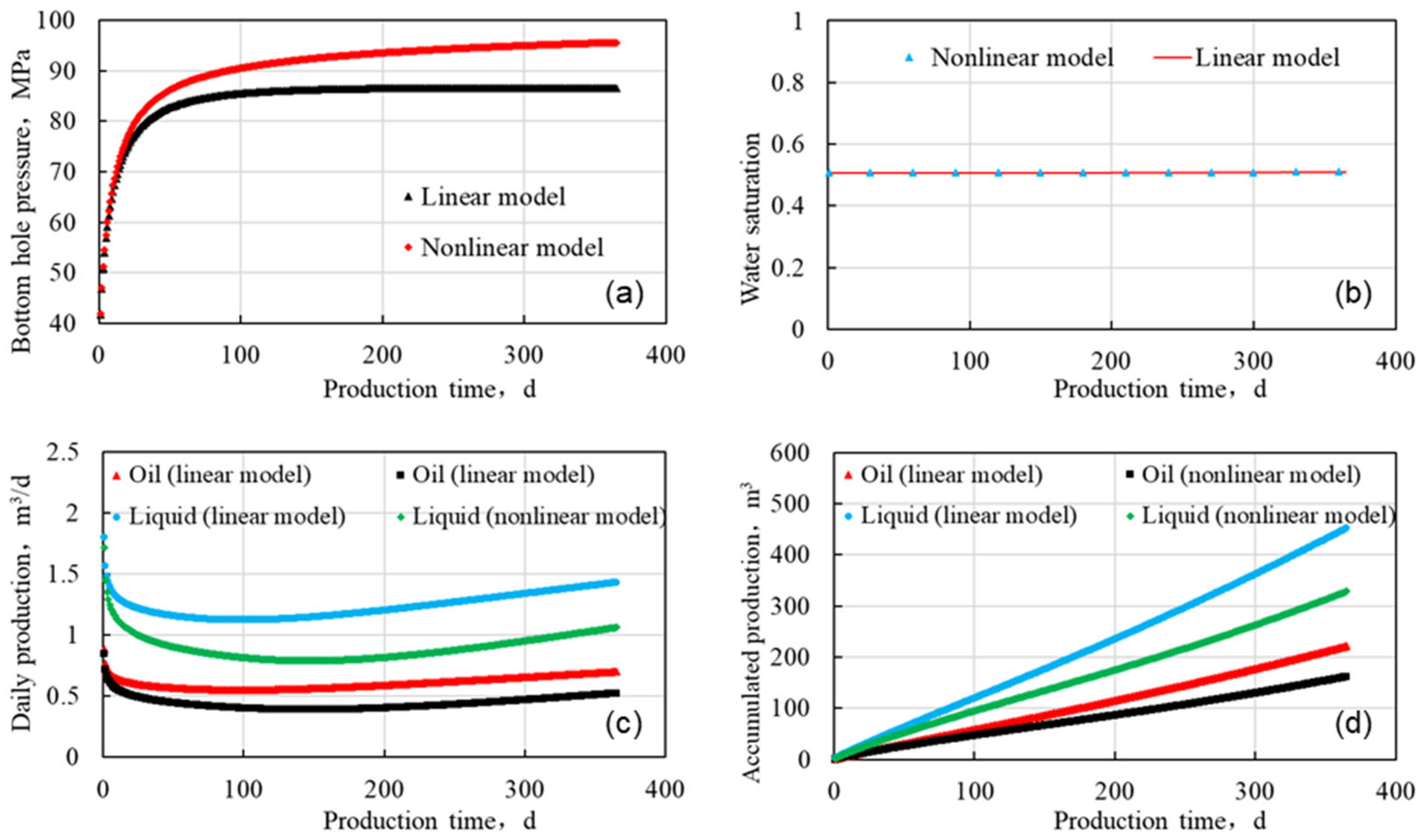
4.2. Natural Fracture Reservoir

Natural fracture reservoir. On the basis of the beach sand reservoir (with a matrix permeability of 0.5 mD as an example), the natural fracture parameters in the beach sand reservoir are set based on the seismic logging data of the reservoir (Figure 13), with a density of 5/100 m, a length of 25 m, and a natural fracture angle of the maximum horizontal principal stress direction (NE30°). Other reservoir parameters are shown in Table 5.

For beach sandstone reservoirs with natural fractures, as shown in Figure 14a,b, the pressure transmission at the bottom of the injection well in the nonlinear seepage model is slower. Under the same water injection rate, the nonlinear seepage model has a higher bottom hole pressure and a wider range of pressure propagation in water injection wells. Affected by natural fractures, the pressure transmission in the reservoir exhibits anisotropic characteristics, indicating faster water injection pressure transmission along the natural fracture direction of the reservoir. The perforation position of production well W3 is located in the natural fracture, and its bottom hole pressure decreases significantly after one year of production. As shown in Figure 14c,d, after one year of water injection, the injected water flows along the natural fracture, and the front edge of the water injection advances rapidly towards the W3 well direction along the natural fracture. Therefore, in the later stage of injection and production, it is necessary to consider blocking the injection direction and adjusting the injection profile of the well group.

As shown in Figure 15a,b, compared to the matrix beach sandstone, the water absorption capacity of the fractured beach sandstone reservoir has been significantly improved, and the initial water injection pressure has decreased by 10 MPa. During the one-year process of water injection, the bottom pressure of the injection well in the linear seepage model decreased from 70.06 MPa to 67.82 MPa, while the bottom pressure of the injection well in the nonlinear model gradually increased and stabilized at around 76 MPa. Compared with the linear model, the bottom pressure of the injection well in the nonlinear seepage model was 8.18 MPa higher (an increase of 12.06%).

As shown in Figure 15c,d, in fractured beach sandstone reservoirs, during the initial stage of well group water injection, the water injection pressure has not yet been transmitted to the production well, and the bottom hole pressure of the production well decreases. The daily liquid and oil production of a single well gradually decrease. After about 50 days of water injection, the injection pressure affects the production well, and the daily liquid and oil production of the production well begin to gradually increase. Compared to matrix type beach sandstone reservoirs, fractured beach sandstone reservoirs have faster pressure transmission and faster production improvement of well groups. After one year of water injection, the average daily liquid production of a single well in the nonlinear model was 0.44 m³/d lower than that in the linear model (a decrease of 12.29%), and the average cumulative liquid production of a single well decreased by 222.16 m³ (a decrease of 18.13%). The average daily oil production of a single well decreased by 0.22 m³/d (a decrease of 12.50%), and the average cumulative oil production of a single well decreased by 109.25 m³ (a decrease of 18.08%). Compared to matrix type beach sandstone reservoirs, natural fractures can effectively weaken the impact of fluid nonlinear seepage characteristics on the injection and production efficiency of beach sandstone reservoirs. Therefore, volume fracturing can be used to break down the reservoir, forming a large-scale fracture network, reducing the impact of nonlinear seepage characteristics in tight reservoirs, and effectively improving the recovery efficiency of beach sand reservoirs.

4.3. Nonlinear Flow Analysis

Based on the fluid flow velocity, injection pressure transfer, and fluid flow mode in the nonlinear seepage model, the beach-bar sandstone reservoir is divided into four flow zones as a whole, as shown in Figure 16a, providing guidance for later reservoir stimulation.

As shown in Figure 16b, the oilfield block is divided into flowing zones and non-flowing zones based on flow velocity. The non-flowing zones in the nonlinear seepage model decreases with pressure diffusion in the early stages of production. After injecting water into the well group for a period of time, the non-flowing area reaches stability. The purpose of fracturing–flooding is to reduce the non-flow zone controlled by the injection production well group and increase the area of the flow zone affected by water injection.

As shown in Figure 16c, according to the seepage mode, the flow area can be divided into Zone I (linear seepage zone) and Zone II (nonlinear seepage zone). The linear seepage zone has a small area and is mainly concentrated around the injection well. The fluid flow velocity is positively correlated with the displacement pressure and flows in a linear manner. The nonlinear seepage zone occupies the vast majority of the well group flow area, and nonlinear seepage is the main form of matrix flow in low permeability beach-bar sandstone reservoirs. For the low-permeability reservoirs stimulation, we can appropriately increase the water injection displacement to generate a dynamic fracture network of water injection, improve the basic physical properties of the reservoir through the fracture network, increase the linear seepage area, and thus reduce the impact of nonlinear seepage characteristics on water injection and oil production effects during injection and production.

As shown in Figure 16d, based on the pressure conduction model, the non-flowing area of oil and water can be divided into Zone III (non-flow zone affected by pressure) and Zone IV (non-flow zone not affected by pressure). The pressure did not reach the area, and due to the low efficiency of pressure transmission in low permeability reservoirs, the pressure could not be transmitted. In the later stage, the pressure coverage range can be expanded by increasing the control range of water injection dynamic fractures. For Zone III, due to the low efficiency of pressure transmission in low-permeability reservoirs, the pressure cannot be transmitted. Therefore, the pressure range can be expanded by increasing the control range of water injection dynamic fractures. For Zone IV, although it is within the influence range of water injection pressure, due to factors such as poor reservoir properties, there is still a phenomenon of oil–water not flowing or a very weak flow trend. For such areas, oil and water displacement can be promoted through measures such as shut in in the later stage, so as to improve the recovery factor of tight reservoirs.

5. Conclusions

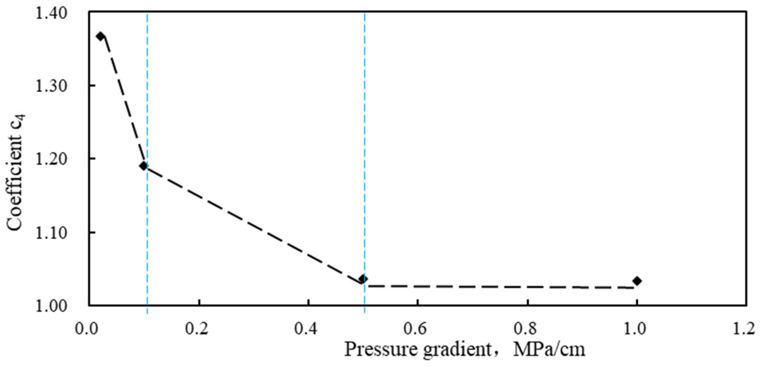
• The displacement pressure and flow rate of beach-bar sandstone reservoirs exhibit a significant nonlinear relationship. The lower the permeability and the smaller the displacement pressure, the more significant the nonlinear seepage characteristics. Based on experimental results, fitting the low-velocity nonlinear seepage coefficient and establishing a low-velocity nonlinear seepage model based on time-varying physical properties can more accurately reflect the underground seepage situation of beach-bar sandstone reservoirs.
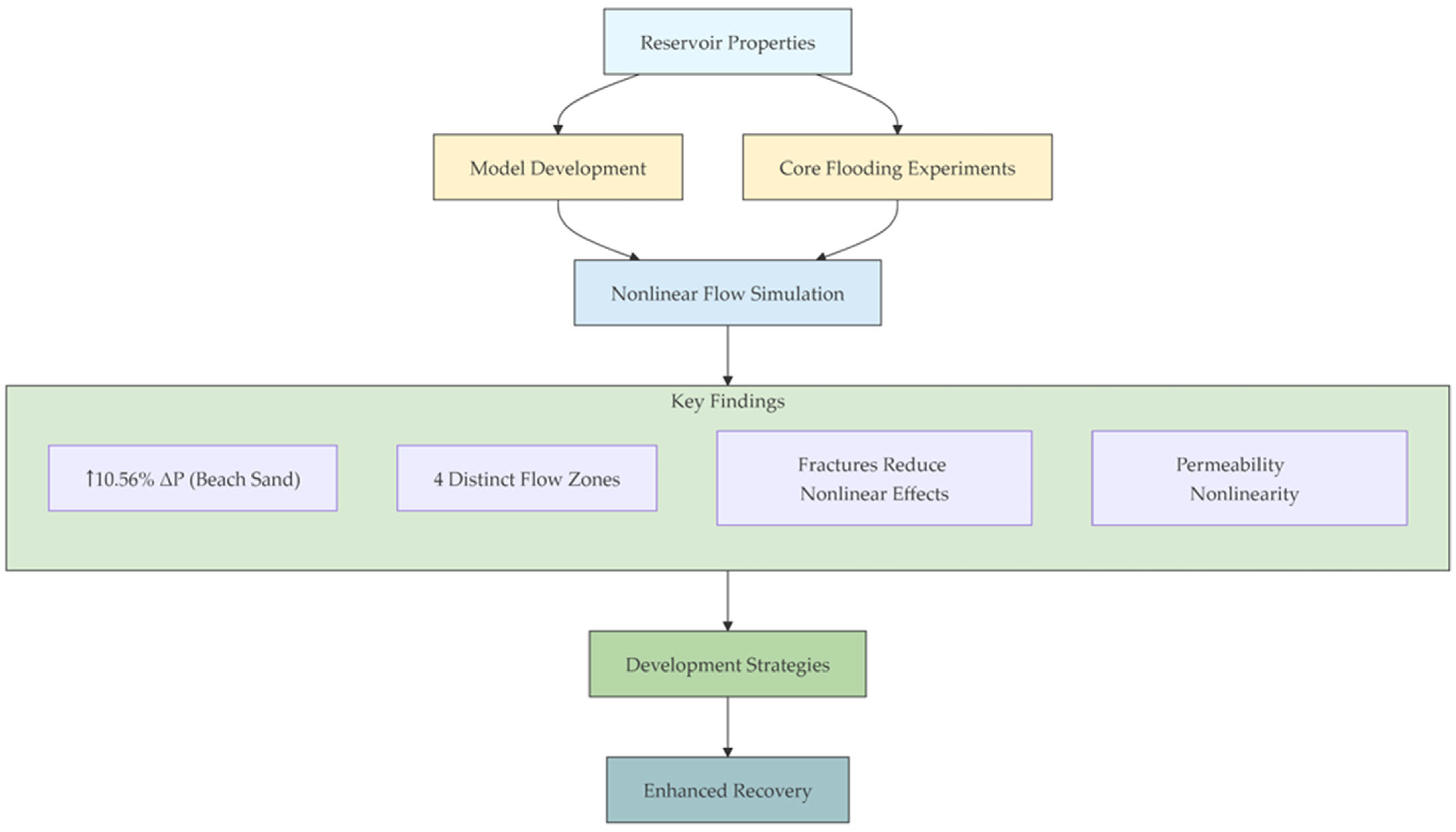
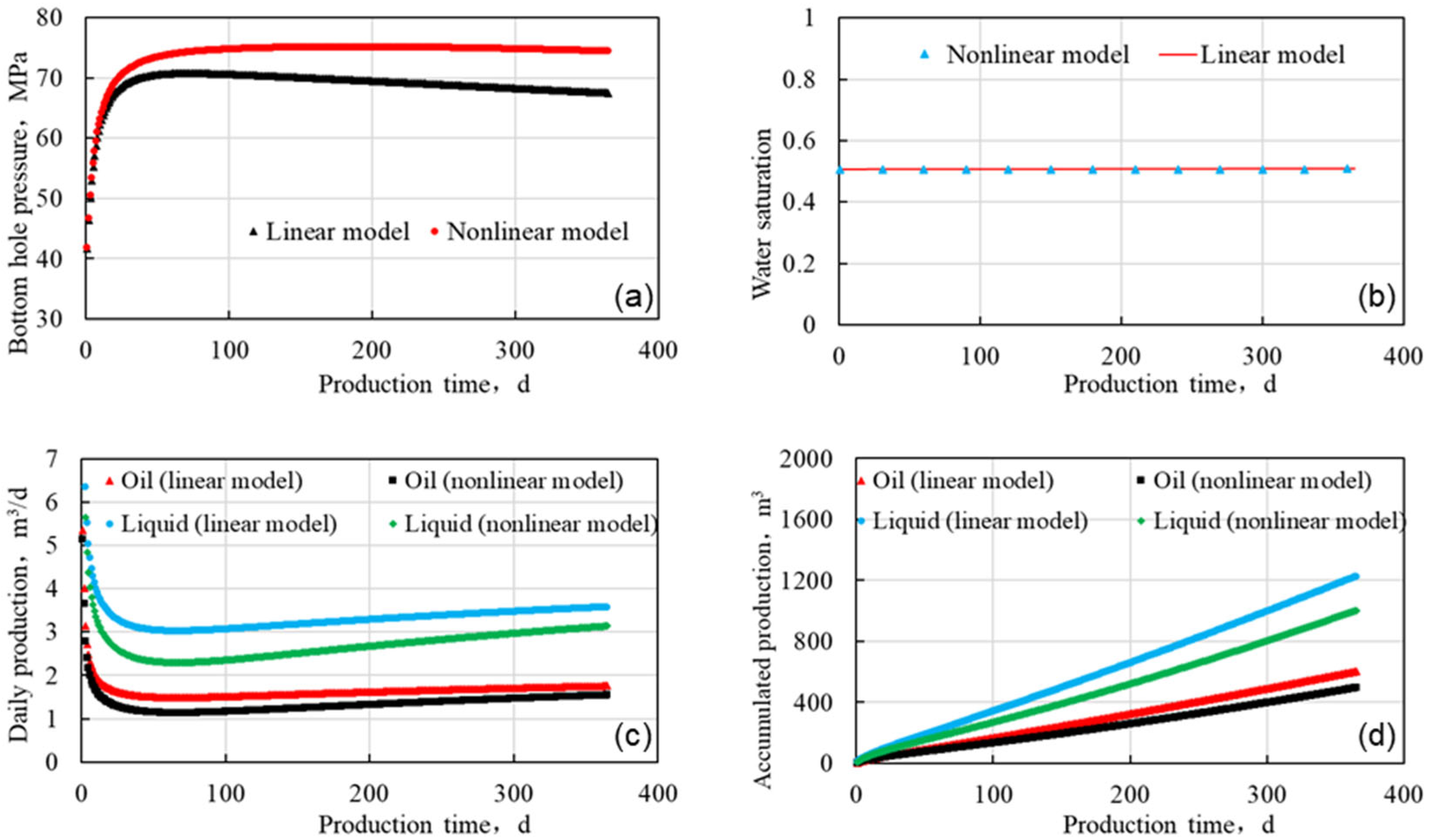
• Compared to the bar sandstone reservoir, the water injection pressure in the beach sandstone reservoir is higher. In the nonlinear seepage model, the bottom hole pressure of the water injection well increases by 9.13 MPa (an increase of 10.56%), indicating that water injection is more difficult. After one year of water injection, the cumulative oil production of the nonlinear model decreased by 60.17 m³, a decrease of 27.13%.
• In fractured sandstone reservoirs, after one year of water injection, the average daily oil production of a single well in the nonlinear model decreased by 0.22 m³/d, a decrease of 12.50%, and the average cumulative oil production of a single well decreased by 109.25 m³, a decrease of 18.08%. Compared to matrix type beach sand reservoirs, natural fractures can effectively reduce the impact of fluid nonlinear seepage characteristics on the injection and production efficiency of beach sandstone reservoirs.
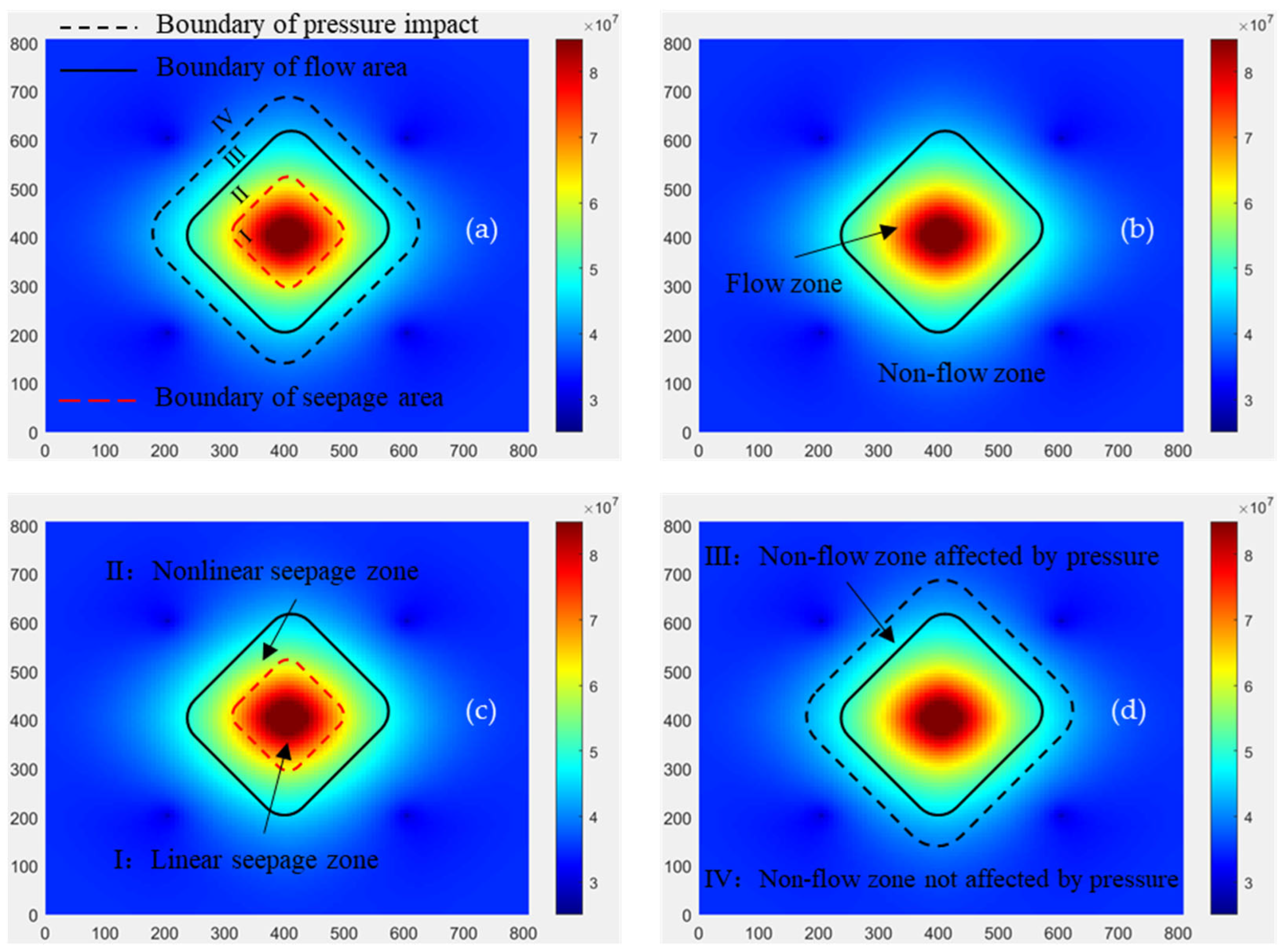
• Based on the fluid flow velocity, injection pressure, and fluid flow mode in the nonlinear seepage model, the beach-bar sandstone reservoir can be divided into four flow zones during the injection–production process, including Zone I (linear seepage zone), Zone II (nonlinear seepage zone), Zone III (non-flow zone affected by pressure), and Zone IV (non-flow zone not affected by pressure).

References

1. Zhang, K.; Zhang, L.Q.; Liu, D.M. Situation of China’s oil and gas exploration and development in recent years and relevant suggestions. Acta Pet. Sin. 2022, 43, 15–28. [Google Scholar]
2. Guo, J.C.; Ma, L.; Lu, C. Progress and development directions of fracturing flooding technology for tight reservoirs in China. Acta Pet. Sin. 2022, 43, 1788–1797. [Google Scholar]
3. Dykstra, H.; Parsons, R.L. The Prediction of Oil Recovery by Water Flood. Secondary Recovery of Oil in the United States, 2nd ed.; API: New York, NY, USA, 1950. [Google Scholar]
4. Li, Q.C.; Li, Y.D.; Cheng, Y.F.; Li, Q.; Wang, F.L.; Wei, J.; Liu, Y.W.; Zhang, C.; Song, B.J.; Yan, C.L.; et al. Numerical simulation of fracture reorientation during hydraulic fracturing in perforated horizontal well in shale reservoirs. Energy Sources Part A Recovery Util. Environ. Eff. 2018, 40, 1486920. [Google Scholar] [CrossRef]
5. Li, Q.; Li, Q.C.; Wang, F.L.; Xu, N.; Wang, Y.L.; Bai, B.J. Settling behavior and mechanism analysis of kaolinite as a fracture proppant of hydrocarbon reservoirs in CO2 fracturing fluid. Colloids Surf. A Physicochem. Eng. Asp. 2025, 724, 137563. [Google Scholar] [CrossRef]
6. Han, Z.; Pidho, J.J.; Yan, C.; Liang, Y.; Cheng, Y. Study on Multiscale Fluid–Solid Coupling Theoretical Model and Productivity Analysis of Horizontal Well in Shale Gas Reservoirs. Energy Fuels 2023, 37, 5059–5077. [Google Scholar] [CrossRef]
7. Fu, Y.; Zhai, Q.; Yuan, G.; Wang, Z.; Cheng, Y.; Wang, M.; Wu, W.; Ni, G. Multi-scale nonlinear reservoir flow simulation based on digital core reconstruction. Geoenergy Sci. Eng. 2024, 242, 213218. [Google Scholar] [CrossRef]
8. Liu, Y.; Zhao, H.; Deng, X.; Guan, B.; Li, J.; Yang, C.; Huang, G. Study on the Seepage Characteristics of Deep Tight Reservoirs Considering the Effects of Creep. Energy Eng. 2025, 122, 063706. [Google Scholar] [CrossRef]
9. Alvaro, P.; Faruk, C. Modification of Darcy’s law for the threshold pressure gradient. J. Pet. Sci. Eng. 1999, 22, 237–240. [Google Scholar]
10. Xu, J.H.; Cheng, L.S.; Zhou, Y.; Ma, L.L. A new method for calculating kickoff pressure gradient in low permeability reservoirs. Pet. Explor. Dev. 2007, 34, 594–602. [Google Scholar]
11. Jiang, R.Z.; Yang, R.F.; Ma, Y.X.; Zhuang, Y.; Li, L.K. Nonlinear percolation theory and numerical simulation in low permeability reservoirs. Chin. J. Hydrodyn. 2011, 26, 444–452. [Google Scholar]
12. Li, L.; Xu, P.; Li, Q.; Zheng, R.Y.; Xu, X.M.; Wu, J.F.; He, B.Y.; Bao, J.J.; Tan, D.P. A coupled LBM-LES-DEM particle flow modeling for microfluidic chip and ultrasonic-based particle aggregation control method. Appl. Math. Model. 2025, 143, 116025. [Google Scholar] [CrossRef]
13. Li, Y.Z.; Duan, B.; Shang, L.; Sun, Y.C.; Gong, L.R.; Xin, C.Y.; Xing, J.P. Numerical simulation method and its application for nonlinear flow in ultra-low permeability and tight oil reservoir in Jidong Oilfield. Pet. Geol. Oilfield Dev. Daqing 2022, 41, 153–158. [Google Scholar]
14. Xu, P.; Li, Q.H.; Wang, C.Y.; Li, L.; Tan, D.P.; Wu, H.P. Interlayer healing mechanism of multipath deposition 3D printing models and interlayer strength regulation method. J. Manuf. Process. 2025, 141, 1031–1047. [Google Scholar] [CrossRef]
15. Cheng, S.Q.; Xu, L.X.; Zhang, D.C. Type curve matching of well test data for non-Darcy flow at low velocity. Pet. Explor. Dev. 1996, 23, 50–53. [Google Scholar]
16. Song, F.Q.; Liu, C.Q.; Hu, J.G. The use of pressure build up data to calculate reservoir starting pressure gradient. Well Test. 1999, 8, 5–7. [Google Scholar]
17. Deng, Y.E.; Liu, C.Q. Mathematical model of nonlinear flow law in low permeability porous media and its application. Acta Pet. Sin. 2001, 22, 72–77. [Google Scholar]
18. Yang, Q.L. The Theory and Application of Nonlinear Seepage Flow in Ultra-Low Permeability Reservoirs; Institute of Percolation and Fluid Mechanics, Chinese Academy of Sciences: Beijing, China, 2007. [Google Scholar]
19. Yuan, Y.R.; Han, Y.Y. Numerical simulation and application of three-dimensional oil resources migration-accumulation of fluid dynamics in porous media. Sci. China Ser. G Phys. Mech. Astron. 2008, 51, 1144–1163. [Google Scholar] [CrossRef]
20. Long, T. Development of a Numerical Simulation System for Non-Darcy Flow in Low Permeability Reservoirs; Tsinghua University: Beijing, China, 2005. [Google Scholar]
21. Huang, Y.Z. Research on the Nonlinear Seepage Mechanism and Variable Permeability Numerical Method of Low Permeability Rock; Tsinghua University: Beijing, China, 2006. [Google Scholar]
22. Jiang, R.Z.; Li, L.K.; Xu, J.C.; Yang, R.F.; Zhuang, Y. A nonlinear mathematical model for low-permeability reservoirs and well-testing analysis. Acta Pet. Sin. 2012, 33, 264–268. [Google Scholar]
23. Deng, Y.E.; Liu, C.Q. Analysis of pressure of nonlinear flow through low-permeability reservoir with vertically fractured well producing. Pet. Explor. Dev. 2003, 30, 81–83. [Google Scholar]
24. Shi, Y.; Yang, Z.M.; Huang, Y.Z. The study of two phase non-linear flow in low permeability reservoir. Mech. Eng. 2008, 30, 16–17. [Google Scholar]
25. Zhu, W.Y.; Li, H.; Deng, Q.J.; Ma, Q.P.; Liu, Y.J. Review on mesoscopic flow theory in porous media. Chin. J. Eng. 2022, 44, 951–962. [Google Scholar]
26. Cao, R.Y.; Cheng, L.S.; Du, X.L.; Shi, J.J.; Yang, C.X. Research progress on fluids flow mechanism and mathematical model in tight oil reservoirs. J. Southwest Pet. Univ. 2021, 43, 113–136. [Google Scholar]
27. Zeng, B.Q.; Cheng, L.S.; Li, C.L. Low velocity non-linear flow in ultra-low permeability reservoir. J. Pet. Sci. Eng. 2011, 80, 1–6. [Google Scholar] [CrossRef]
28. Song, F.Q.; Bo, L.W.; Zhang, S.M.; Sun, Y.H. Nonlinear flow in low permeability reservoirs: Modelling and experimental verification. Adv. Geo-Energy Res. 2019, 3, 76–81. [Google Scholar] [CrossRef]
29. Huang, S.; Yao, Y.D.; Zhang, S.; Ji, J.H.; Ma, R.Y. A fractal model for oil transport in tight porous media. Transp. Porous Media 2018, 121, 725–739. [Google Scholar] [CrossRef]
Figure 1. Typical nonlinear seepage curve [29]. The red solid line represents the nonlinear flow stage, the black solid line represents the linear flow stage, and the dashed line is the graphical auxiliary line. a, b and c represent the starting pressure difference, quasi linear pressure difference, and linear pressure difference, respectively, while d and e represent the starting and ending points of the linear flow stage.
Energies 18 03789 g001
Figure 2. Schematic diagram of displacement device.
Energies 18 03789 g002
Figure 3. The relationship between core flow rate and pressure gradient.
Energies 18 03789 g003aEnergies 18 03789 g003b
Figure 4. Relationship between coefficient m and permeability. The red dotted line represents the trend line, and the blue dotted line represents the partition line.
Energies 18 03789 g004
Figure 5. Relationship between permeability and flow velocity under different displacement pressure gradient conditions.
Energies 18 03789 g005aEnergies 18 03789 g005b
Figure 6. Relationship between pressure gradient and coefficient c4. The black dotted line represents the trend line, and the blue dotted line represents the partition line.
Energies 18 03789 g006
Figure 7. Research thought process diagram.
Energies 18 03789 g007
Figure 8. Schematic diagram of reservoir injection production well network.
Energies 18 03789 g008
Figure 9. The bar sandstone reservoir. (a) Formation pressure in linear seepage model. (b) Formation pressure in nonlinear seepage model. (c) Oil saturation in linear seepage model. (d) Oil saturation in nonlinear seepage model.
Energies 18 03789 g009
Figure 10. The bar sandstone reservoir. (a) Bottom hole pressure of water injection well. (b) Water content of production wells. (c) Daily production of production wells. (d) Accumulated production of production wells.
Energies 18 03789 g010
Figure 11. The beach sand reservoir. (a) Formation pressure in linear seepage model. (b) Formation pressure in nonlinear seepage model. (c) Oil saturation in linear seepage model. (d) Oil saturation in nonlinear seepage model.
Energies 18 03789 g011
Figure 12. The beach sand reservoir. (a) Bottom hole pressure of water injection well. (b) Water content of production wells. (c) Daily production of production wells. (d) Accumulated production of production wells.
Energies 18 03789 g012
Figure 13. Schematic diagram of natural fractures.
Energies 18 03789 g013
Figure 14. The natural fracture reservoir. (a) Formation pressure in linear seepage model. (b) Formation pressure in nonlinear seepage model. (c) Oil saturation in linear seepage model. (d) Oil saturation in nonlinear seepage model.
Energies 18 03789 g014
Figure 15. The natural fracture reservoir. (a) Bottom hole pressure of water injection well. (b) Water content of production wells. (c) Daily production of production wells. (d) Accumulated production of production wells.
Energies 18 03789 g015
Figure 16. (a) Nonlinear seepage reservoir pressure. (b) Flow zones division. (c) Classification of seepage modes. (d) Division of pressure affected zones.
Energies 18 03789 g016