Fault Prediction of Hydropower Station Based on CNN-LSTM-GAN with Biased Data

Abstract

Fault prediction of hydropower station is crucial for the stable operation of generator set equipment, but the traditional method struggles to deal with data with an imbalanced distribution and untrustworthiness. This paper proposes a fault detection method based on a convolutional neural network (CNNs) and long short-term memory network (LSTM) with a generative adversarial network (GAN). Firstly, a reliability mechanism based on principal component analysis (PCA) is designed to solve the problem of data bias caused by multiple monitoring devices. Then, the CNN-LSTM network is used to predict time series data, and the GAN is used to expand fault data samples to solve the problem of an unbalanced data distribution. Meanwhile, a multi-scale feature extraction network with time–frequency information is designed to improve the accuracy of fault detection. Finally, a dynamic multi-task training algorithm is proposed to ensure the convergence and training efficiency of the deep models. Experimental results show that compared with RNN, GRU, SVM, and threshold detection algorithms, the proposed fault prediction method improves the accuracy performance by $5.5\%$, $4.8\%$, $7.8\%$, and $9.3\%$, with at least a $160\%$ improvement in the fault recall rate.

1. Introduction

Hydroelectric power is a kind of environmentally friendly renewable energy, so hydropower stations are of great significance for solving the energy shortage problem in economic development, improving the ecological environment and promoting the coordination and sustainable development of regional economies [1]. Globally, hydropower accounts for approximately $14.7\%$ of total electricity generation, and the installed capacity of hydropower accounts for more than $50\%$ of the global installed capacity of renewable energy. As of 2024, the cumulative installed capacity of hydropower worldwide reached 427 million kilowatts, and the annual electricity generation reached $1.5$ trillion kilowatt-hours. The normal operation of hydropower stations’ equipment is of great significance for ensuring power supply and preventing safety accidents [2,3]. Fault detection is an indispensable step in ensuring the safe and reliable operation of industrial systems [4], such as power transmission, manufacturing industry, and transportation and telecommunication systems. Specially, due to the complexity of hydropower station systems, such as in the large number of equipment and variable operating environment, equipment failures are difficult to completely avoid. This not only leads to significant economic losses but may also cause serious production safety accidents, posing adverse effects on society and the environment.

With the development of intelligence and information technologies, the monitoring systems of hydropower stations are now capable of collecting a large amount of real-time operation data from equipment. These data contain rich information [5,6], providing the possibility for fault prediction. By analyzing these data, potential anomalies and fault signs of equipment can be detected in a timely manner [7], so as to take corresponding preventive measures and avoid the occurrence of accidents.

Traditional fault detection technologies mainly rely on signal processing and statistical methods. The former extracts the characteristics of fault data through time–frequency conversion methods such as wavelet transform [8], the empirical mode decomposition method [9], short-time Fourier transform (STFT) [10], and spectral analysis. The latter mainly uses some multivariate statistical analysis methods, such as partial least squares [11], to calculate the fault thresholds for identifying abnormal data. Although these methods can identify, to a certain extent, the potential faults of equipment, their applicability is mainly limited to scenarios with a limited data scale and a relatively simple system structure. Facing the complex data bias problems commonly existing in the operation environment of hydropower stations, such as large data scale and severely imbalanced sample class distribution, traditional methods face significant technical bottlenecks in terms of the robustness of feature extraction, the stability of model training, and the accuracy of fault diagnosis. Firstly, the extracted data features may not fully reflect the real state of the equipment. Secondly, the calculated fault thresholds may no longer be applicable under new operating conditions, and continuous updates are required to maintain the effectiveness of detection. In addition, the above methods only analyze the fault data, and it is impossible to conduct the same analysis and prediction for the huge amount of normal detection data. That is to say, it is difficult to deal with the nonlinear relationships in the data and the dynamic non-stationary changes in time series, and there are also high requirements for the professional knowledge and experience of operators.

At present, some studies have researched intelligent detection technologies for the increasingly complex faults of hydropower stations. This is mainly based on the breakthroughs and developments of artificial intelligence technologies, among which machine learning is the most representative. A fault detection method is proposed based on support vector machine (SVM) in [12], which is optimized based on the particle swarm algorithm [13], thereby improving the judgment accuracy of the model. An improved random forest algorithm [14] is proposed to achieve accurate fault detection and enhance the processing ability of the detection model through optimized parallel processing methods.

The above-mentioned machine learning models usually have a relatively simple structure, and may not fully capture the complex data features. In contrast, deep learning, which uses neural network models for analysis and prediction, can extract more in-depth feature information from the data, and has significant advantages in handling complex data structures and performing accurate modeling and prediction [15]. Through its multi-layer structure, the neural network automatically learns nonlinear relationships. This enables it to more effectively identify potential fault patterns when facing systems with high complexity and dynamic change characteristics such as hydropower stations. In addition, deep learning models can also adapt to changes in the data and enhance the accuracy and robustness of prediction through learning. For example, a fault diagnosis network based on the convolutional neural network (CNN) architecture was designed [16], and its performance has been greatly improved compared with traditional machine learning methods. A residual CNN algorithm based on Bayesian optimization was studied [17]. This algorithm achieved a significant improvement in model performance by embedding residual connections and automatically optimizing hyperparameters. Stacked attention autoencoder fault monitoring methods [18,19] have been put forward to pretrain the model and derive deep fault features for improving the classification accuracy.

Compared with the CNN and SAE models, the recurrent neural network (RNN) model that can acquire the correlation of time series is more applicable to time series prediction tasks. For example, a power grid fault diagnosis scheme based on feature clustering and RNN [20] has significantly improved the utilization rate of unlabeled samples and the diagnostic accuracy. However, RNN often encounters the issues of gradient vanishing or explosion in deep network training, which limits its ability to learn long-distance temporal dependencies. To overcome this obstacle, the long short-term memory (LSTM) network solves the problem of gradient vanishing by introducing a gating mechanism, learning long-distance temporal dependencies. Then, fault detection models for industrial machines and large-scale multi-machine power systems were developed based on the LSTM architectures [21,22,23]. The advantages of LSTM are mainly the following: Firstly, it has excellent memory ability and can store long-term dependency information in the data. Secondly, the gating design of LSTM ensures the training stability and significantly reduces the risk of gradient vanishing and explosion. Finally, LSTM shows good adaptability to processing sequence data of different lengths. In addition, hybrid ensemble learning methods can improve prediction accuracy generally by combining multiple weak learners [24]; however, their structural homogeneity limits comprehensive feature extraction and introduces computational inefficiencies. Meanwhile, due to the high sensitivity of ensemble learning to the selection of base learners and the quality of data, it is difficult to always ensure a robust and reliable performance in the scenario of hydropower stations. The Transformer model, a deep learning framework built on the self-attention mechanism, excels at capturing long-distance relationships within sequences by leveraging global attention [25,26]. This unique capability enables it to deliver outstanding results in natural language processing (NLP) tasks, with sentiment analysis serving as a notable example. However, its direct application to time series forecasting faces limitations, as the strong local correlations inherent in temporal data fundamentally differ from the global semantic requirements of NLP, causing standard attention mechanisms to potentially overlook local temporal patterns.

On the other hand, the equipment of hydropower stations is usually designed with a large safety margin, which leads to a severely imbalanced distribution of actual fault data compared with normal data. In this situation, it is particularly difficult to extract fault features and conduct effective detection. Although meta-learning [27] and contrastive learning [28] are capable of improving the model’s generalization performance for new tasks, their high complexity may lead to overfitting in new tasks, thus affecting the expected performance of the model. In addition, this type of method has limitations in generalization ability. Even after training, the model may demand a large volume of new task data to attain the desired performance. In this situation, the generative adversarial network (GAN) [29], which was originally used for image processing, has gradually been discovered to have the potential to expand samples. It does not have to consider the adaptability of the model to small sample data. Instead, by simulating the data generation process, it directly creates new samples that are extremely similar to the real fault data in statistical features, thus enriching the fault sample library and providing more data support for the training of the fault detection model.

In response to the challenges faced by the fault detection technology of hydropower stations, this paper proposes a fault detection method for data prediction and enhancement based on CNN-LSTM-GAN to enhance the accuracy of fault detection in hydropower stations. In this case, the specific criticalities are dealing with data credibility, imbalance distribution, prediction accuracy and fault missed detection. The main contributions of the paper are as follows.

• We propose a fault prediction framework for the hydropower station with unbalanced and unreliable data. First, we propose a controllable credibility detection mechanism based on principal components analysis (PCA). This mechanism calculates the credibility of the data by analyzing the main change directions of the monitoring data to reduce the impact of the unreliable data. Then, we utilize the GAN to expand the training fault data of the hydropower station, thereby addressing the issue of insufficient fault data volume and imbalanced data distribution. In addition, the CNN-LSTM network is designed to extract detail data features and the long-term dependencies in the time series data for fault prediction.
• We propose a multi-scale feature extraction network architecture based on joint time–frequency information for fault detection. First, the model extracts the local and global time-domain features of the data by distributing the sample to multiple independent network branches with different depths. Then, we analyze the frequency-domain parameters of the sample sequence using discrete STFT, and the frequency-domain information is used to assist in the time-domain feature for improving fault detection accuracy.
• We propose a dynamic multi-task training algorithm for our deep network framework to ensure the convergence and training efficiency. In this paper, both time series prediction tasks and fault detection tasks are considered, but it is difficult to jointly train the entire network model. Therefore, we dynamically adjust the proportion between the prediction sub-network loss and the global detection network loss during each training iteration. This allows the model to focus more on fine-grained subtask errors in the early stages, and gradually shift attention to the global fault detection objective as training progresses.
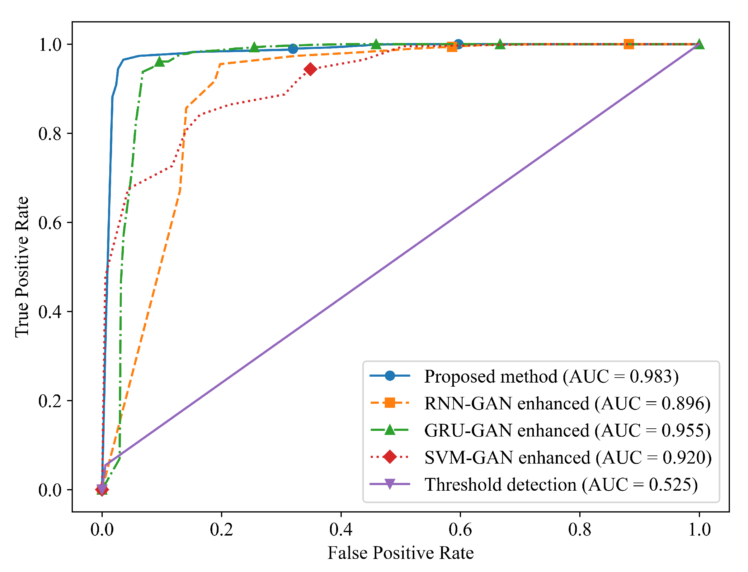
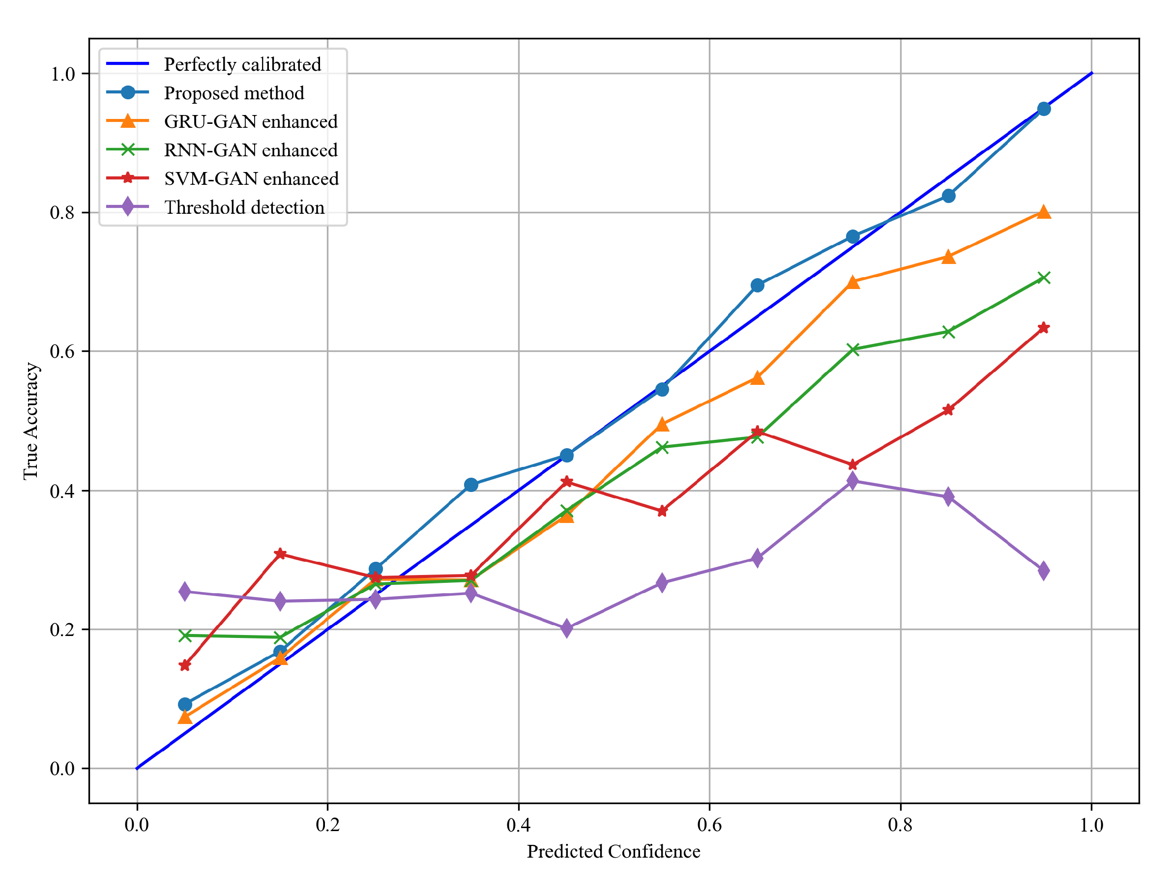
• The proposed method improves the detection accuracy compared to the existing schemes within a manageable time cost. In particular, our method has a significant improvement in recall performance, which is of great significance in scenarios with low fault tolerance and imbalanced data such as hydropower stations.

2. Fault Detection Method Based on CNN-LSTM-GAN

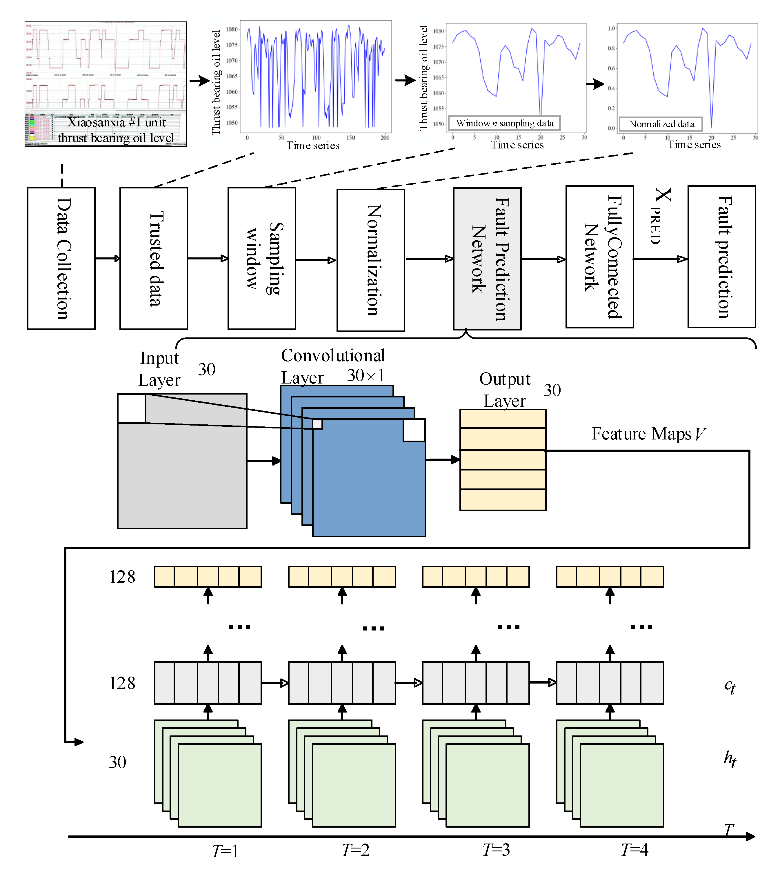
The process of the proposed fault detection method for hydropower stations is illustrated in Figure 1. Firstly, a controllable credibility detection mechanism is designed to analyze the mainstream data trends of the same monitoring data, calculate the credibility of different monitoring data, and screen out the dataset with the highest credibility to ensure the accuracy of the simple data and the efficiency of network training. Then, the dataset is normalized, and the normal monitoring data are sampled according to a time window with a length of n to capture the time series characteristics of the data.

The sampled data is subsequently input into the CNN-LSTM network for accurate prediction, and the GAN is utilized to generate new samples with statistical characteristics similar to real fault data for data augmentation. Finally, in order to grasp the global features of the detection data and make fault evaluation more accurate, a multi-scale deep neural network (DNN) model is designed to extract and classify the features of the data predicted by the CNN-LSTM network, so as to determine whether there is fault data in the predicted data and output the fault identification results accordingly. If there is no fault, the sampling window is returned to continue predicting and inspecting the next batch of data.

2.1. Data Prediction Model Based on PCA and CNN-LSTM

2.1.1. Data Credibility Detection Based on PCA

Before formal data prediction, data screening and preprocessing are required. In this study, a controllable credibility mechanism is adopted for data screening, which mainly includes two key steps: data analysis and feature selection. Firstly, principal component analysis is utilized to identify the main change directions of the monitoring data, due to its key feature extraction capability [30] and the statistical distribution of data samples. By calculating the component matrix P and the proportion of explained variance $\lambda$, the data are projected into a new coordinate system, so as to find the direction with the largest variance, that is, the principal component. These principal components represent the main change patterns of the data and help to identify the structure of the data. Then, we calculate the contribution degree of each group of monitoring data to the PCA results to evaluate the credibility of the data as

$$B_i=\sum _{j=1}^J\left(P_{j,i}^2{\lambda }_j\right),$$

(1)

where $B_i$ is the contribution degree of the i-th group of monitoring data to the PCA result. J is the number of principal components, $P_{j,i}$ is the load of the j-th component for the corresponding variable of the i-th group of data, and ${\lambda }_j$ is the variance of the j-th component. Then, sort each group of monitoring data according to these contribution degrees and assign selection probabilities. The higher the contribution degree of the data, the greater the probability of being selected. In the PCA, normal data, that is, data with the main change pattern, have a greater weight when calculating the contribution degree. By screening out the dataset with the highest contribution degree, those data that best conform to the main change pattern of the data are actually selected, thus ensuring the accuracy and reliability of the subsequent network training.

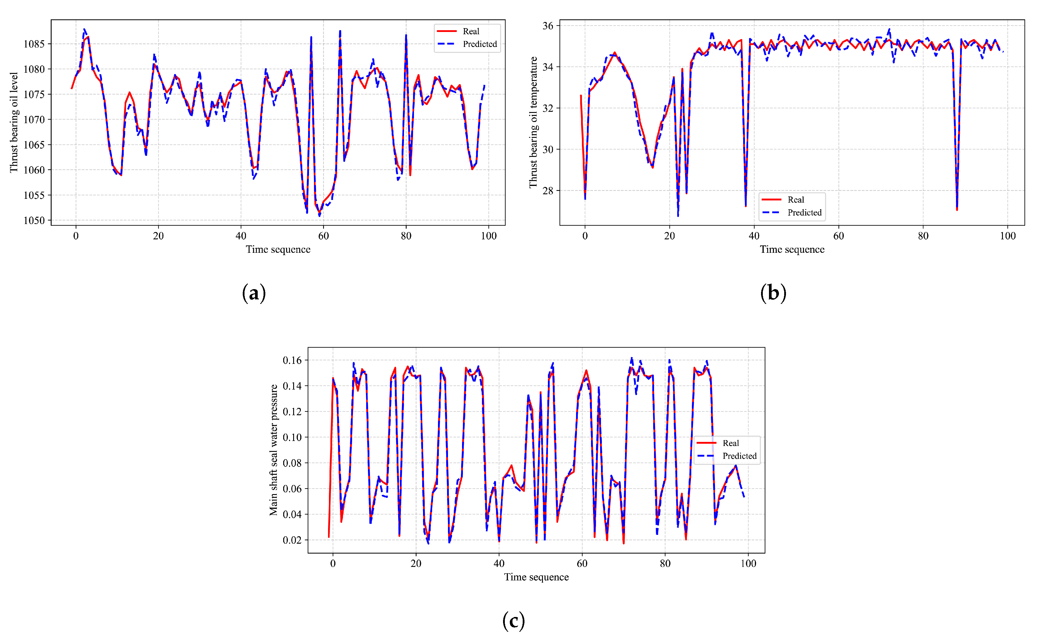
2.1.2. CNN-LSTM Data Prediction

The data are normalized as a preprocessing step. The structure of this prediction model is provided in Figure 2. This model possesses the advantages of both a CNN and LSTM, extracting features from the monitoring data and using a gating mechanism to control the transmission state, thereby maintaining long-term memory of certain features. The network structure mainly consists of CNN layers, LSTM layers, and fully connected layers. The network’s input dimension, represented by the window size n, is configured as 30. This indicates that the model utilizes historical data from the past 30 time steps to predict the value at the subsequent ($31\mathrm{st}$) time step. Given the 2 min sampling interval, this window size corresponds to 1 hour of temporal coverage. This parameter selection achieves an optimal balance between capturing meaningful temporal patterns and maintaining computational efficiency by preventing oversampling-induced redundancy [31].

The input data shape of the network is [BatchSize, Channels, SequenceLength], where BatchSize refers to the batch size, which is 32. Channels refers to the number of input data channels, i.e., the feature dimension. SequenceLength is the sequence length, which is 30. Since the input sequence contains data from 30 time steps, with each time step corresponding to one channel, the total number of input channels is also 30. The kernel size is set to 1, indicating that this CNN layer performs cross-channel weighted fusion of data at each time step (with weights shared across all time steps). This design integrates multi-channel information through linear transformation to provide fused features for the subsequent LSTM layer, rather than extracting local temporal patterns. By performing convolution operations using the predefined kernels over the input sequence, the network generates output features that maintain the same dimensionality as the input data. These feature maps can be represented as

$$V=z\left(\sum _i{w}_i{x}_i+b\right),$$

(2)

where $w_i$ and $x_i$ represent the convolution kernel weights and the input matrix, respectively. z is the activation function, b is the bias parameter, and i is the element index. After several layers of convolution and pooling operations, the resulting feature maps are sequentially flattened into a vector, which is then fed into the fully connected layer as the final output.

Next, the LSTM layer receives the output from the convolutional layer as its input. The hidden state and cell state are then initialized with the shape [NumLayers, BatchSize, HiddenSize]. In this model, there are three hidden layers, each containing 128 neurons. This design ensures the model has sufficient learning capacity while also being able to capture complex patterns within the sequence. Compared to a standard RNN, which only has a single hidden state $h_t$, the LSTM introduces a distinctive cell state $c_t$. This cell state evolves slowly throughout the sequence, allowing important temporal features to be retained over long periods or forgotten when necessary. To manage this cell state effectively, the LSTM includes three key gating units. They work together to determine how the cell state is updated and how the final hidden state is produced. During computation in this prediction network, each gate multiplies the input vector by a weight matrix, and the result is processed by an activation function. The outcome is a value between 0 and 1, which serves as the gate activation controlling the information flow. This architecture allows the LSTM to flexibly and effectively capture key features in time series data, especially when dealing with long sequences.

The forget gate selectively removes information from the prior cell state that is no longer relevant, based on the current input. So, the model can focus on retaining critical information while freeing up memory capacity to incorporate new data. The gating mechanism of the forget gate is expressed as

$$F_t=\sigma \left(W_f[x_t,h_{t-1}]+b_f\right),$$

(3)

where $F_t$ is the current value of the forget gate. $\sigma$ is the activation function, $W_f$ is the weight matrix of the forget gate, and $x_t$ is the input vector at t. $h_{t-1}$ is the hidden state vector from $t-1$, and $b_f$ is the bias vector of the forget gate.

The input gate plays a filtering role. It selects useful information from the current input that is relevant to the prediction and incorporates it into the new candidate cell state. This process ensures that the cell states are continuously updated with the most recent sequence information. The first step involves using the sigmoid function $\sigma$ to determine the weight of information $I_t$ being accepted as

$$I_t=\delta \left(W_i[x_t,h_{t-1}]+b_i\right).$$

(4)

Next, the candidate cell state $C_t^{\prime }$ that contains the new information is

$$C_t^{\prime }=tanh\left(W_c[x_t,h_{t-1}]+b_c\right).$$

(5)

The output gate is responsible for determining which information needs to be transmitted to the hidden state, or to serve as the current model output. These updated pieces of information are passed to the next layer or directly used as the output of the model as

$$Q_t=\delta \left(W_o[x_t,h_{t-1}]+b_o\right).$$

(6)

The updates of the hidden state and the cell state shown above are

$$h_t=O_t\odot tanh\left(C_t\right),$$

(7)

$$C_t=F_t\odot C_{t-1}+I_t\odot C_{t-1}^{\prime },$$

(8)

where ⊙ represents element-wise multiplication, $C_{t-1}$ is the cell state at time $t-1$, and $C_{t-1}^{\prime }$ is the candidate state at the previous moment $t-1$. Through this ingenious gating mechanism, the LSTM can not only effectively capture the long-term dependencies but also avoid gradient vanishing or explosion. Consequently, it can model the long-distance dependencies in the data more accurately.

Finally, the network includes a fully connected layer with a shape of [BatchSize, HiddenSize]. The hidden layer has 128 neurons, and its function is to map the output of the LSTM layer to a single neuron for predicting future data values.

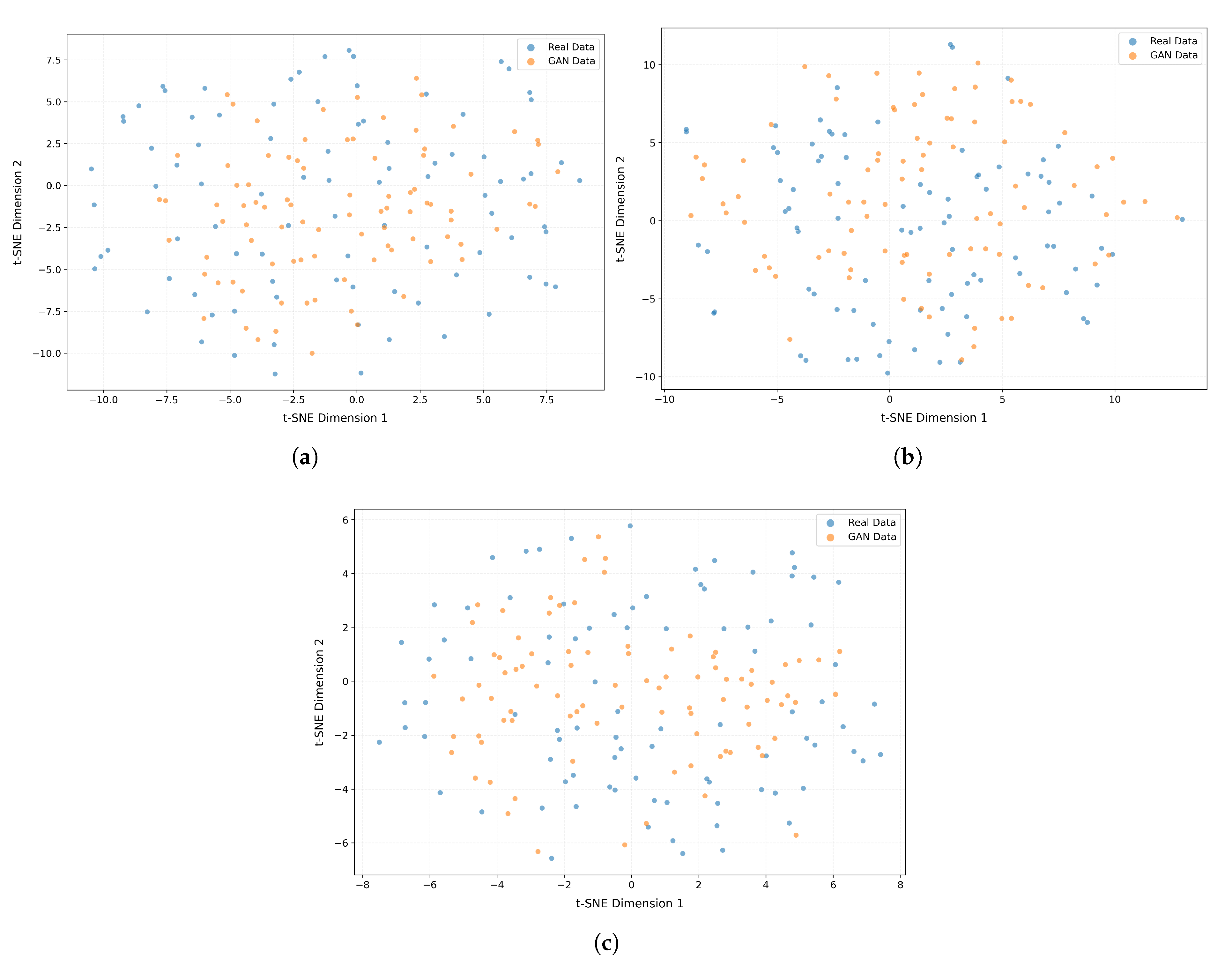
2.2. Fault Data Augmentation Model Based on GAN

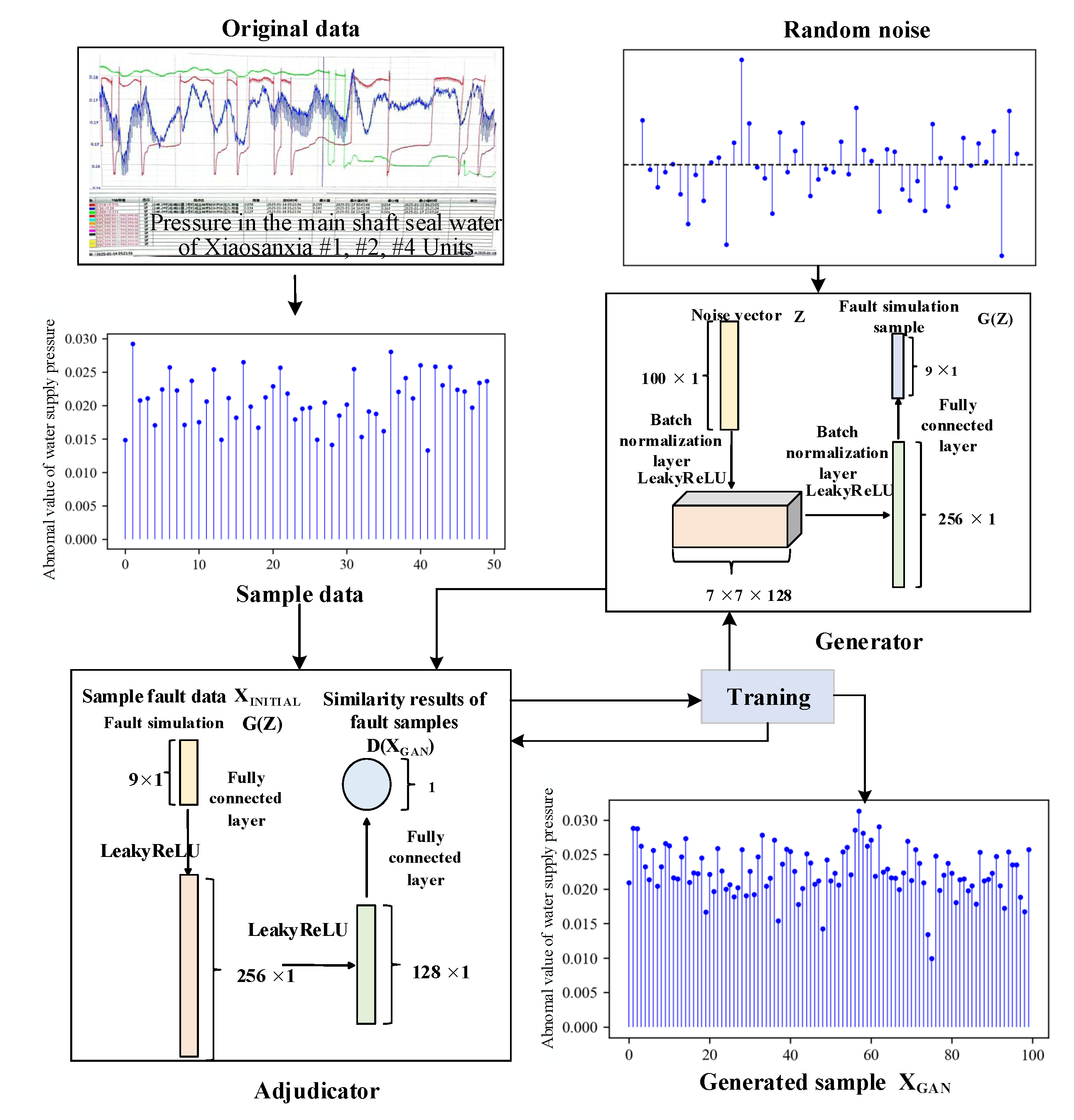
The hydropower fault data enhancement model based on GAN is shown in Figure 3. It mainly consists of two modules: the generator $\mathcal{G}$ and the discriminator $\mathcal{D}$ [32]. During the training process of the model, a unique and dynamic adversarial relationship is formed between $\mathcal{G}$ and $\mathcal{D}$. The responsibility of $\mathcal{G}$ is to create new data through algorithms. Its goal is to mimic the real-world data to deceive the discriminator $\mathcal{D}$. $G\left(z\right)$ represents the data generated by $\mathcal{G}$, where z is a random noise vector. This noise vector is mapped to a vector of shape $(7,7,128)$ through a fully connected layer. Subsequently, the batch normalization (BN) layer normalizes the output of the previous layer.

Immediately afterwards, the leaky rectified linear unit (Leaky-ReLU) activation function provides a non-zero gradient for negative input values. This characteristic helps mitigate the gradient vanishing and maintains the nonlinearity during training. To further improve the performance of the generator, a second fully connected layer with 256 units is incorporated into the model. Finally, the output layer uses the $tanh$ activation function to activate the generated data, restricting the output values to the range of $[-1,1]$. Such a restriction helps match or limit the range of the generated data, making it closer to the distribution of the real fault data. The input layer receives data samples from the generator or the dataset and utilizes a fully connected layer to derive features from the input data. The Leaky-ReLU layer and the Dropout layer are used to introduce nonlinearity and regularization techniques, respectively, reducing the risk of model overfitting. In the output layer generating a scalar value, the $Sigmoid$ function is used to compress the output within the range of $[0,1]$. Among them, a value close to 1 indicates that the model considers the input to be real, while a value close to 0 indicates that the input is generated. The objective function is

$$\underset{G}{min}\underset{D}{max}V(G,D)={\mathbb{E}}_{z\in p_z\left(z\right)}\left[log(1-D(G\left(z\right)\left)\right)\right]+E_{x\in p_{data}\left(x\right)}\left[log\left(D\right(x\left)\right)\right],$$

(9)

where x represents the actual data, $p_{data}\left(x\right)$ describes the distribution of this data, and $\mathbb{E}$ denotes the expectation. Variable z refers to Gaussian random noise, with $p_z$ as its distribution. $\mathcal{D}$ evaluates the generated data, yielding $D\left(G\right(z\left)\right)$, and similarly assesses real data, producing $D\left(x\right)$. The discriminator’s outputs are fed back to the generator, guiding it to create more precise and lifelike data. Through this adversarial training mechanism, the generator and discriminator iteratively improve in a competitive process. Eventually, when the GAN objective function stabilizes, the generator can generate increasingly realistic data that cannot be accurately distinguished, thus achieving the global optimum.

As the training progresses continuously, $G\left(z\right)$ becomes closer and closer to the real data, and the discriminative ability of $\mathcal{D}$ is also constantly improving. In this mutually adversarial process, the capabilities of both $\mathcal{G}$ and $\mathcal{D}$ are enhanced. Under the ideal training state, $\mathcal{G}$ can eventually create fake data that is almost indistinguishable from the real data. For the discriminator $\mathcal{D}$, since the data given by $\mathcal{G}$ are already very realistic, $\mathcal{D}$ will be hesitant when judging these data; that is, $D\left(G\right(z\left)\right)$ is close to $0.5$, indicating that the discriminator cannot determine whether these data are real or fake. Finally, a batch of generated fault values that are close to the real fault values are obtained.

2.3. Fault Detection Model Based on Multi-Scale Feature Network

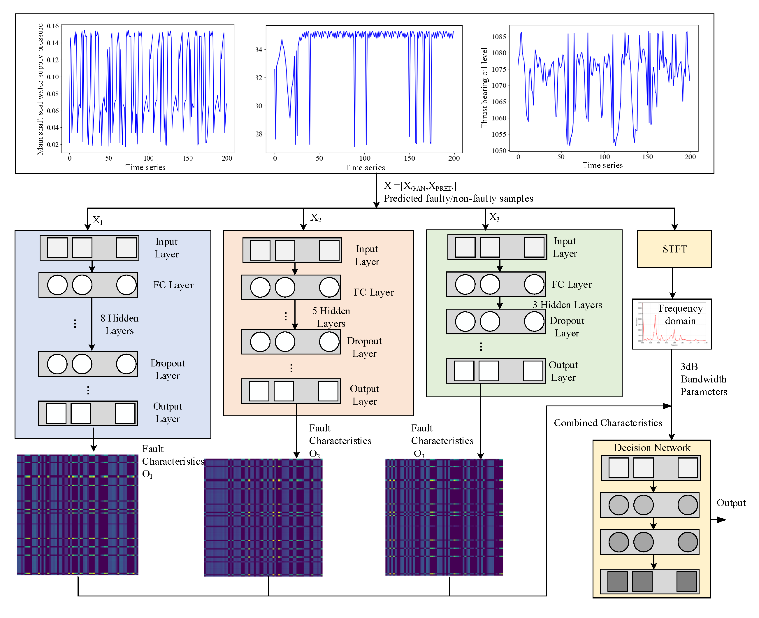
After the above process is completed, the batch of generated fault data is mixed with the predicted data of the CNN-LSTM, and then fed into the multi-scale feature extraction fault detection network for training, so as to enhance the recognition accuracy of the fault detection network. The trained multi-scale feature extraction network is used to conduct fault detection on the predicted values output by the CNN-LSTM network, and the detection results are output. The structure of this network is illustrated in Figure 4. The same input data enters the network through three branches. Each sub-network independently processes the received data and extracts fault features. These features form a collection of all sub-network features through a merging layer. Subsequently, this collection is processed by the hidden layer again, and finally, the fault detection results are output.

The hidden layer of each sub-network is composed of several fully connected layers and Dropout layers. The former are responsible for learning the nonlinear relationships among the input data. As the learning progresses, the output dimensions of these layers will vary. In this network, from left to right, the sub-networks have three, five, and eight hidden layers, respectively, which reflects the extraction of features at different levels and depths, and increases the diversity of the model. When the features of these sub-networks are fused, since each sub-network focuses on different parts of the dataset, the fused features can provide a more comprehensive perspective. This fusion can also enhance the generalization ability, enabling the model to have better detection performance on unseen data, thereby enhancing the robustness.

In addition to the mixed time-domain features, we also use the frequency-domain parameters of the sample data, such as frequency peak position and 3 dB bandwidth, as auxiliary information to assist the model in making its diagnosis. Therefore, incorporating spectrograms as auxiliary inputs into the classification network can improve both the accuracy and robustness of fault detection. We employ the STFT,

$$X(m,\omega )=\sum _{i=-\infty }^{\infty }x\left[i\right]·w[i-m]·e^{-j\omega i},$$

(10)

to extract frequency-domain features from time series signals, where $x\left[i\right]$ denotes the time series signal, $w\left[i\right]$ is the sliding window function, m represents the time shift, and $\omega$ is the frequency variable. In practical applications, the discrete form is typically used as

$$X(m,k)=\sum _{i=0}^{I_f-1}x\left[n\right]·w[i-m]·e^{-j2\pi ki/I_f},$$

(11)

where $I_f$ is the number of samples. By applying the Fourier transform to each time window, a time–frequency representation is obtained, which is then used to enhance the discriminative performance of the multi-scale network.

2.4. Dynamic Multi-Task Training Algorithm

To ensure the convergence and training efficiency, we propose a dynamic multi-task training algorithm, as shown in Algorithm 1. We define the loss functions of the prediction network based on the CNN-LSTM for the regression task and the detection network based on multi-scale DNN for the classification task as ${\mathcal{L}}_s$ in SubNet and ${\mathcal{L}}_g$ in GlobalNet, respectively. We jointly optimize the parameters $\theta$ of the SubNet and GlobalNet. The algorithm initializes the following inputs: training set ${\mathcal{D}}_{\mathrm{train}}=\left\{(X_b,Y_b,L_b)\right\}$, validation set ${\mathcal{D}}_{\mathrm{val}}=\left\{(X_v,Y_v)\right\}$, maximum training steps N, early stopping patience P, and minimum improvement threshold $\delta$. Finally, it outputs the optimal parameters ${\theta }^{*}$. After initializing network parameters, the dynamic weight coefficients are generated at each training iteration step n as

$${\alpha }_s={\displaystyle \frac{1}{\sqrt{n}}},{\alpha }_g=1-{\alpha }_s,$$

(12)

where ${\alpha }_s$ decays with training steps to prioritize the subnet task, while ${\alpha }_g$ increases to amplify the global task influence, enabling a progressive shift in learning focus from local features to global semantics.

Algorithm 1 Dynamic Multi-Task Training Algorithm

1: Input: Training data ${\mathcal{D}}_{\mathrm{train}}$, Validation data ${\mathcal{D}}_{\mathrm{val}}$, Max training steps N, Early stop patience P, Min improvement threshold $\delta$. 2: Output: Optimized parameters ${\theta }^{*}$. 3: Initialize ${\theta }_{\mathrm{global}}$, ${\theta }_{\mathrm{sub}}$, $n\leftarrow 0$, best $\leftarrow \infty$, and ctr $\leftarrow 0$. 4: while $n<N$ and ctr $<P$ do 5:     $n\leftarrow n+1$ 6:     ${\alpha }_s\leftarrow {\displaystyle \frac{1}{\sqrt{n}}}$ 7:     ${\alpha }_g\leftarrow 1-{\alpha }_s$ 8:     for each batch $(X_b,Y_b,L_b)\in {\mathcal{D}}_{\mathrm{train}}$ do 9:         $Y_p\leftarrow \mathrm{SubNet}(X_b;{\theta }_{\mathrm{sub}})$ 10:         $L_p\leftarrow \mathrm{GlobalNet}(X_b;{\theta }_{\mathrm{global}})$ 11:         ${\mathcal{L}}_s\leftarrow {\parallel Y_p-Y_b\parallel }_2^2$ 12:         ${\mathcal{L}}_g\leftarrow -{\displaystyle \sum _i}{L}_b^{\left(i\right)}log{L}_p^{\left(i\right)}$ 13:         $\mathcal{L}\leftarrow {\alpha }_s{\mathcal{L}}_s+{\alpha }_g{\mathcal{L}}_g$ 14:         $\theta \leftarrow \mathrm{Opt}\left(\theta ,{\nabla }_{\theta }\mathcal{L}\right)$ 15:     end for 16:     ${\mathcal{L}}_v\leftarrow 0$ 17:     for each $(X_v,Y_v)\in {\mathcal{D}}_{\mathrm{val}}$ do 18:         ${\mathcal{L}}_v\leftarrow {\mathcal{L}}_v+{\parallel \mathrm{SubNet}\left(X_v\right)-Y_v\parallel }_2^2$ 19:     end for 20:     ${\mathcal{L}}_v\leftarrow {\mathcal{L}}_v/\left|{\mathcal{D}}_{\mathrm{val}}\right|$ 21:     if ${\mathcal{L}}_v<\mathrm{best}-\delta$ then 22:         best $\leftarrow {\mathcal{L}}_v$ 23:         ${\theta }^{*}\leftarrow \theta$ 24:         ctr $\leftarrow 0$ 25:     else 26:         ctr $\leftarrow \mathrm{ctr}+1$ 27:     end if 28: end while 29: return ${\theta }^{*}$.

During training, each batch undergoes forward propagation to obtain the subnet regression predictions $Y_p$ and global network classification predictions $L_p$, with loss functions computed as

$${\mathcal{L}}_s={\parallel Y_p-Y_b\parallel }_2^2,$$

(13)

$${\mathcal{L}}_g=-\sum _i{L}_b^{\left(i\right)}log{L}_p^{\left(i\right)}.$$

(14)

The weighted total loss can be set as

$$\mathcal{L}={\alpha }_s{\mathcal{L}}_s+{\alpha }_g{\mathcal{L}}_g,$$

(15)

for parameter updating. After each iteration, the validation set is evaluated by

$${\mathcal{L}}_v={\displaystyle \frac{1}{|{\mathcal{D}}_{\mathrm{val}}|}}\sum {\parallel \mathrm{SubNet}\left(X_v\right)-Y_v\parallel }_2^2.$$

(16)

When ${\mathcal{L}}_v<\mathrm{best}-\delta$ is satisfied, ${\theta }^{*}$ is updated and the early stopping counter is reset. Otherwise, the counter increments. Training terminates when reaching N steps or when no significant improvement is observed for P consecutive iterations, returning the optimized parameters ${\theta }^{*}$.

3. Experiments and Result Analysis

3.1. Dataset and Parameter Description

To evaluate the applicability and efficacy of the proposed scheme in detecting fault data of hydropower stations, experiments were conducted using the data recorded by the computer monitoring system of the control center of a hydropower station in 2024. There were four types of faults: high oil level anomaly in the thrust oil tank of the generator thrust bearing system, low oil level anomaly in the thrust oil tank of the generator thrust bearing system, oil temperature anomaly in the thrust oil tank of the generator thrust bearing system, and abnormal pressure in the main shaft seal water of the turbine unit. These collectively constitute the comprehensive abnormalities of the unit. The dataset comprises 4000 data groups, each containing 3000 data points. The sensors used to measure the above parameters include ultrasonic and hydrostatic level sensors for oil level, RTD and thermocouple sensors for oil temperature, and strain gauge pressure sensors for shaft seal water pressure. Typical noise levels range from $\pm 0.1$°C to $\pm 2$°C for temperature sensors, and from $0.25\%$ to $1\%$ in full scale for level and pressure sensors, depending on the specific sensor type and installation conditions. Of these data, 75 percent are used as the training set for model training, and the rest is used as the test set to verify the detection accuracy. Through the data processing and model training process, we aimed to verify the practicality and effectiveness of the proposed scheme in the actual fault detection task of hydropower stations. The parameter settings of the CNN-LSTM model, GAN model and DNN model adopted are shown in

Table 1. Parameter setting ofs the CNN-LSTM model for data prediction.

Parameter	Value	Parameter	Value
Hidden Layer Size	128	Number of Layers	3
Training Epochs	500	Batch Size	32
Learning Rate	0.01, 0.001	Momentum	(0.9, 0.999)
Noise Dimension	100	Activation Function	tanh
Loss Function	Cross Entropy	Training Batch Size	256

,

Table 2. Parameter settings of the GAN model for data enhancement.

Parameter	Value	Parameter	Value
Regularization	L2 (Coefficient 0.01)	Dropout Rate	0.3
Activation Function at Hidden Layer	ReLU	Activation Function at Output Layer	Sigmoid
Optimizer	Adam	Learning Rate	0.0001
Training Epochs	200	Batch Size	64

and

Table 3. Parameter settings of the multi-scale feature extraction network model.

Parameter	Value	Parameter	Value
Hidden Layer Size	128	Number of Layers	3
Training Epochs	500	Batch Size	32
Learning Rate	0.01	Momentum	(0.9, 0.999)

.

The model was executed on a computer equipped with a Core i7 4.0 GHz processor and 16 GB of RAM. Testing the model on $50,000$ data points took 5219 s, with an average processing time of $0.104$ s per data point.

Table 4. Comparison of training time and testing time.

Scheme	Training (s/Sample)	Testing (s/Sample)
RNN	0.038	0.021
GRU	0.054	0.021
SVM	0.010	0.021
CNN-GRU	0.072	0.022
Transformer	0.178	0.024
Proposed Scheme	0.104	0.022

compares the runtime of all methods. Although the proposed approach requires longer time than the RNN, GRU, CNN-GRU, and SVM, it still fully meets practical requirements with hour-level timing precision in real-world applications. In addition, our method require shorter training and testing times than the Transformer method.

3.2. Fault Detection Results

3.2.1. Comparison of Data Prediction Results

It is of vital importance to conduct a credibility check on the data before selecting data. Due to the limitations of environmental factors and the stability of monitoring equipment, certain data may contain errors and deviate from the range of most normal data. As shown in Figure 5, scatter plots of the monitoring data of oil temperature in the oil tank, water pressure, and oil level in the tank are presented. Figure 5a,b,d,e show the scatter distribution of normal monitoring data, while Figure 5c,f show the scatter distribution of erroneous data. It can be clearly observed that the concentration trend of abnormal data is different from that of normal data.

Figure 6 shows an example of the comparison between the prediction results of the CNN-LSTM in this scheme and the true values after the abnormal data are supplemented and enhanced by the GAN network. The abnormal values in each sub-graph in the figure are, respectively, the abnormal oil level in the thrust bearing oil sump of the unit, the abnormal oil temperature in the thrust oil sump of the unit, and the abnormal water supply pressure of the main shaft seal of the unit. We can see that the predicted results are highly consistent with the actual data, and the data fluctuations can also be well predicted.

To evaluate the fault prediction performance of the models, the coefficient of determination $R^2$ was calculated. This indicator is an important metric for measuring the goodness of fit of a regression model and was compared with several traditional methods. These traditional methods included the support vector machine (SVM) method, the traditional RNN method, and the improved Gated Recurrent Unit (GRU) method based on it. In

Table 5. Comparison of prediction performance in terms of $R^2$.

Comparison Scheme	Oil Level	Oil Temperature	Water Pressure
RNN	0.9297	0.9133	0.9331
GRU	0.9301	0.9379	0.9536
SVM	0.9463	0.7064	0.9459
Transformer	0.9395	0.9306	0.9478
Proposed Scheme	0.9842	0.9787	0.9873

, the differences in prediction accuracy among different schemes are reflected intuitively by comparing the $R^2$ values. The results show that the proposed scheme has the highest fitting degree of the data, and the average prediction accuracy relative to the RNN, GRU, SVM, and Transformer schemes is, respectively, increased by $6.2\%$, $4.5\%$, $13.5\%$, and $5.04\%$, proving the outstanding performance of this scheme in the prediction task. Although the Transformer excels in parallel computing and large-scale pretraining, LSTM still outperforms in temporal modeling. Its gating mechanism more effectively captures long-range dependencies, whereas the Transformer, even with positional encoding, suffers from homogenized deep-layer outputs. Moreover, the Transformer is highly sensitive to hyperparameters like network depth and attention heads, incurring substantial tuning costs. In contrast, LSTM’s simpler and more stable architecture proves more practical in scenarios with limited data or computational resources.

3.2.2. Comparison of Fault Detection Results

The effectiveness of our fault detection method was tested. Meanwhile, other RNN, GRU, and SVM algorithms, as well as the threshold-based detection method, were compared. Additionally, fault data enhancement was conducted for the RNN, GRU, and SVM algorithms, respectively, to fully verify the model effectiveness.

From

Table 6. Fault detection performance of the generator sets in hydropower stations.

Comparison Scheme	Accuracy	Recall	F1 Score
RNN	0.9337	0.2950	0.3914
GRU	0.9398	0.3600	0.4950
SVM	0.9133	0.0775	0.1343
Threshold Detection	0.9008	0.0275	0.0495
RNN-GAN	0.9406	0.3675	0.4627
GRU-GAN	0.9424	0.3900	0.5271
SVM-GAN	0.9213	0.1625	0.2595
CNN-GRU-GAN	0.9619	0.4687	0.6185
Proposed Scheme	0.9852	0.9600	0.9268

, it can be seen that this scheme demonstrates the highest model robustness and can effectively adapt to complex and variable environmental characteristics as well as diverse data distribution characteristics. The detection performance of our method has been improved by $5.5\%$, $4.8\%$, $7.8\%$, and $9.3\%$, respectively, compared with the RNN, GRU, SVM, and threshold detection algorithms. Compared with this scheme, although the RNN scheme can capture the dependency of time series in some cases, its training process is slow and prone to gradient vanishing and explosion, thereby affecting the stability and accuracy of the model. The GRU scheme, although solving the gradient vanishing problem of the RNN to some extent and improving the training efficiency of the model, still has the problem of insufficient modeling ability for long-term time series data, resulting in poor performance in complex tasks. The SVM scheme struggles to capture time dependence and long-term patterns and is not directly applicable to time series tasks, and its decision boundary is fixed, making it difficult to dynamically adjust with new data after training, and it has poor flexibility. Traditional threshold setting and weight-based fault detection methods often rely on expert experience, which may struggle with meeting the actual requirements in terms of the detection effect and efficiency when dealing with multiple abnormal patterns.

Meanwhile, from Table 6, we also see that the recall rate of the proposed scheme is much higher than that of the RNN, GRU, SVM, and threshold detection algorithms, and it has at least increased by $160\%$. The accuracy and recall rate of traditional methods are mostly seriously imbalanced, and this phenomenon is also clearly reflected in the F1 score index, reflecting the inherent defects of the existing fault detection models under imbalanced distribution data. The results show that, while ensuring that the recall rate is much higher than that of traditional methods, the proposed method has achieved an improvement in detection performance. This demonstrates that the proposed scheme has a good application prospect in scenarios such as hydropower stations, which are very sensitive to faults with an extremely low fault tolerance rate.

In particular, we see from the results in Table 4 and Table 6 that although the CNN-GRU-GAN scheme has a shorter training time, its test time overhead is almost the same as that of the proposed scheme. More importantly, although the proposed scheme only has a slightly higher accuracy than the CNN-GRU-GAN scheme, its recall rate index is much higher than that of the latter. The recall rate is a more effective indicator for measuring classification performance under imbalanced fault data.

3.2.3. Ablation Study

Figure 7 shows a t-SNE visualization of the real and GAN data in the features (t-SNE, dimension 1; t-SNE, dimension 2) after dimensionality reduction. The highly mixed distribution of real (blue) and generated (yellow) data points demonstrates that the GAN successfully captured the essential distribution characteristics of real data. The absence of clearly separated clusters in t-SNE space indicates strong global similarity between generated and real data distributions.

In

Table 7. Ablation study of the generator sets in the hydropower station.

Comparison Scheme	Accuracy	Recall	F1
LSTM-GAN-MSN	0.9211	0.7175	0.7352
CNN-LSTM-GAN-SSN	0.9450	0.7500	0.7841
CNN-LSTM-MSN	0.9789	0.8959	0.9089
Proposed Scheme	0.9852	0.9600	0.9268

, the complete model combining all components outperforms any individual variant, confirming the complementary roles of each module within the overall framework. In addition, using a CNN-LSTM structure instead of a standalone LSTM enables more effective extraction of both spatial features and temporal dynamics from the input data, enhancing the quality of feature representation. We name the standalone LSTM method without a CNN as LSTM-GAN-MSN. The incorporation of the GAN module increases the diversity of training data, which helps improve the model robustness for imbalanced samples or unseen fault types. We name the method without a GAN as CNN-LSTM-MSN. Moreover, the multi-scale DNN architecture captures feature patterns at different granular levels, further enhancing the model ability to represent complex data structures. We name the single-scale DNN method as CNN-LSTM-GAN-SSN. From Table 7, we can see that the recall rate of the proposed method has been significantly enhanced with the improvement in accuracy.

3.2.4. Comparison of ROC Results

To evaluate the comprehensive performance of the proposed detection method more scientifically, the average receiver operating characteristic (ROC) curve of each scheme is illustrated in Figure 8, from which we see that the proposed scheme is significantly superior to other schemes and is higher than other schemes in most false positive rate intervals, indicating that the model has a stronger ability to distinguish positive cases from negative cases. Figure 9 presents the reliability diagrams of different methods. The proposed method is close to the diagonal line, outperforming the other methods.

Figure 10 presents a comparison of ROC curves between PCA-based methods with and without the reliability detection mechanism, as well as a comparison with the Grubbs’ test for outlier detection. The Grubbs’ test method can identify anomalies to some extent but performs less effectively than PCA-based anomaly detection. The Grubbs’ test analyzes each variable independently for outlier detection in a multivariate context. Its advantages lie in computational efficiency, so it is particularly suitable for data with weakly correlated features. However, this method has significant limitations: it fails to account for interdependencies among variables, potentially missing complex anomaly patterns that require multivariate joint determination (e.g., combined anomalies where multiple features exhibit slight deviations simultaneously), and it suffers from computational redundancy in high-dimensional data. In contrast, PCA-based anomaly detection enables multivariate collaborative evaluation through principal component contribution analysis. It automatically captures intrinsic correlations among variables, and its contribution-based ranking mechanism prioritizes high-quality samples that align with the primary data patterns. This approach is particularly effective for high-dimensional industrial monitoring data with strong correlations, as its mathematical framework inherently supports the detection of multivariate joint anomalies.

After introducing the reliability mechanism, we can effectively avoid the interference of untrusted data on model training and fault detection by screening out normal training data. The confidence mechanism makes the training data more reliable by assessing the confidence of each data point and screening out data that contains more noise or does not fit the actual failure mode. After the treatment of this mechanism, the ROC curve of the model was significantly improved, showing more accurate classification ability, and the area under the curve (AUC) index was increased by $32.3\%$, and the false positive rate and false negative rate were effectively controlled. Therefore, the reliability mechanism enhances the fault detection accuracy of the model and improves its adaptability to the complex hydropower station environment.

4. Conclusions

This paper presents a fault prediction scheme for a hydropower station based on CNN-LSTM-GAN with biased data, which can effectively enhance the accuracy and robustness of fault detection. Aiming at the problem of imbalanced fault data distributions of hydropower stations, the GAN method was used to expand the training dataset. The reliability detection mechanism based on the PCA algorithm was designed to reduce the influence of environment and equipment on data accuracy. A depth model based on multi-scale feature extraction was constructed to improve the classification accuracy. Furthermore, a multi-task training method was designed to enhance the convergence and training efficiency of the model. The experimental results show that the proposed scheme is superior to traditional methods in accuracy, recall ratio, F1 score, AUC performance, and many other indicators. It has better fitting and detection accuracy for data prediction, which has a good application prospect in hydropower station fault prediction. Future research will focus on model structure optimization, reducing training time, and exploring lightweight model architectures while maintaining high prediction accuracy.

References

1. Cunningham, J.; Paserba, J. Superpower: Regional coordination a century ago [history]. IEEE Power Energy Mag. 2025, 23, 99–105. [Google Scholar] [CrossRef]
2. Bechara, H.; Ibrahim, R.; Tahan, A.; Zemouri, R.; Merkhouf, A.; Kedjar, B. Unleashing artificial intelligence: Monitoring and diagnosing large hydrogenerators. IEEE Power Energy Mag. 2024, 22, 89–99. [Google Scholar] [CrossRef]
3. Selak, L.; Butala, P.; Sluga, A. Condition monitoring and fault diagnostics for hydropower plants. Comput. Ind. 2014, 65, 924–936. [Google Scholar] [CrossRef]
4. Zhou, G.; Han, M.; Filizadeh, S.; Geng, Z.; Zhang, X. A fault detection scheme in MTDC systems using a superconducting fault current limiter. IEEE Syst. J. 2022, 16, 3867–3877. [Google Scholar] [CrossRef]
5. Peng, Y.; Yi, H.; Dan, Y.; Kuang, D. Simulation analysis and treatment of main transformer fault in a hydropower station. In Proceedings of the IEEE International Conference on Power and Energy Systems, Chengdu, China, 13–16 December 2024. [Google Scholar]
6. Chen, J.; Zheng, Y.; Deng, X.; Wang, Y.; Hu, W.; Xiao, Z. Design of a progressive fault diagnosis system for hydropower units considering unknown faults. Meas. Sci. Technol. 2023, 35, 015904. [Google Scholar] [CrossRef]
7. Cai, X.; Wai, J. Intelligent DC arc-fault detection of solar PV power generation system via optimized VMD-based signal processing and PSO–SVM classifier. IEEE J. Photovoltaics 2022, 12, 1058–1077. [Google Scholar] [CrossRef]
8. Liam, Y.; Huang, Y.; Zheng, X.; Cheng, J. Seismic time-frequency analysis based on entropy-optimized paul wavelet transform. Geosci. Remote Sens. Lett. 2020, 17, 342–346. [Google Scholar]
9. Samal, P.; Hashmi, F. Ensemble median empirical mode decomposition for emotion recognition using EEG signal. IEEE Sens. Lett. 2023, 7, 7001704. [Google Scholar] [CrossRef]
10. Gao, W.; Li, B. Octonion short-time Fourier transform for time-frequency representation and its applications. IEEE Trans. Signal Process. 2021, 69, 6386–6398. [Google Scholar] [CrossRef]
11. Hu, C.; Luo, J.; Kong, X.; Xu, Z. Orthogonal multi-block dynamic PLS for quality-related process monitoring. IEEE Trans. Autom. Sci. Eng. 2024, 21, 3421–3434. [Google Scholar] [CrossRef]
12. Jeong, K.; Choi, S. Fuzzy Observer-based magneto rheological damper fault diagnosis using a support vector machine. IEEE Trans. Control. Syst. Technol. 2022, 30, 1723–1735. [Google Scholar] [CrossRef]
13. Zhang, H.; Guo, X.; Zhang, P. Improved PSO-SVM-based fault diagnosis algorithm for wind power converter. IEEE Trans. Ind. Appl. 2024, 60, 3492–3501. [Google Scholar] [CrossRef]
14. Roy, S.; Dey, S.; Chatterjee, S. Autocorrelation aided random forest classifier-based bearing fault detection framework. IEEE Sens. J. 2020, 20, 10792–10800. [Google Scholar] [CrossRef]
15. Guo, M.; Gao, J.; Shao, X.; Chen, D. Location of single-line-to-ground fault using 1-D convolutional neural network and waveform concatenation in resonant grounding distribution systems. IEEE Trans. Instrum. Meas. 2021, 70, 1–9. [Google Scholar] [CrossRef]
16. Thomas, J.; Chaudhari, S.; Verma, N. CNN-based transformer model for fault detection in power system networks. IEEE Trans. Instrum. Meas. 2023, 72, 2504210. [Google Scholar] [CrossRef]
17. Song, Q.; Wang, M.; Lai, W.; Zhao, S. On Bayesian optimization-based residual CNN for estimation of inter-turn short circuit fault in PMSM. IEEE Trans. Power Electron. 2023, 38, 2456–2468. [Google Scholar] [CrossRef]
18. Wu, Q.; Yan, X. Interval-valued-based stacked attention autoencoder model for process monitoring and fault diagnosis of nonlinear uncertain systems. IEEE Trans. Instrum. Meas. 2023, 72, 3503010. [Google Scholar] [CrossRef]
19. Wang, Y.; Yang, H.; Yuan, X.; Shardt, Y.; Yang, C.; Gui, W. Deep learning for fault-relevant feature extraction and fault classification with stacked supervised auto-encoder. J. Process Control. 2020, 92, 79–89. [Google Scholar] [CrossRef]
20. Mansouri, M.; Dhibi, K.; Hajji, M.; Bouzara, K.; Nounou, H.; Nounou, M. Interval-valued reduced RNN for fault detection and diagnosis for wind energy conversion systems. IEEE Sens. J. 2022, 22, 13581–13588. [Google Scholar] [CrossRef]
21. Lu, W.; Li, Y.; Cheng, Y.; Meng, D.; Liang, B.; Zhou, P. Early fault detection approach with deep architectures. IEEE Trans. Instrum. Meas. 2018, 67, 1679–1689. [Google Scholar] [CrossRef]
22. Park, D.; Kim, S.; An, Y.; Jung, J. LiReD: A light-weight real-time fault detection system for edge computing using LSTM recurrent neural networks. Sensors 2018, 18, 2110. [Google Scholar] [CrossRef] [PubMed]
23. Belagoune, S.; Bali, N.; Bakdi, A.; Baadji, B.; Atif, K. Deep learning through LSTM classification and regression for transmission line fault detection, diagnosis and location in large-scale multi-machine power systems. Measurement 2022, 177, 109330. [Google Scholar] [CrossRef]
24. Wei, W.; Jiang, F.; Yu, X.; Du, J. An ensemble learning algorithm based on resampling and hybrid feature selection, with an application to software defect prediction. In Proceedings of the 7th International Conference on Information and Network Technologies (ICINT), Okinawa, Japan, 21–23 May 2022. [Google Scholar]
25. Catelli, R.; Pelosi, S.; Esposito, M. Lexicon based vs. BERT-based sentiment analysis: A comparative study in Italian. Electronics 2022, 11, 374. [Google Scholar] [CrossRef]
26. Chinatalapudi, N.; Battineni, G.; Amenta, F. Sentiment analysis of COVID-19 tweets using deep learning models. Infect. Dis. Rep. 2021, 13, 329–339. [Google Scholar] [CrossRef] [PubMed]
27. Hospedales, T.; Antoniou, A.; Micaelli, P.; Storkey, A. Meta-learning in neural networks: A survey. IEEE Trans. Pattern Anal. Mach. Intell. 2021, 44, 5149–5169. [Google Scholar] [CrossRef] [PubMed]
28. Khosla, P.; Teterwak, P.; Wang, C.; Sarna, A.; Tian, Y.; Isola, P.; Krishnan, D. Supervised contrastive learning. Adv. Neural Inf. Process. Syst. 2020, 33, 18661–18673. [Google Scholar]
29. Creswell, A.; White, T.; Dumoulin, V.; Arulkumaran, K.; Sengupta, B.; Bharath, A. Generative adversarial networks: An overview. IEEE Signal Process. Mag. 2018, 35, 53–65. [Google Scholar] [CrossRef]
30. Xu, Y.; Shen, S.; He, Y.; Zhu, Q. A novel hybrid method integrating ICA-PCA with relevant vector machine for multivariate process monitoring. IEEE Trans. Control. Syst. Technol. 2019, 27, 1780–1787. [Google Scholar] [CrossRef]
31. Peng, G.; Shi, C.; Zhong, Y.; Ai, X. U-Shape spatial-temporal prediction network based on 3D convolution and BDLSTM. In Proceedings of the 2024 IEEE 4th International Conference on Software Engineering and Artificial Intelligence (SEAI), Xiamen, China, 21–23 June 2024. [Google Scholar]
32. Silva, J.C.F.; Silva, M.C.; Amorim, V.J.P.; Lazaroni, P.S.O.; Oliveira, R.A.R. Wearable Sensors: Improving AI for walking activities through GAN-Based data augmentation. In Proceedings of the 2024 XIV Brazilian Symposium on Computing Systems Engineering (SBESC), Recife, Brazil, 26–29 November 2024. [Google Scholar]
Figure 1. Fault prediction process of hydropower station.
Energies 18 03772 g001
Figure 2. Fault prediction module of hydropower station based on PCA and LSTM.
Energies 18 03772 g002
Figure 3. Fault data enhancement model of hydropower station based on GAN.
Energies 18 03772 g003
Figure 4. Fault detection network with multi-scale feature extraction.
Energies 18 03772 g004
Figure 5. Scatter plot of monitoring data for (ac) oil temperature and oil level deviation in the oil tank and (df) water pressure and oil level deviation in the oil tank.
Energies 18 03772 g005
Figure 6. Prediction results of the CNN-LSTM model. (a) Thrust bearing oil level. (b) Thrust bearing oil temperature. (c) Main shaft seal water pressure.
Energies 18 03772 g006
Figure 7. t-SNE Visualization of Real vs GAN Data. (a) Thrust bearing oil level. (b) Thrust bearing oil temperature. (c) Main shaft seal water pressure.
Energies 18 03772 g007
Figure 8. Average ROC curve for fault detection performance.
Energies 18 03772 g008
Figure 9. Reliability diagram for fault detection performance.
Energies 18 03772 g009
Figure 10. Average ROC curve for detection with and without the credibility mechanism.
Energies 18 03772 g010