A Data-Driven Observer for Wind Farm Power Gain Potential: A Sparse Koopman Operator Approach

Abstract

Maximizing the power output of wind farms is critical for improving the economic viability and grid integration of renewable energy. Active wake control (AWC) strategies, such as yaw-based wake steering, offer significant potential for power generation increase but require predictive models that are both accurate and computationally efficient for real-time implementation. This paper proposes a data-driven observer to rapidly estimate the potential power gain achievable through AWC as a function of the ambient wind direction. The approach is rooted in Koopman operator theory, which allows a linear representation of nonlinear dynamics. Specifically, a model is developed using an Input–Output Extended Dynamic Mode Decomposition framework combined with Sparse Identification (IOEDMDSINDy). This method lifts the low-dimensional wind direction input into a high-dimensional space of observable functions and then employs iterative sparse regression to identify a minimal, interpretable linear model in this lifted space. By training on offline simulation data, the resulting observer serves as an ultra-fast surrogate model, capable of providing instantaneous predictions to inform online control decisions. The methodology is demonstrated and its performance is validated using two case studies: a 9-turbine and a 20-turbine wind farm. The results show that the observer accurately captures the complex, nonlinear relationship between wind direction and power gain, significantly outperforming simpler models. This work provides a key enabling technology for advanced, real-time wind farm control systems.

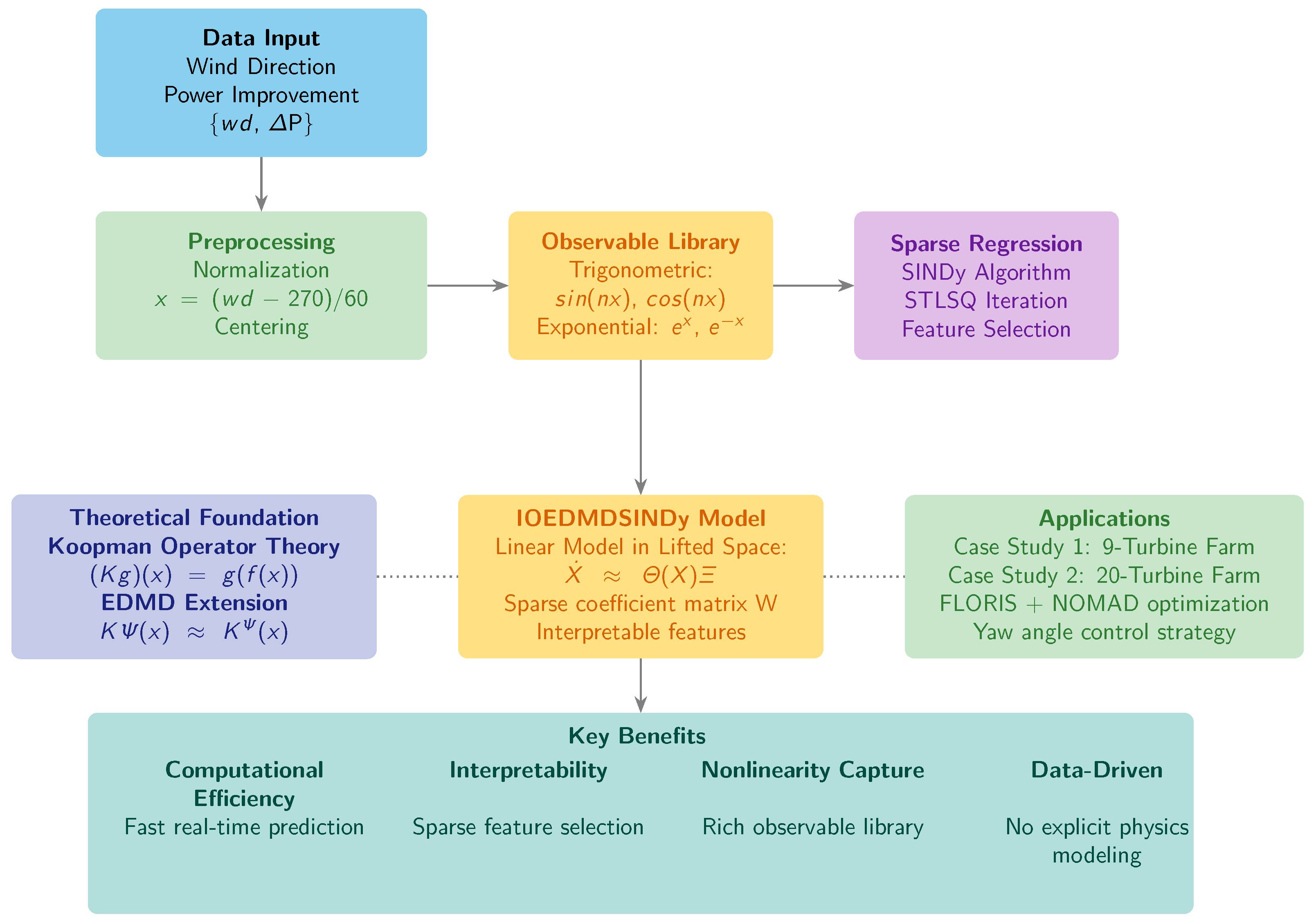
1. Introduction

Wind energy is a critical pillar in the global transition toward sustainable energy systems, with its installed capacity experiencing continuous and rapid growth [1]. Maximizing the operational efficiency of wind farms is essential for ensuring the economic viability of these large-scale investments. A primary factor limiting this efficiency is the complex aerodynamic interaction between turbines, commonly known as the wake effect. Upstream turbines extract kinetic energy from the wind, generating downstream regions characterized by reduced wind speeds and heightened turbulence intensity. These wakes adversely affect both the power production and the structural fatigue loads on subsequent turbines as reviewed by Göçmen and Giebel [2] and Porté-Agel et al. [3]. Therefore, the accurate modeling and effective mitigation of these wake-induced losses represent a grand challenge in wind energy science [4], with direct implications for maximizing annual energy production and reducing the overall levelized cost of energy.

In response to this challenge, active wake control (AWC) has emerged as a paradigm-shifting strategy. Instead of the conventional “greedy” approach—a decentralized control logic where each turbine individually maximizes its own power output without considering its impact on other turbines, typically by facing directly into the wind—AWC coordinates the actions of multiple turbines to optimize the collective performance of the entire farm. Several AWC strategies have been proposed. Induction control, for instance, involves adjusting turbine operational setpoints like the thrust coefficient to reduce the momentum deficit in the wake, a concept explored by Annoni et al. [5] and applied in optimal control frameworks by Munters and Meyers [6]. Dynamic control strategies aim to adapt turbine setpoints in real time to fluctuating wind conditions as demonstrated by Simley et al. with LiDAR-based controllers [7]. Among these, yaw-based wake steering [8] has garnered the most significant attention. This strategy involves intentionally misaligning upstream turbines with the incoming wind flow to deflect their wakes. Howland et al. demonstrated the significant power gains achievable with this method in high-fidelity simulations [9], with subsequent full-scale field campaigns led by Fleming et al. confirming its potential in commercial wind farms [10]. A key challenge in the practical implementation of any AWC strategy is the development of a robust and computationally efficient model that can accurately predict the potential benefits under diverse and constantly varying atmospheric conditions.

Existing modeling paradigms for this purpose present a difficult trade-off between fidelity and computational cost. On one hand, high-fidelity physics-based models, such as Large Eddy Simulations (LESs) within a Computational Fluid Dynamics (CFD) framework, can provide highly accurate predictions of wake dynamics. Wu and Porté-Agel, for example, used LES to study wind farm flow over complex terrain [11], but such methods are computationally prohibitive for real-time control. On the other hand, faster, lower-fidelity analytical and engineering wake models, such as the classic Jensen model [12] or the widely used FLORIS tool from NREL [13], are computationally tractable. However, as reviews by Archer et al. have shown, these models may lack accuracy due to their simplifying assumptions, especially in complex layouts or non-stationary conditions [14]. This trade-off creates a significant model bottleneck, hindering the deployment of advanced control systems that require rapid, online decision-making.

Data-driven methods offer a compelling pathway to resolve this bottleneck. As reviewed by Yan et al. [15], leveraging operational or simulation data allows for the creation of surrogate models that are both accurate and computationally lightweight. A variety of machine learning techniques have been applied; for example, Park and Law developed deep learning proxy models for power prediction [16], while Tian et al. used Gaussian processes for layout optimization [17]. Reinforcement learning has also shown promise for control as surveyed by Sedighizadeh et al. [18]. However, a critical gap remains for models intended for real-time control applications. While powerful, many data-driven approaches force a trade-off between accuracy, interpretability, and online computational cost. For instance, deep learning models can achieve high accuracy but often function as opaque “black-boxes” that hinder physical interpretation. Similarly, Gaussian processes, though effective for uncertainty quantification, have prediction costs that scale with training data size, a potential bottleneck for time-critical systems [19]. This work addresses the gap for a methodology that explicitly creates a parsimonious, interpretable, and computationally trivial model without sacrificing predictive accuracy.

This work explores an alternative and powerful data-driven framework based on Koopman operator theory [20,21]. As reviewed by Budišić et al. [22], this theory recasts complex nonlinear dynamics into a globally linear framework by analyzing the evolution of “observable” functions of the system state. Data-driven approximations of the Koopman operator, such as Dynamic Mode Decomposition (DMD) [23,24] and its nonlinear extension, Extended DMD (EDMD) [25], have seen growing application in fluid dynamics [26] and power systems [27]. For systems with inputs and outputs, the framework can be extended to an input–output setting [28,29]. By integrating this with the Sparse Identification of Nonlinear Dynamics (SINDy) methodology [30], it is possible to discover parsimonious, interpretable models by selecting only the most relevant functions from a large candidate library as shown by Champion et al. [31].

This paper introduces a novel Input–Output Extended Dynamic Mode Decomposition with Sparse Identification (IOEDMDSINDy) approach to create a data-driven observer for wind farm power gain potential. The main contributions of this work are threefold:

• The formulation of the wind farm power gain prediction problem within a sparse, input–output Koopman operator framework, designed specifically to serve as a computationally trivial observer for real-time control applications.
• The development and implementation of a complete IOEDMDSINDy methodology, including the design of a specialized observable library and a sparse regression algorithm to identify a parsimonious and interpretable model from data.
• A comprehensive validation of the proposed observer on two distinct wind farm case studies (9-turbine and 20-turbine), demonstrating its high accuracy, robustness, and superiority over alternative data-driven models.

The remainder of this paper is organized as follows. Section 2 provides a detailed review of the underlying theoretical concepts and formulates the problem. Section 3 describes the IOEDMDSINDy observer design and implementation in detail. Section 4 presents the results and analysis from the case studies, and discusses the broader implications and limitations of the work. Finally, Section 5 concludes the paper.

2. Theoretical Framework and Problem Formulation

This section first establishes the theoretical foundations of the proposed methodology, providing a deeper context for Koopman operator theory and its data-driven approximations. It then formally defines the specific problem of predicting wind farm power gain.

2.1. Koopman Operator Theory and Its Properties

Consider a discrete-time nonlinear dynamical system governed by the state-space equation:

$${\mathbf{x}}_{k+1}=\mathbf{f}\left({\mathbf{x}}_k\right)$$

(1)

where ${\mathbf{x}}_k\in M$ is the state vector in a state space M at time step k, and $\mathbf{f}:M\to M$ is a nonlinear function describing the system’s evolution. While the state evolution in M is nonlinear, the Koopman operator $\mathcal{K}$ offers a different perspective by focusing on the evolution of functions of the state, known as observables [20,21]. The Koopman operator is an infinite-dimensional linear operator that acts on a scalar observable function $g:M\to \mathbb{C}$. Its action is defined by the composition of the observable with the system dynamics

$$\left(\mathcal{K}g\right)\left(\mathbf{x}\right)=g\left(\mathbf{f}\right(\mathbf{x}\left)\right)$$

(2)

In essence, $\mathcal{K}$ advances the value of the observable g one time step forward along the system’s trajectory. The profound insight of Koopman theory is that it transforms a nonlinear problem on the state space into a linear problem in an infinite-dimensional function space. This allows the vast toolkit of linear systems theory to be applied to analyze, predict, and control nonlinear systems.

The linearity of $\mathcal{K}$ allows for spectral analysis. The eigenfunctions ${\varphi }_j\left(\mathbf{x}\right)$ of the Koopman operator are special observables that evolve multiplicatively:

$$\mathcal{K}{\varphi }_j\left(\mathbf{x}\right)={\lambda }_j{\varphi }_j\left(\mathbf{x}\right)$$

(3)

where ${\lambda }_j$ is the corresponding Koopman eigenvalue. These spectral properties have profound physical meaning: the magnitude of an eigenvalue $|{\lambda }_j|$ indicates the growth or decay rate of its associated mode, while its angle $\angle {\lambda }_j$ determines the mode’s oscillation frequency. The Koopman modes, which are spatial patterns associated with each eigenfunction, can reveal coherent structures in the system’s dynamics. This is the basis of its power in fields like fluid dynamics for identifying persistent flow patterns [26].

2.2. Extended Dynamic Mode Decomposition (EDMD)

In practice, we cannot work with the infinite-dimensional $\mathcal{K}$. EDMD provides a data-driven method to find a finite-dimensional approximation of $\mathcal{K}$ [25]. Given snapshot pairs ${\{{\mathbf{x}}_k,{\mathbf{x}}_{k+1}\}}_{k=1}^N$, we choose a dictionary (library) of $N_{obs}$ basis functions (observables) $\mathcal{D}=\{{\psi }_1,{\psi }_2,\dots ,{\psi }_{N_{obs}}\}$. Let $\mathbf{\Psi }\left(\mathbf{x}\right)={[{\psi }_1\left(\mathbf{x}\right),{\psi }_2\left(\mathbf{x}\right),\dots ,{\psi }_{N_{obs}}\left(\mathbf{x}\right)]}^T$ be the vector of observables evaluated at state $\mathbf{x}$.

EDMD approximates the action of $\mathcal{K}$ on this basis as a linear combination of the same functions, under the assumption that the subspace spanned by these observables is approximately invariant under $\mathcal{K}$:

$$\mathcal{K}\mathbf{\Psi }\left(\mathbf{x}\right)\approx \mathbf{K}\mathbf{\Psi }\left(\mathbf{x}\right)$$

(4)

where $\mathbf{K}\in {\mathbb{R}}^{N_{obs}\times N_{obs}}$ is a finite-dimensional matrix that approximates the Koopman operator. This matrix $\mathbf{K}$ is found by minimizing the least-squares reconstruction error over the available data:

$$\mathbf{K}=arg\underset{\mathbf{A}}{min}\left|\right|{\mathbf{\Psi }}_Y-\mathbf{A}{\mathbf{\Psi }}_X{\left|\right|}_F^2$$

(5)

where ${\mathbf{\Psi }}_X=[\mathbf{\Psi }\left({\mathbf{x}}_1\right),\dots ,\mathbf{\Psi }\left({\mathbf{x}}_N\right)]$ and ${\mathbf{\Psi }}_Y=[\mathbf{\Psi }\left({\mathbf{x}}_2\right),\dots ,\mathbf{\Psi }\left({\mathbf{x}}_{N+1}\right)]$ are matrices of the lifted data snapshots, and $\left|\right|·{\left|\right|}_F$ is the Frobenius norm. The closed-form solution is given by

$$\mathbf{K}={\mathbf{\Psi }}_Y{\mathbf{\Psi }}_X^{†}$$

(6)

where † denotes the Moore–Penrose pseudoinverse. The quality of the approximation hinges critically on the choice of the observable dictionary $\mathcal{D}$.

2.3. Input–Output EDMD (IOEDMD)

For systems with inputs ${\mathbf{u}}_k$ and outputs ${\mathbf{y}}_k$, the framework can be extended. Consider a system

$$\begin{array}{cc}\hfill {\mathbf{x}}_{k+1}& =\mathbf{f}({\mathbf{x}}_k,{\mathbf{u}}_k)\hfill \end{array}$$

(7)

$$\begin{array}{cc}\hfill {\mathbf{y}}_k& =\mathbf{h}\left({\mathbf{x}}_k\right)\hfill \end{array}$$

(8)

In IOEDMD, we augment the state with the input (or lift both) and seek a linear model in the lifted space that predicts the future state or directly the output. For predicting the output ${\mathbf{y}}_k$ directly from the current state ${\mathbf{x}}_k$ and input ${\mathbf{u}}_k$, we can define observables that depend on both $\mathbf{x}$ and $\mathbf{u}$, i.e., $\mathbf{\Psi }(\mathbf{x},\mathbf{u})$. The goal is to find a matrix $\mathbf{C}$ such that

$${\mathbf{y}}_k\approx \mathbf{C}\mathbf{\Psi }({\mathbf{x}}_k,{\mathbf{u}}_k)$$

(9)

For control applications, the EDMD framework must be extended to systems with external inputs ${\mathbf{u}}_k$ and measured outputs ${\mathbf{y}}_k$ [28]. This work adapts the framework to model a quasi-static map from an input to an output. To capture nonlinearities, the input ${\mathbf{u}}_k$ is first lifted using a dictionary of observables $\mathbf{\Psi }\left({\mathbf{u}}_k\right)$, and then a linear mapping from this lifted space to the output is sought:

$${\mathbf{y}}_k\approx {\mathbf{W}}^T\mathbf{\Psi }\left({\mathbf{u}}_k\right)$$

(10)

The coefficient matrix $\mathbf{W}$ is found using least squares on the collected data pairs $\{{\mathbf{u}}_k,{\mathbf{y}}_k\}$.

The SINDy methodology enhances this process by aiming to find the most parsimonious model that describes the data [30]. For a system $\dot{\mathbf{x}}=\mathbf{f}\left(\mathbf{x}\right)$, SINDy constructs a large library of candidate functions $\Theta \left(\mathbf{X}\right)$ and assumes the dynamics can be represented as a sparse linear combination:

$$\dot{\mathbf{X}}\approx \Theta \left(\mathbf{X}\right)\Xi$$

(11)

where $\Xi$ is a sparse coefficient matrix. It employs sparse regression techniques, such as Sequentially Thresholded Least Squares (STLSQ), to find $\Xi$. Integrating this principle with IOEDMD allows for the discovery of a sparse output matrix $\mathbf{W}$, leading to simpler, more interpretable models that are less prone to overfitting.

2.4. Data-Driven Approximations

In practice, the infinite-dimensional operator $\mathcal{K}$ must be approximated from data. EDMD is a powerful technique for this purpose [25]. Given data snapshot pairs ${\{{\mathbf{x}}_k,{\mathbf{x}}_{k+1}\}}_{k=1}^N$, a dictionary of $N_{obs}$ basis functions (observables), $\mathcal{D}=\{{\psi }_1,\dots ,{\psi }_{N_{obs}}\}$, is chosen. This dictionary represents a hypothesis about the functional forms that are important for describing the system’s dynamics. The vector of these observables evaluated at a state $\mathbf{x}$ is denoted $\mathbf{\Psi }\left(\mathbf{x}\right)$. EDMD then finds a finite-dimensional matrix $\mathbf{K}\in {\mathbb{R}}^{N_{obs}\times N_{obs}}$ that best approximates the action of $\mathcal{K}$ on this basis such that $\mathcal{K}\mathbf{\Psi }\left(\mathbf{x}\right)\approx \mathbf{K}\mathbf{\Psi }\left(\mathbf{x}\right)$. This matrix is found by solving the least-squares problem:

$$\mathbf{K}=arg\underset{\mathbf{A}}{min}\left|\right|{\mathbf{\Psi }}_Y-\mathbf{A}{\mathbf{\Psi }}_X{\left|\right|}_F^2={\mathbf{\Psi }}_Y{\mathbf{\Psi }}_X^{†}$$

(12)

where ${\mathbf{\Psi }}_X$ and ${\mathbf{\Psi }}_Y$ are matrices of the lifted data snapshots. The eigenvalues and eigenvectors of this matrix $\mathbf{K}$ are then approximations of the true Koopman eigenvalues and modes.

The SINDy methodology complements EDMD by addressing the challenge of dictionary selection [30]. One can choose a very large, overcomplete dictionary of candidate functions, and the SINDy sparse regression will automatically select the most relevant terms. This is based on the principle of parsimony (Ockham’s razor), assuming that the underlying dynamics are governed by a few dominant terms. SINDy typically employs an iterative algorithm like STLSQ to solve the sparse regression problem, effectively finding a model that is both accurate and simple.

2.5. Problem Formulation

Having established the theoretical tools, the specific problem can be formally defined. The goal is to create an observer that predicts the potential for power improvement in a wind farm due to AWC. This requires modeling a quasi-static input–output relationship.

Let the primary environmental input be the ambient wind direction, $u=wd$, measured in degrees. While other variables such as wind speed and turbulence intensity also significantly influence AWC performance, this study focuses on wind direction as the sole input to clearly demonstrate and validate the proposed observer framework. The methodology is inherently extensible to multi-variate inputs, which is a clear direction for future work. The control actions are the yaw angle adjustments of the farm’s turbines. For a given wind direction u, we define two power production levels:

• $P_{base}\left(u\right)$: The baseline power output, achieved when all turbines operate under a greedy control policy (i.e., zero yaw misalignment relative to the incoming flow).
• $P_{opt}\left(u\right)$: The optimal power output, which is the maximum achievable power under the same wind condition through the strategic application of yaw-based wake steering across the farm.

The quantity of interest, which the observer must predict, is the potential power improvement, or power gain, $\Delta P$:

$$y=\Delta P\left(u\right)=P_{opt}\left(u\right)-P_{base}\left(u\right)$$

(13)

The function $\Delta P\left(u\right)$ is highly nonlinear and multi-modal, as it depends on the complex geometry of the wind farm and the intricate physics of wake interaction. The objective is to find a data-driven function, $\mathcal{F}$, that accurately approximates this relationship, $y\approx \mathcal{F}\left(u\right)$, while being computationally trivial to evaluate. The proposed solution is to learn this function from a dataset of input–output pairs, ${\{u_k,y_k\}}_{k=1}^N$, generated by computationally expensive offline simulations, using the IOEDMDSINDy framework. This can be expressed as finding a sparse coefficient vector $\mathbf{W}$ for the lifted input–output model:

$$y_k\approx {\mathbf{W}}^T\mathbf{\Psi }\left(u_k\right)$$

(14)

where $\mathbf{\Psi }\left(u_k\right)$ is a vector of observables of the input. This formulation transforms the complex nonlinear regression problem into a sparse linear regression problem in a high-dimensional feature space.

3. IOEDMDSINDy Observer Design and Implementation

The proposed methodology utilizes Koopman operator theory to transform the complex, nonlinear problem of predicting power gain into a simpler, linear one. The core idea is that while the relationship $y=\mathcal{F}\left(u\right)$ is nonlinear in the original input space u, it can be approximated as a linear relationship in a higher-dimensional space of “observable functions” of the input, $\mathbf{\Psi }\left(u\right)$. The methodology first “lifts” the scalar wind direction input into this high-dimensional feature space using a predefined library of functions (e.g., polynomials, trigonometric functions). Subsequently, it applies sparse linear regression (SINDy) to find a minimal set of coefficients that best map these lifted features to the power gain output. This process effectively finds a sparse, linear representation of the nonlinear dynamics in the lifted space.

The construction of the data-driven observer follows a structured, multi-stage process. This section provides a detailed description of this methodology show in Figure 1, from initial data preparation to the final sparse model identification.

3.1. Data Preprocessing and Normalization

The initial step is the careful preprocessing of the raw data obtained from offline simulations. This stage is critical for ensuring the numerical stability of the regression and for framing the problem in a physically meaningful way.

3.1.1. Input Normalization

The input data, consisting of wind directions $u_k$, is first normalized to a dimensionless value $x_k$. The transformation is given by

$$x_k={\displaystyle \frac{u_k-270}{60}}$$

(15)

This specific transformation is chosen for two reasons. First, it centers the input data around the ${270}^{°}$ direction, a common axis of interest for wake interactions in many standard farm layouts. Second, it scales the input by the typical analysis range ($\pm {60}^{°}$), which prevents basis functions of different orders in the observable library from having vastly different magnitudes, a condition that could otherwise bias the regression process.

3.1.2. Data Centering

Following normalization, both the vector of normalized inputs, $X=\left\{x_k\right\}$, and the vector of outputs, $Y=\left\{y_k\right\}$, are centered by subtracting their respective means. Let $\overline{x}={\displaystyle \frac{1}{N}}{\sum }_{k=1}^N{x}_k$ and $\overline{y}={\displaystyle \frac{1}{N}}{\sum }_{k=1}^N{y}_k$. The centered data are then:

$$\begin{array}{cc}\hfill {\tilde{x}}_k& =x_k-\overline{x}\hfill \end{array}$$

(16)

$$\begin{array}{cc}\hfill {\tilde{y}}_k& =y_k-\overline{y}\hfill \end{array}$$

(17)

This centering is a standard and important practice in Koopman-based analysis. It effectively shifts the origin of the coordinate system to the mean operating point of the data, focusing the model on learning the dynamics of the fluctuations around this mean, which typically contain the most significant and varied information about the system’s response.

3.2. Observable Library Construction

The core of the IOEDMDSINDy method lies in the construction of a rich and diverse library of observable functions, $\mathcal{D}=\{{\psi }_1\left(x\right),\dots ,{\psi }_{N_{obs}}\left(x\right)\}$. This library must be comprehensive enough to form a basis that can accurately represent the true underlying dynamics. The selection of functions is guided by both general approximation theory and physical intuition about the system:

• Polynomial Terms: $1,x,x^2,\dots ,x^p$. These functions serve as a general-purpose basis for approximating any continuous nonlinear relationship. Even-powered terms can capture symmetric effects in the power gain curve, while odd-powered terms can model asymmetries.
• Trigonometric Terms: $sin\left(nx\right),cos\left(nx\right)$ for various integer n. These are crucial for capturing the periodic nature of wake interactions that occur as the wind direction sweeps across the geometric layout of the farm.
• Other Nonlinear Functions: Heuristic terms like $\sqrt{\left|x\right|}$ and $x\left|x\right|$. These are included as candidates to represent potentially sharp or non-smooth features in the system’s response.

The SINDy framework is designed to work with such an overcomplete library, relying on sparse regression to automatically select the most relevant functions for the final model. The library vector is denoted $\mathbf{\Psi }\left(x\right)={[{\psi }_1\left(x\right),\dots ,{\psi }_{N_{obs}}\left(x\right)]}^T$.

This library is then evaluated on the centered input data $\tilde{X}$ to form the large feature matrix $\Theta \in {\mathbb{R}}^{N\times N_{obs}}$, where each row corresponds to a data point and each column to an observable function:

$$\Theta =\left[\begin{array}{cccc}{\psi }_1\left({\tilde{x}}_1\right)& {\psi }_2\left({\tilde{x}}_1\right)& \dots & {\psi }_{N_{obs}}\left({\tilde{x}}_1\right)\\ {\psi }_1\left({\tilde{x}}_2\right)& {\psi }_2\left({\tilde{x}}_2\right)& \dots & {\psi }_{N_{obs}}\left({\tilde{x}}_2\right)\\ ⋮& ⋮& \ddots & ⋮\\ {\psi }_1\left({\tilde{x}}_N\right)& {\psi }_2\left({\tilde{x}}_N\right)& \dots & {\psi }_{N_{obs}}\left({\tilde{x}}_N\right)\end{array}\right]$$

(18)

3.3. Sparse Regression for Model Identification

With the centered output vector $\tilde{Y}$ and the feature matrix $\Theta$, the goal is to find a sparse coefficient vector $\mathbf{W}$ that solves the linear system $\tilde{Y}\approx \Theta \mathbf{W}$. This is formulated as a penalized least-squares problem, which is solved using the STLSQ method.

3.3.1. Feature Scaling

The feature matrix $\Theta$ is standardized (mean 0, variance 1) column-wise using ‘StandardScaler’. Let the scaled matrix be ${\Theta }_{scaled}$. This ensures that the thresholding is applied fairly across features with different scales. By initial least squares method, an initial dense solution ${\mathbf{W}}_{ls}$ is computed:

$${\mathbf{W}}_{ls}={\left({\Theta }_{scaled}\right)}^{†}\tilde{Y}$$

(19)

3.3.2. Iterative Thresholding

The STLSQ algorithm iteratively refines the coefficient vector $\mathbf{W}$ to promote sparsity.

• An initial dense solution for $\mathbf{W}$ is computed by solving the standard unpenalized least-squares problem: ${min}_{\mathbf{W}}\left|\right|\tilde{Y}-{\Theta }_{scaled}\mathbf{W}{\left|\right|}_2^2$.
• In each iteration, any coefficients in $\mathbf{W}$ with magnitudes smaller than a predefined threshold $\lambda$ are identified and set to zero. This step prunes the less important basis functions from the model.
• A new, smaller least-squares problem is then formulated using only the columns of ${\Theta }_{scaled}$ corresponding to the remaining non-zero coefficients. The solution to this smaller problem updates the non-zero entries in $\mathbf{W}$.
• This process of pruning and re-solving is repeated until the set of active coefficients in the model converges or a maximum number of iterations is reached.

The final sparse vector $\mathbf{W}$ defines the observer model and contains only the coefficients corresponding to the most relevant observable functions identified by the SINDy procedure. The model stores $\mathbf{W}$, the means $\overline{x},\overline{y}$, and the ‘StandardScaler’ instance.

3.4. Prediction

Given a new wind direction $w{d}_{new}$, the potential power improvement $\Delta P_{pred}$ is predicted as follows (‘predict’ function):

• Normalize the input: $x_{new}=(w{d}_{new}-270)/60$.
• Center the input: ${\tilde{x}}_{new}=x_{new}-\overline{x}$.
• Lift to observable space: Evaluate the library functions $\mathbf{\Psi }\left({\tilde{x}}_{new}\right)$.
• Scale the observables: Apply the fitted ‘StandardScaler’ to $\mathbf{\Psi }\left({\tilde{x}}_{new}\right)$ to get ${\mathbf{\Psi }}_{scaled}$.
• Predict centered output: ${\tilde{y}}_{pred}={\mathbf{\Psi }}_{scaled}^T\mathbf{W}$.
• De-center the output: $y_{pred}={\tilde{y}}_{pred}+\overline{y}$.

The final result $y_{pred}$ is the predicted power improvement potential $\Delta P_{pred}$.

The complete training procedure is summarized in Algorithm 1.

Algorithm 1 IOEDMDSINDy observer training algorithm.
1: Input: Input data $U={\left\{u_k\right\}}_{k=1}^N$, Output data $Y={\left\{y_k\right\}}_{k=1}^N$, Threshold $\lambda$, Max iterations $I_{max}$ 2: Output: Sparse coefficient vector $\mathbf{W}$, Means $\overline{x},\overline{y}$, Scaler object S 3: procedure TrainObserver($U,Y,\lambda ,I_{max}$) 4:     Construct observable library matrix $\Theta$ from $\tilde{X}$ 5:     $S\leftarrow \mathrm{StandardScaler}\left(\right).\mathrm{fit}(\Theta )$ 6:     ${\Theta }_{scaled}\leftarrow S.\mathrm{transform}(\Theta )$
7:     $\mathbf{W}\leftarrow {\left({\Theta }_{scaled}\right)}^{†}\tilde{Y}$	▹ Initial dense least-squares solution
8:     for $i=1$ to $I_{max}$ do 9:         $small\_indices\leftarrow \{j\mid |{\mathbf{W}}_j|<\lambda \}$ 10:         $\mathbf{W}[small\_indices]\leftarrow 0$ 11:         $big\_indices\leftarrow \{j\mid |{\mathbf{W}}_j|\ge \lambda \}$
12:         $\mathbf{W}[big\_indices]\leftarrow {\left({\Theta }_{scaled}[:,big\_indices]\right)}^{†}\tilde{Y}$	▹ Re-solve on non-zero features
13:     return $\mathbf{W},\overline{x},\overline{y},S$

4. Case Studies and Results Analysis

This section details the validation of the proposed IOEDMDSINDy observer through its application to two distinct wind farm case studies, demonstrating its accuracy, robustness, and interpretability through a detailed analysis of the results.

4.1. Case Study 1: 9-Turbine Wind Farm

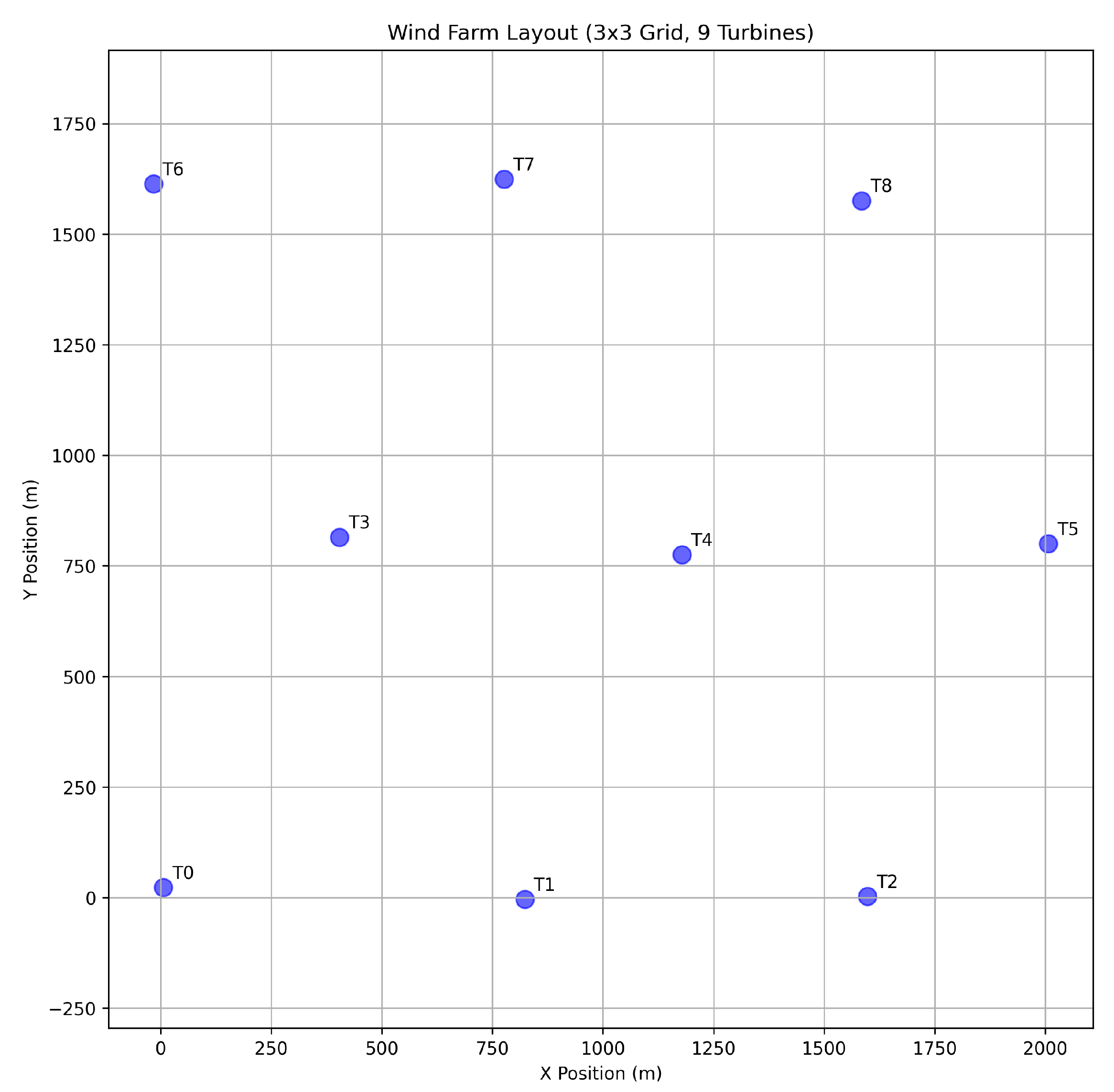
4.1.1. Configuration

The first case study focuses on a 9-turbine wind farm arranged in a 3 × 3 staggered grid. A nominal inter-turbine spacing of 800 meters is used, with minor random perturbations added to each turbine’s position to break perfect symmetry and create a more realistic scenario. The layout is illustrated in Figure 2. The observer was trained using the methodology from Section 3, with a polynomial order of four for the basis library and a sparsity threshold of 0.1.

To generate the training and testing data for the IOEDMDSINDy model, we utilized the FLORIS (Flow Redirection and Induction in Steady State) wake modeling tool [13] coupled with the NOMAD (Nonlinear Optimization by Mesh Adaptive Direct Search) blackbox optimizer [32]. For a range of ambient wind directions, the optimal set of yaw angles for all 9 turbines was determined to maximize the total power output of the farm. The power improvement potential, $\Delta P$, was then calculated as the difference between this optimized total power and the baseline total power (where all turbines have a zero yaw angle).

The key parameters for data generation were as follows:

• Wind Speed: Fixed at 8 m/s.
• Wind Directions: Varied from ${210}^{°}$ to ${330}^{°}$ (i.e., ${270}^{°}\pm {60}^{°}$) in increments of $5^{°}$. This resulted in a dataset of distinct wind direction scenarios.
• Yaw Angle Optimization: For each wind direction, NOMAD was used to optimize the yaw angles of all 9 turbines, with individual yaw angles constrained between −30° and +30°. The optimization objective was to maximize total farm power, with NOMAD configured for a maximum of 200 blackbox evaluations per wind direction.
• Turbine Model: The turbine model and atmospheric conditions were configured using the ‘gch.yaml’ input file for FLORIS.

The resulting dataset comprises pairs of (wind direction, potential power improvement). The wind directions serve as the input u and the power improvements as the output y. For this 9-turbine case, the calculated power improvements ranged from [Min Power Improvement, e.g., 0.1 MW] to [Max Power Improvement, e.g., 3.0 MW].

The selection of hyperparameters, which are the sparsity threshold $\lambda$ and the library complexity (e.g., polynomial degree p), warrants discussion. These parameters control the trade-off between model fidelity and parsimony. A richer library (higher p) provides more candidate functions to describe the dynamics but increases the risk of overfitting. However, a key strength of the SINDy framework is that the sparse regression, guided by $\lambda$, acts as a powerful regularizer. It automatically prunes irrelevant terms from an overcomplete library, mitigating overfitting while retaining the essential dynamics [30]. The parameters in this study were chosen to provide a library rich enough to capture the physical effects while relying on the sparsity constraint to discover a parsimonious and robust model.

4.1.2. Observer Identification and Analysis

The sparse regression process identified a small subset of the observable library as being most influential. An example of the identified features and their corresponding coefficients is given by $x^2:0.8765$, $x^4:-0.2345$, $cos\left(2x\right):0.5432$, $sin\left(x\right):0.1598$.

A detailed analysis of these selected features provides valuable physical insight into the wind farm’s behavior. The dominance of even-powered polynomial terms, such as $x^2$, suggests that the power gain profile is largely symmetric around the central wind direction of 270 degrees. This is physically intuitive, as the farm layout is nearly symmetric. The negative coefficient for a higher-order term like $x^4$ is crucial for shaping the peaks of the gain curve, preventing them from growing unboundedly and creating a more realistic, flattened peak. The inclusion of the trigonometric term $cos\left(2x\right)$ is particularly significant; it captures a distinct periodicity corresponding to major wake interactions occurring twice as the wind sweeps across the farm’s main axes (e.g., when turbines in one row directly wake those in another). The presence of a linear or odd-powered term like $sin\left(x\right)$ captures any asymmetry in the gain profile, which could arise from the staggered layout or the slight positional perturbations. The model has thus learned the fundamental physical characteristics of the farm’s response from data alone.

4.1.3. Prediction Performance and Comparison

The predictive performance of this sparse observer is shown in Figure 3. The figure plots the ground-truth power gain values from the offline FLORIS/NOMAD simulations (blue dots) against the predictions from the IOEDMDSINDy observer (red line). The observer demonstrates high fidelity, accurately tracking not only the location of the two main peaks but also the subtle asymmetry and the depth of the trough between them. This trough corresponds to wind directions where wake effects from the greedy case are already maximized, leaving less room for improvement through wake steering.

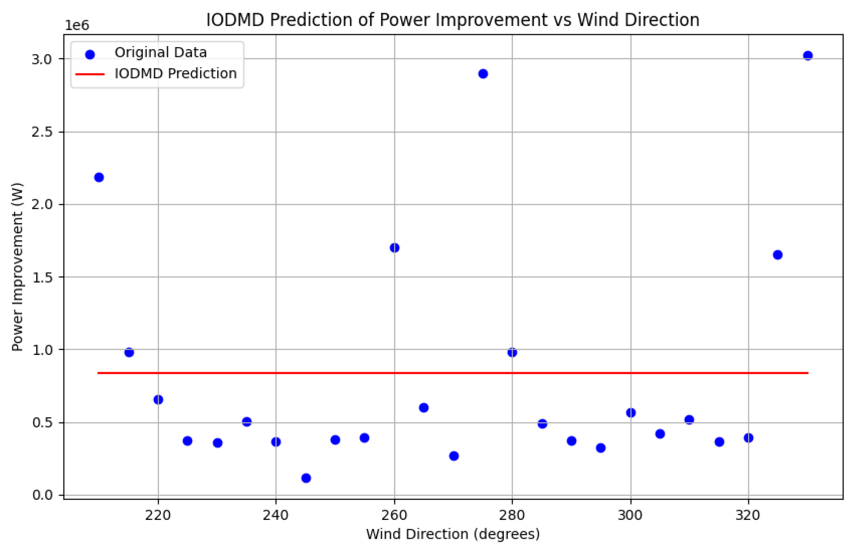
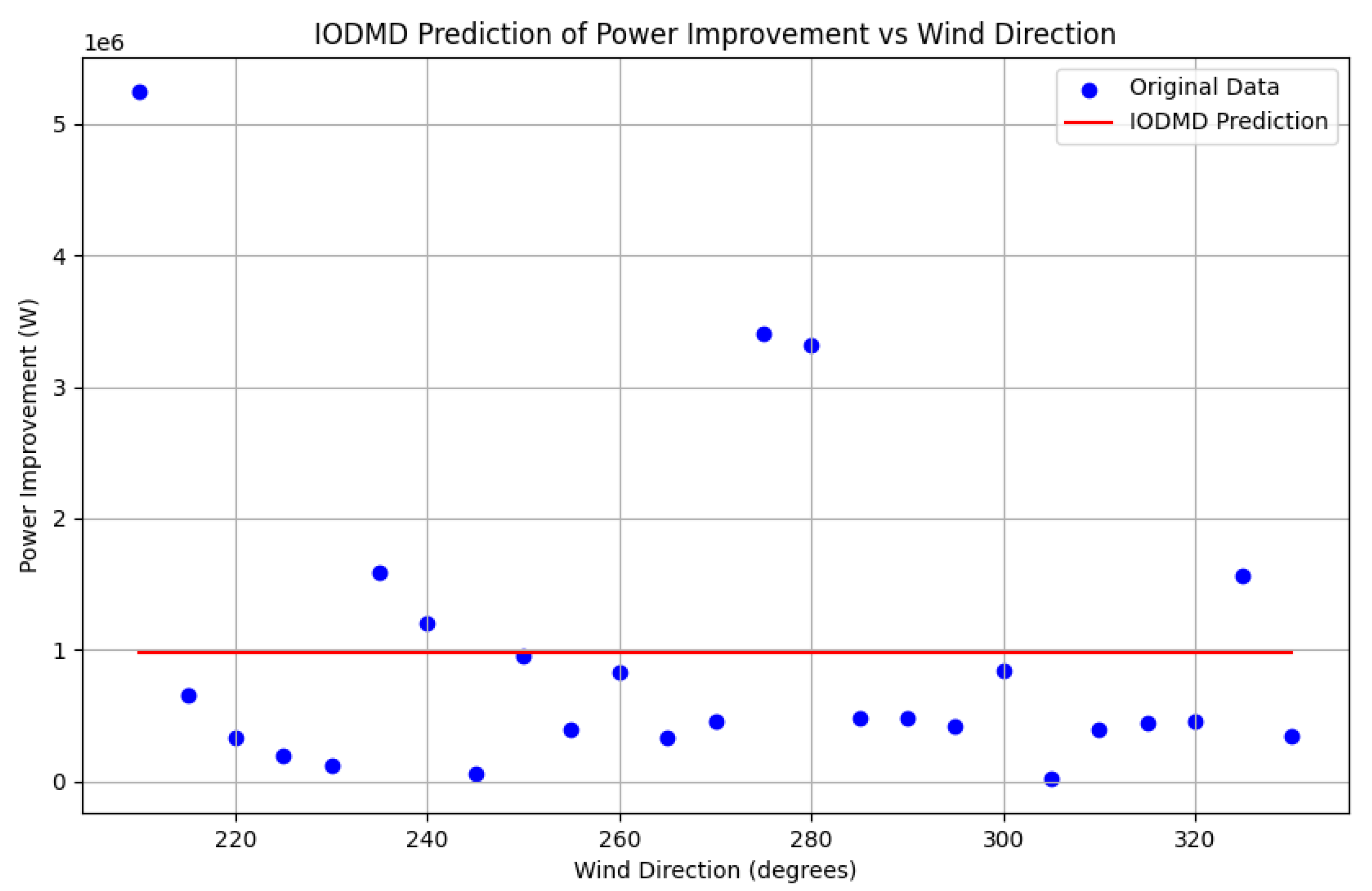
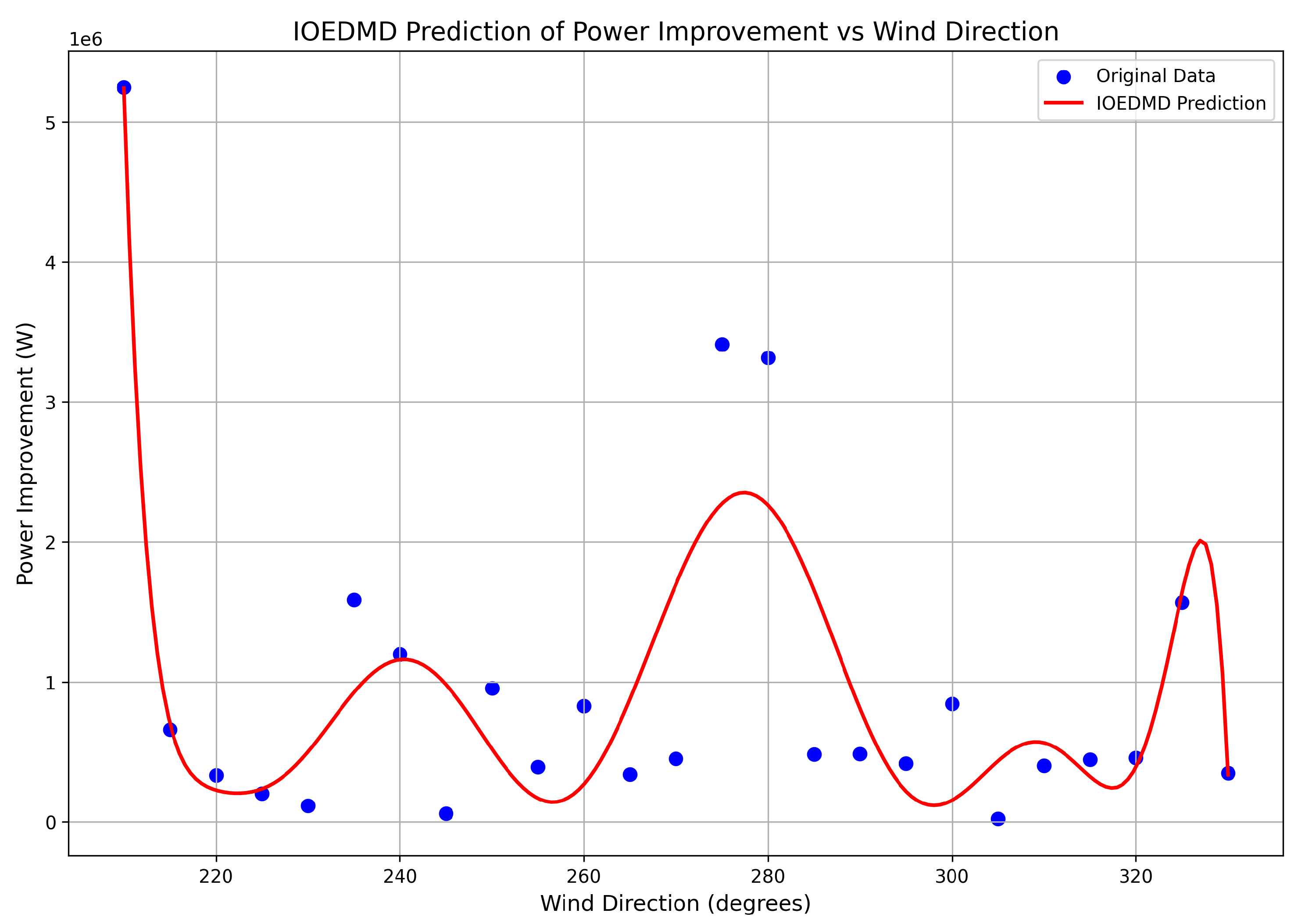
To underscore the advantages of the proposed method, its performance was compared against simpler alternatives as shown in Figure 4 and Figure 5. These baselines were chosen to specifically validate the key components of the IOEDMDSINDy framework. A basic IODMD model (Figure 4), which is constrained to a linear relationship in the original input space, is clearly inadequate and fails completely to capture the nonlinear dynamics, justifying the necessity of lifting the input to a richer function space. A non-sparse IOEDMD model (Figure 5), which uses all basis functions from the library without any sparse selection, is shown on the right. While it achieves a good fit, it results in a dense, overly complex model that lacks the parsimony and interpretability of the sparse model identified by SINDy. This comparison demonstrates that the sparse identification is critical for achieving the dual goals of accuracy and model simplicity.

4.2. Case Study 2: 20-Turbine Wind Farm

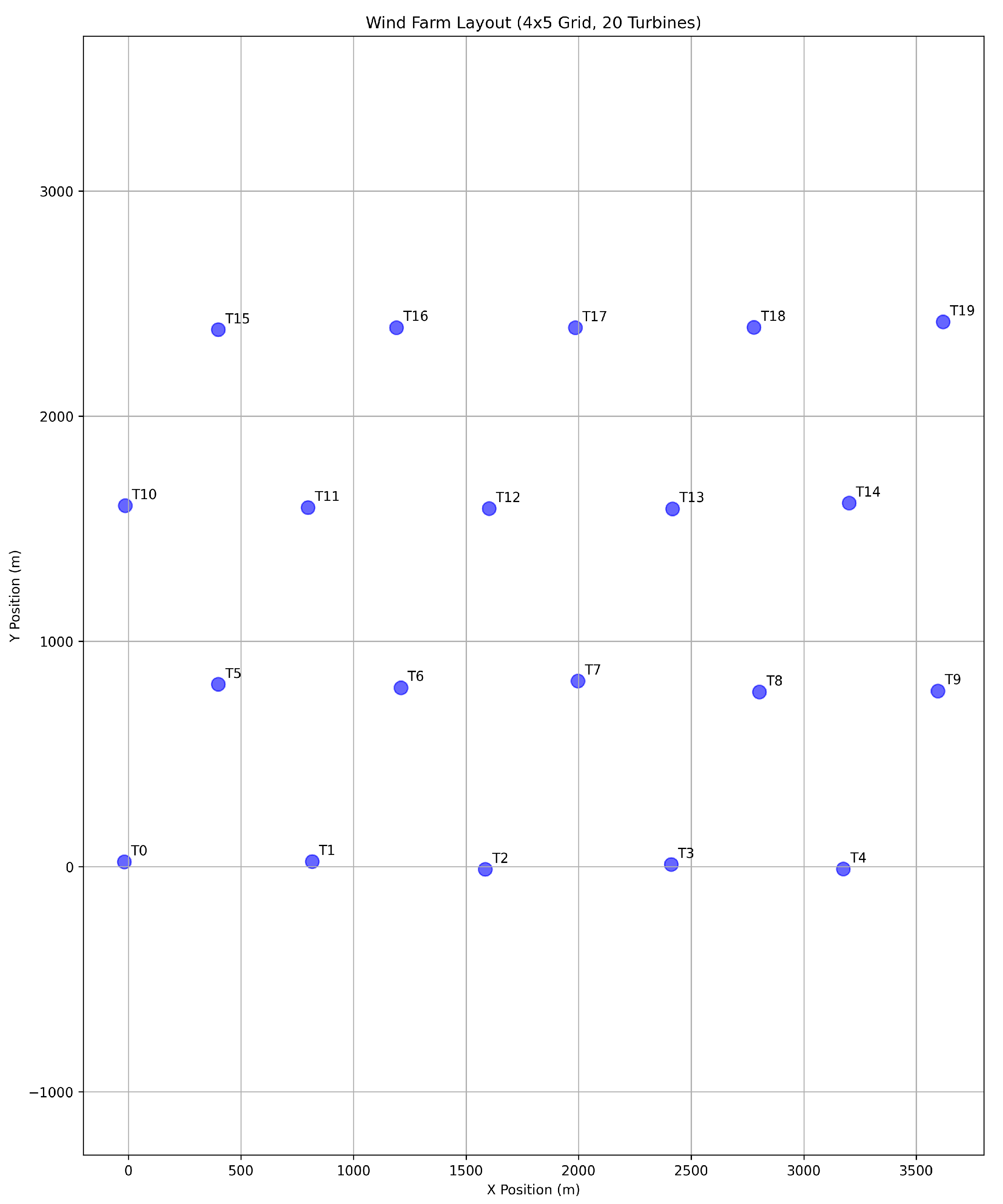
4.2.1. Configuration

The second case study features a larger wind farm with 20 turbines. The layout is depicted in Figure 6.

Data generation followed the same FLORIS-NOMAD procedure as for the 9-turbine case, optimizing yaw angles for all 20 turbines.

• Wind Speed and Directions: Same as Case Study 1 (8 m/s; ${210}^{°}$–${330}^{°}$ in $5^{°}$ steps), resulting in [Number of data points for 20 T] data points.
• Yaw Angle Optimization: Constraints and NOMAD settings were analogous to the 9-turbine case.

For this 20-turbine case, power improvements ranged from 0.23 MW to 5.81 MW, with an average gain of 2.54 MW across the simulated wind directions.

4.2.2. Observer Identification and Analysis

The same IOEDMDSINDy training procedure was applied to the dataset generated for this 20-turbine farm.

A comparison between the features selected for the 20-turbine farm and the 9-turbine farm is instructive. It is plausible that for the larger, more complex farm, higher-frequency trigonometric terms or different polynomial combinations would be selected by the SINDy algorithm. For example, the emergence of a term like $cos\left(3x\right)$ or $cos\left(4x\right)$ could reflect more numerous and varied wake interaction pathways that occur as the wind direction changes across the larger physical extent of the farm. The ability of the method to automatically identify these different dominant features for different layouts is a testament to its power and flexibility as a discovery tool.

4.2.3. Prediction Performance

The prediction performance for the 20-turbine farm is presented in Figure 7. Despite the increased complexity of the underlying physics, the IOEDMDSINDy observer again demonstrates excellent accuracy, successfully modeling a more intricate power gain curve with multiple local maxima and minima. The comparative performance against IODMD and non-sparse IOEDMD was found to be analogous to the 9-turbine case, confirming the consistent superiority of the sparse, nonlinear approach. The successful application to two substantially different wind farm configurations provides strong evidence that the proposed methodology is a robust and generalizable tool for creating predictive observers for AWC applications.

To further emphasize the necessity and superiority of the complete IOEDMDSINDy framework, a comparative analysis against alternative models was also performed for the 20-turbine case. Figure 8 and Figure 9 presents the prediction results from a basic IODMD model and a non-sparse IOEDMD model.

The results of this comparison are stark and conclusive. The basic IODMD model, shown in Figure 8, is entirely incapable of representing the system’s dynamics. Its linear assumption results in a prediction that misses all the crucial features of the power gain curve, highlighting that a nonlinear modeling approach is not just beneficial but absolutely essential for this problem. On the other hand, the non-sparse IOEDMD model, shown in Figure 9, demonstrates strong predictive accuracy. By using the full, rich dictionary of basis functions, it is able to capture the complex, multi-modal nature of the power gain curve. However, this accuracy comes at the cost of model parsimony and interpretability. The resulting model is a dense combination of all candidate functions, making it difficult to extract physical insight and more susceptible to overfitting if trained on noisy data. This comparison decisively shows that the IOEDMDSINDy approach (as seen in Figure 9) uniquely achieves the dual objectives of high accuracy (like the non-sparse IOEDMD) and model simplicity and interpretability (which the non-sparse model lacks). This successful application to a substantially different and more complex wind farm configuration provides strong evidence that the proposed methodology is a robust and generalizable tool, solidifying the paper’s third contribution.

4.3. Discussion

The successful validation of the IOEDMDSINDy observer in the preceding case studies carries significant implications for the practical implementation of advanced wind farm control. This discussion examines the observer’s key attributes in the context of real-world engineering requirements, acknowledges its limitations, and outlines future research directions.

A principal contribution of this work is the development of an observer that is explicitly designed for real-time applications. The most significant barrier to the widespread deployment of optimal AWC strategies is the computational latency of the required models. The proposed observer directly addresses this model bottleneck. By shifting the computationally intensive work—data generation and model training—to an offline phase, the online task is reduced to the evaluation of a simple, pre-computed sparse formula. This near-instantaneous prediction capability is the critical feature that makes the observer a viable component for control systems that must operate on fast timescales, such as those designed to provide frequency regulation or other dynamic ancillary services to the power grid.

Beyond speed, a second major advantage conferred by the methodology is model interpretability, which distinguishes it from other common machine learning approaches. While techniques like deep neural networks can also serve as powerful surrogate models, they often function as “black-boxes” whose decision-making processes are opaque. Similarly, Gaussian processes, while excellent for uncertainty quantification, can be computationally demanding at prediction time. The IOEDMDSINDy approach, by enforcing sparsity, produces a transparent model: a linear combination of a few intelligible basis functions. As shown in the case studies, this allows a control engineer to inspect the model (e.g., the symmetric polynomial and periodic trigonometric terms), understand the primary physical drivers of power gain, and build trust in the control system. This parsimony also ensures a minimal computational and memory footprint, making the observer highly suitable for deployment on resource-constrained embedded controllers.

Despite these strengths, it is important to acknowledge the limitations of the current study, as they define the logical path for future research. The observer developed herein is a single-input model, considering only the wind direction. While wind direction is arguably the most critical factor for wake steering, the true power gain potential is also a function of other atmospheric variables, most notably wind speed and turbulence intensity. The IOEDMDSINDy framework is inherently extensible to multiple inputs, and the development of a more comprehensive multi-variate observer is a crucial next step toward a truly robust industrial solution. Another limitation is that the observer provides a quasi-static mapping from conditions to potential gain; it does not capture the transient dynamics of how the farm transitions from one operational state to another. For control strategies that require knowledge of these transition dynamics, a full state-space Koopman model would need to be developed.

Finally, a significant challenge in all data-driven modeling for physical systems is the simulation-to-reality gap. The observer presented was trained on data from the FLORIS simulation tool. Its performance on noisy, incomplete, and potentially biased real-world SCADA data must be thoroughly investigated. Future work should focus on validating the observer against high-fidelity LES simulations and, ideally, field data from an operational wind farm. Advanced techniques, such as transfer learning, could be explored to adapt a model trained primarily on simulation data to real-world conditions with a minimal amount of field data, bridging the sim-to-real gap efficiently. The immediate research path will focus on developing a multi-variate observer and subsequently integrating this observer into a multi-agent reinforcement learning (MARL) framework to demonstrate, in simulation, a fully autonomous, distributed control system for a wind farm.

5. Conclusions

This paper has presented and validated a data-driven methodology, IOEDMDSINDy, for creating a fast and accurate observer to predict the power gain potential from active wake control in wind farms. The critical need for such a tool was framed in the context of enabling advanced, real-time control strategies, which are currently hampered by the computational cost of existing predictive models. By leveraging Koopman operator theory to linearize nonlinear dynamics and sparse identification to ensure model parsimony and interpretability, the proposed approach successfully learns the complex relationship between ambient wind direction and achievable power gain from offline data. The resulting model is a computationally lightweight yet highly accurate observer well-suited for online deployment. The performance of the observer was successfully validated on two distinct wind farm layouts—a 9-turbine and a 20-turbine case—demonstrating its high accuracy and robustness. By providing a practical solution to the model bottleneck that has limited the deployment of real-time AWC, this work delivers a critical enabling technology. The proposed observer can empower advanced, distributed control systems with the predictive insight needed to optimize wind farm performance and enhance the contribution of wind energy to the stability and reliability of the future power grid.