Degradation Prediction of Proton Exchange Membrane Fuel Cell Based on Multi-Head Attention Neural Network and Transformer Model

Abstract

Proton exchange membrane fuel cells are a clean energy technology with wide application in transportation and stationary energy systems. Due to the problem of voltage degradation under long-term dynamic loads, predicting their performance degradation trend is of great significance for extending the life of proton exchange membrane fuel cells and improving system reliability. This study adopts a data-driven approach to construct a degradation prediction model. In view of the problem of many input parameters and complex distribution of degradation features, a neural network model based on a multi-head attention mechanism and class token is first proposed to analyze the impact of different operating parameters on the output voltage prediction. The importance of each input variable is quantified by the attention weight matrix to assist feature screening. Subsequently, a prediction model is constructed based on Transformer to characterize the voltage degradation trend of fuel cells under dynamic conditions. The experimental results show that the root mean square error and mean absolute error of the model in the test phase are 0.008954 and 0.006590, showing strong prediction performance. Based on the importance evaluation provided by the first model, 11 key parameters were selected as inputs. After this input simplification, the model still maintained a prediction accuracy comparable to that of the full-feature model. This result verifies the effectiveness of the feature screening strategy and demonstrates its contribution to improved generalization and robustness.

1. Introduction

Energy and environmental challenges have become increasingly critical in recent years. Proton exchange membrane fuel cells (PEMFCs), as a zero-emission and efficient technology, are widely regarded as a promising solution to these issues [1,2,3]. PEMFCs are considered essential in new energy applications, with strong potential in electric vehicles, aviation, and industrial power [4,5,6]. However, the widespread adoption of PEMFCs, particularly in fuel cell electric vehicles (FCEVs), is hindered by their limited useful life and high costs [7,8,9,10]. The useful life of a PEMFC is closely related to its degradation, which affects key parameters such as voltage, efficiency, and power output [11].

The long-term operating conditions accelerate the degradation of key components within the PEMFC system; this degradation includes carbon corrosion, catalyst particle maturation, and gas diffusion layer compression [12,13]. Strahl et al. [14] investigated the relationship between degradation mechanisms and fuel cell performance loss to analyze changes in electrochemical behavior and structural characteristics during operation. Dhimish et al. [15] estimated degradation mechanisms for fuel cells operating under different operating conditions, including results for high and low temperature variations. These studies highlight that different operating conditions have a significant influence on the dominant degradation mechanisms. Therefore, accurately predicting the degradation of PEMFCs under these conditions is crucial to extending their lifetime and reducing maintenance costs [16,17].

Common methods for the degradation prediction of PEMFCs are classified into three categories: model-based, data-driven, and hybrid methods [18]. The model-based method is based on physical models or empirical models [19]. It uses equations that describe the electrochemical reactions, mass transport, and thermal behavior inside the fuel cell. These models require detailed knowledge of the system and accurate parameter identification. Mayur et al. [20] proposed a method that couples a 2D multi-physics cell model with a vehicle load model using a flexible degradation library to simulate component-wise degradation and time-upscaling techniques for predicting PEMFC aging. Pei et al. [21] proposed an empirical model based on load changing cycles, start–stop cycles, idling time, high power load condition, and the air pollution factor, which can reliably predict the lifetime of fuel cells under various operating conditions. Ou et al. [22] proposed a semi-empirical model-based prognostics method based on the polarization behavior of PEMFCs, which incorporates degradation models for electrochemical surface area and equivalent resistance. Although model-based approaches provide clear interpretability and can capture internal degradation processes, they usually involve high computational cost and complex structures. Moreover, physics-based simulations often fall short in terms of efficiency, especially for engineering applications [23].

The data-driven method relies on historical operation data of the fuel cell. It applies statistical analysis or machine learning algorithms to learn the relationship between input features and performance [24,25]. This method does not require in-depth physical understanding, making it easier to apply [26]. Chen et al. [27] proposed a method for predicting PEMFC degradation, combining multi-kernel relevance vector regression with the whale optimization algorithm. By incorporating real-world driving data and laboratory measurements, this approach creates a robust model that covers a wide range of operating conditions. Wilberforce et al. [28] used artificial neural network (ANN) and two different learning algorithms to predict the performance of PEMFCs in terms of power and voltage under various operating conditions and analyzed the relationship between voltage and operating conditions. Sahajpal et al. [29] investigated six deep learning architectures for long-term degradation prediction, including Long Short-Term Memory (LSTM), Gated Recurrent Unit (GRU), Convolutional Neural Network (CNN), and their combinations. Zuo et al. [30] focused on degradation prediction under a dynamic cycling condition and compared the prediction results using LSTM, GRU, Attention-based LSTM, and Attention-based GRU. By combining the attention mechanism with the other models, the new model has higher prediction accuracy and is more suitable for processing PEMFC dynamic test data. Yu et al. [31] delved into feature parameters, extracting underlying patterns of feature evolution. The authors then combined this approach with Mogrifier LSTM, which significantly improves the accuracy and stability of PEMFC performance degradation prediction. Li et al. [32] proposed a fusion prognostic framework based on bi-direction LSTM, bi-direction GRU, and echo state network (ESN), which can achieve short-term degradation prediction. Yang et al. [33] combined GRU with Minimal Gated Unit (MGU) and integrated it with an attention mechanism, improving the accuracy and controllability of aging prediction.

The hybrid method combines the strengths of both model-based methods and data-driven techniques [34]. This approach improves generalization, but it can be more difficult to design and tune. Pan et al. [35] proposed a hybrid approach that combines a model-based adaptive Kalman filter and a data-driven nonlinear autoregressive exogenous (NARX) model. The overall degradation trend is captured by the empirical aging model, while the NARX neural network describes the detailed degradation information. Although the hybrid method has shown potential, the underlying theoretical framework and models remain in the process of ongoing development and refinement. Additionally, challenges persist regarding the stability and accuracy of the model.

In the above works, most data-driven studies are based on LSTM, GRU, and CNN, which perform well in sequence data processing. However, they often encounter issues such as gradient vanishing or explosion when handling long sequences, leading to ineffective capture of long-term dependencies [36]. Moreover, previous studies have generally overlooked the analysis of the parameters’ importance, resulting in limited interpretability of the model. Furthermore, much of the research focuses on steady-state or quasi-steady-state loads. In contrast, real-world operating conditions of PEMFCs are more complex, necessitating research under dynamic load conditions.

To solve these problems, this study proposed two neural networks for PEMFC degradation prediction under dynamic cycling conditions. First, a multi-head attention neural network with a class token is developed. This model can effectively capture the complex relationship between input features and improve the model’s ability to focus on key features, thereby enhancing the model’s interpretability. Second, a Transformer Encoder model is introduced, which captures long-term dependencies through positional encoding, residual connections, and self-attention. Compared to traditional RNN and CNN models, the Transformer Encoder avoids gradient vanishing or explosion when processing long sequences. Additionally, it enables parallel processing of sequence data, improving computational efficiency. Based on the analysis of the multi-head attention neural network results, the most influential operational parameters for the prediction results were selected as inputs for the Transformer Encoder model. The chosen parameters generally retain the essential information of the original parameters, thereby reducing model complexity, mitigating the risk of overfitting, and enhancing the model’s generalization ability.

2. Degradation Prediction Model

Two neural network models are applied to solve the challenge of PEMFC degradation prediction. The Multi-Head Attention with Class Token Model (MHA-CLS) is used to analyze the impact of operating parameters on PEMFC performance, while the Transformer Encoder model is used for predicting the performance after the degradation of PEMFC. The fundamental theories of these models are explained, and the models are constructed.

2.1. Multi-Head Attention with Class Token Model

The idea of the attention mechanism is that when processing data, the model does not need to uniformly focus on all input information [37]. Instead, it can assign different attention weights to each input element during prediction, reflecting their importance. The class token was introduced to obtain these attention weights. Based on this principle, the impact of different operating parameters on PEMFC degradation can be obtained in the prediction process.

2.1.1. Attention Mechanism

In attention mechanisms, the input typically represents the data that is fed into the model. To compute the attention, the input is projected into three distinct vectors, query, key, and value, through linear transformations using learned weight matrices.

The query-key-value structure forms the fundamental operation of attention. The query vector interacts with the key vectors to generate attention scores, which are subsequently applied to the value vectors. The result is a weighted sum of the values, where higher attention scores correspond to more significant elements of the input. The commonly used Scaled Dot-Product Attention [38] is computed as:

$$\mathrm{A}\mathrm{t}\mathrm{t}\mathrm{e}\mathrm{n}\mathrm{t}\mathrm{i}\mathrm{o}\mathrm{n}\left(\mathrm{Q},\mathrm{K},\mathrm{V}\right)=\mathrm{s}\mathrm{o}\mathrm{f}\mathrm{t}\mathrm{m}\mathrm{a}\mathrm{x}\left({\displaystyle \frac{\mathrm{Q}{\mathrm{K}}^{\mathrm{T}}}{\sqrt{{\mathrm{d}}_{\mathrm{k}}}}}\right)\mathrm{V}$$

(1)

where Q is the matrix of queries, representing the current input that needs to attend to the other parts of the sequence. K is the matrix of keys, representing the reference or the contextual information that the model will use to compare against the queries. V is the matrix of values, containing the actual information to be weighted and aggregated based on the attention scores. ${\mathrm{d}}_{\mathrm{k}}$ is the dimension of the key vectors, and $\sqrt{{\mathrm{d}}_{\mathrm{k}}}$ is used as a scaling factor to prevent overly large dot-product values, which could result in unstable gradients. The Softmax function is used to transform the scaled dot products into a probability distribution, ensuring that the attention weights are positive and sum to 1. The schematic of the attention mechanism is shown in Figure 1.

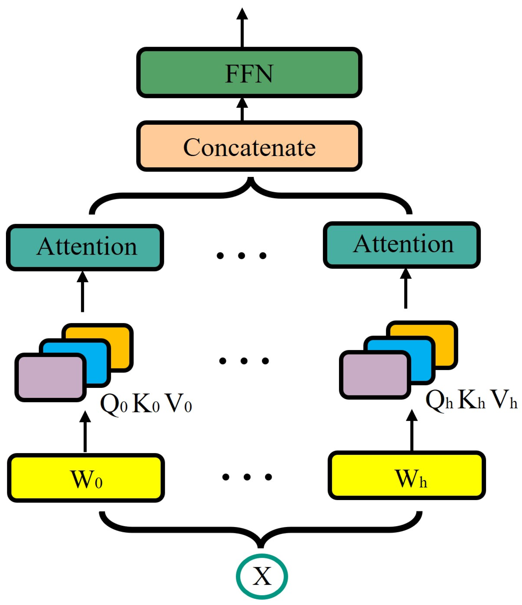
2.1.2. Multi-Head Attention with Feedforward Network

A single attention mechanism may overlook certain information. In contrast, multi-head attention (MHA) uses multiple independent attention heads to extract features from different perspectives and then combines the information, thereby enhancing the model’s representational capacity [38]. The mathematical formulation of MHA is as:

$$\mathrm{M}\mathrm{u}\mathrm{l}\mathrm{t}\mathrm{i}\mathrm{H}\mathrm{e}\mathrm{a}\mathrm{d}\left(\mathrm{Q},\mathrm{K},\mathrm{V}\right)=\mathrm{C}\mathrm{o}\mathrm{n}\mathrm{c}\mathrm{a}\mathrm{t}\left(\mathrm{A}\mathrm{t}\mathrm{t}\mathrm{e}\mathrm{n}\mathrm{t}\mathrm{i}\mathrm{o}\mathrm{n}({\mathrm{Q}}_1,{\mathrm{K}}_1,{\mathrm{V}}_1),\dots ,\mathrm{A}\mathrm{t}\mathrm{t}\mathrm{e}\mathrm{n}\mathrm{t}\mathrm{i}\mathrm{o}\mathrm{n}({\mathrm{Q}}_{\mathrm{h}},{\mathrm{K}}_{\mathrm{h}},{\mathrm{V}}_{\mathrm{h}})\right){\mathrm{W}}^{\mathrm{O}}$$

(2)

where h is the number of attention heads. Each head independently computes the attention for its respective query, key, and value vectors. The outputs of all attention heads are concatenated and then multiplied by the output weight matrix ${\mathrm{W}}^{\mathrm{O}}$, which projects the combined results into the desired output space. This allows the model to jointly attend to information from different representation subspaces, thereby enhancing its ability to capture a diverse set of features. The diagram of the MHA is presented in Figure 2.

The outputs of the MHA need to pass through a Feedforward Network (FFN), which applies non-linear transformations to further process the information. This network is composed of two fully connected layers, with a ReLU activation function applied between them. The FFN can be calculated as:

$$\mathrm{F}\mathrm{F}\mathrm{N}\left(\mathrm{x}\right)=\mathrm{m}\mathrm{a}\mathrm{x}(0,\mathrm{x}{\mathrm{W}}_1+{\mathrm{b}}_1){\mathrm{W}}_2+{\mathrm{b}}_2$$

(3)

where x is the input to the FFN, ${\mathrm{W}}_1$ and ${\mathrm{W}}_2$ are weight matrices, ${\mathrm{b}}_1$ and ${\mathrm{b}}_2$ are bias terms, and max function is the ReLU activation function. The ReLU function introduces non-linearity into the model, enabling it to capture more complex patterns and relationships within the data. The FFN enables the model to learn complex transformations of the input representations.

2.1.3. Class Token

The attention mechanism primarily measures the relationships between input features. To capture the contribution of each feature to the final prediction, the class token can be introduced. Through its attention weights, it quantifies the importance of each input feature in the prediction process. The class token originates from the Transformer architecture and is widely used in models like the Vision Transformer (ViT) [39,40,41]. In ViT, it acts as a trainable embedding that interacts with other input features, aggregating global information to enhance feature extraction.

In this study, a class token is incorporated into the multi-head attention model as a learnable parameter, initialized using a Gaussian distribution and optimized during training. It is treated as an additional input element in the attention mechanism, participating in the computation of queries, keys, and values with other input features. This design allows the class token to aggregate global information from the input operating parameters, which is processed through the linear layer for prediction, while the attention weights reflect the contribution of each input to the final output. The implementation workflow for the MHA-CLS is depicted in Figure 3.

2.2. Transformer Encoder Model

The Transformer model is a deep learning architecture based on the attention mechanism, originally designed for sequence modeling tasks [38]. Unlike other models such as RNNs or LSTMs, Transformers use self-attention mechanisms to capture relationships between distant time steps [42]. This allows it to effectively model complex temporal dependencies in time series data, regardless of how far apart the relevant data points are in the sequence. In contrast to sequential models, which process time steps one at a time, the Transformer model processes the entire sequence in parallel. This makes it significantly faster to train as it benefits from modern hardware acceleration. The Transformer model is structured with an encoder-decoder framework, where the encoder processes input sequences to extract meaningful representations, and the decoder generates sequence outputs. In this study, the focus is on predicting the performance after the degradation of PEMFC, which primarily requires the extraction of feature representations rather than sequence generation. Therefore, the Transformer Encoder model is used, as it is specifically designed to capture the necessary feature representations [43,44].

The Transformer Encoder model consists of several key components that work together to process input data and extract meaningful feature representations. In addition to the MHA and the FFN, the Transformer Encoder model also includes position encoding, layer normalization, and residual connections. A conceptual view of the standard Transformer Encoder model is shown in Figure 4.

2.2.1. Position Encoding

The Transformer Encoder model incorporates position encoding to address the lack of inherent sequential processing. Since the Transformer processes input data in parallel, position encoding is used to inject information about the relative position of tokens within the sequence. This step can be written as:

$${\mathrm{x}}_{\mathrm{t}}^{\mathrm{e}\mathrm{n}\mathrm{c}\mathrm{o}\mathrm{d}\mathrm{e}\mathrm{d}}={\mathrm{x}}_{\mathrm{t}}+{\mathrm{p}}_{\mathrm{t}} \mathrm{f}\mathrm{o}\mathrm{r} \mathrm{t}=\mathrm{1,2},\dots ,\mathrm{T}$$

(4)

where T is the number of time steps in the sequence, and ${\mathrm{p}}_{\mathrm{t}}$ represents the position encoding for the t time step. This allows the model to maintain the order of the input sequence, which is crucial for predicting PEMFC degradation over time.

2.2.2. Residual Connection and Layer Normalization

Each encoder layer consists of two main sub-layers: the MHA layer and FFN layer. Residual connections are added around both main sub-layers. These connections help to mitigate the vanishing gradient problem by allowing the gradients to flow more easily through the network during backpropagation. After each sub-layer, layer normalization is applied to stabilize the learning process and improve training efficiency by normalizing the input to each layer. These two processes can be expressed as

$$\mathrm{O}\mathrm{u}\mathrm{t}\mathrm{p}\mathrm{u}\mathrm{t}=\mathrm{L}\mathrm{a}\mathrm{y}\mathrm{e}\mathrm{r}\mathrm{N}\mathrm{o}\mathrm{r}\mathrm{m}\left(\mathrm{M}\mathrm{u}\mathrm{l}\mathrm{t}\mathrm{i}\mathrm{H}\mathrm{e}\mathrm{a}\mathrm{d}\right(\mathrm{Q},\mathrm{K},\mathrm{V})+\mathrm{X})$$

(5)

where X is the original input. The output of each encoder layer is passed through these mechanisms iteratively, with each layer refining the feature representations, ultimately capturing complex dependencies and relationships between input features.

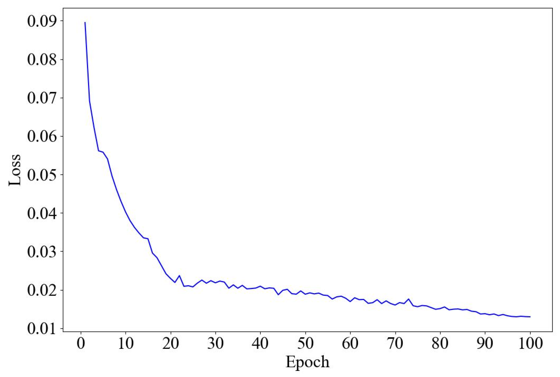
2.2.3. Training Optimization Strategies

In the training process of the Transformer model, the optimizer and regularization methods play a crucial role in improving model performance. This study applies the Adam optimizer for parameter updates and dropout for regularization to enhance training stability and prevent overfitting.

The adaptive moment estimation (Adam) optimizer combines momentum and adaptive learning rate adjustment, enabling stable convergence and avoiding local minima. The updated equations are given by:

$${\mathrm{m}}_{\mathrm{i}}={\mathsf{\beta }}_1{\mathrm{m}}_{\mathrm{i}-1}+(1-{\mathsf{\beta }}_1){\mathrm{g}}_{\mathrm{i}}$$

(6)

$${\mathrm{v}}_{\mathrm{i}}={\mathsf{\beta }}_2{\mathrm{v}}_{\mathrm{i}-1}+(1-{\mathsf{\beta }}_2){\mathrm{g}}_{\mathrm{i}}^2$$

(7)

$${\widehat{\mathrm{m}}}_{\mathrm{i}}={\displaystyle \frac{{\mathrm{m}}_{\mathrm{i}}}{1-{\mathsf{\beta }}_1^{\mathrm{i}}}},{\widehat{\mathsf{\nu }}}_{\mathrm{i}}={\displaystyle \frac{{\mathsf{\nu }}_{\mathrm{i}}}{1-{\mathsf{\beta }}_2^{\mathrm{i}}}}$$

(8)

$${\mathsf{\theta }}_{\mathrm{i}}={\mathsf{\theta }}_{\mathrm{i}-1}-{\displaystyle \frac{\mathsf{\eta }}{\sqrt{{\widehat{\mathsf{\nu }}}_{\mathrm{i}}}+\mathsf{ϵ}}}{\widehat{\mathrm{m}}}_{\mathrm{i}}$$

(9)

where ${\mathrm{g}}_{\mathrm{i}}$ is the current gradient, ${\mathrm{m}}_{\mathrm{i}}$ and ${\mathrm{v}}_{\mathrm{i}}$ are the first and second moment estimates of the gradient, ${\mathsf{\beta }}_1$ and ${\mathsf{\beta }}_2$ are exponential decay rates, $\mathsf{\eta }$ is the learning rate, $\mathsf{ϵ}$ is a small constant to prevent numerical instability, and ${\mathsf{\theta }}_{\mathrm{i}}$ represents the model parameters at training step i.

Dropout is a regularization technique that randomly drops a fraction of neurons during training to reduce overfitting and improve generalization. It is defined as

$$\tilde{\mathrm{h}}={\displaystyle \frac{\mathrm{h}\odot \mathrm{M}}{\mathrm{p}}}$$

(10)

where h represents neuron activations, and M is a binary mask matrix where each element is retained with probability p and set to zero otherwise. In this study, Dropout is incorporated into the MHA layers and the FFN layers of the Transformer model to mitigate overfitting and enhance generalization.

3. Data Processing and Experimental Design

3.1. Data Processing

A commercial single-cell PEMFC manufactured by Wuhan New Energy Co., Ltd. (Wuhan, China) was selected for the durability test [45]. The active area of the cell was 5 × 5 cm². The testing was conducted on a Greenlight G20 test station following the European Harmonized Test Protocols. The durability test lasted approximately 1008 h and consisted of 20 test stages, totaling 3076 Fuel Cell Dynamic Load Cycles (FC-DLCs). As shown in Figure 5a, the FC-DLC consisted of 35 distinct operating conditions. With a recording frequency of 1 Hz, each FC-DLC recorded 1180 s of data. Each test stage involved completing 152 FC-DLCs and lasted around 50 h, after which the test was paused to simulate the shutdown phase typically encountered in FCEVs [30]. Figure 5b presents the complete output voltage data for the PEMFC over the 1008 h test period, showing how the actual output voltage changes over time.

The G20 test station collects 16 operational parameters, as shown in

Table 1. The operation parameters of PEMFC.

Parameter	Physical Meaning
Time	Aging time (s)
Current	The operating current (A)
Voltage	PEMFC output voltage (V)
Pressure anode inlet, pressure anode outlet	Inlet and outlet pressure of H2 (kPa)
Pressure cathode inlet, pressure cathode outlet	Inlet and outlet pressure of air (kPa)
Temp anode inlet, temp anode outlet	Inlet and outlet temperature of H2 (°C)
Temp cathode inlet, temp cathode outlet	Inlet and outlet temperature of air (°C)
Temp anode dewpoint water	Dewpoint water temperature of H2 (°C)
Temp cathode dewpoint water	Dewpoint water temperature of air (°C)
Total anode stack flow	Total stack flow of H2 (NLPM)
Total cathode stack flow	Total stack flow of air (NLPM)
Temp endplate	Operating temperature of PEMFC (°C)

. To keep the presentation concise, inlet and outlet parameters are grouped together. The output voltage is considered as the indicator of stack performance, while the dew point water temperatures correspond to the relative humidity of hydrogen and air.

The raw data obtained from the above experiments requires further processing, beginning with the exclusion of outliers and smoothing. Under dynamic load operating conditions, the PEMFC voltage response exhibits transient phenomena, resulting in significant fluctuations in the raw data. Given that each FC-DLC consists of 35 distinct operating conditions, traditional smoothing methods are not suitable for handling the raw data. In this study, for each operating condition within the FC-DLC, the voltage value from the fifth-to-last value is selected as the representative value for that particular operating condition. As a result, each FC-DLC is sampled to generate 35 operating points. Considering that the pause and restart after every 152 FC-DLCs have a significant impact on performance, a variable representing the number of restart occurrences is incorporated into the dataset. The processed dataset is referred to as the dynamic cycle dataset.

3.2. Implementation of the Model

Based on the model theory introduced in Section 2 and the data processing methods in Section 3.1, Figure 6 illustrates the implementation process for PEMFC performance prediction using the MHA-CLS and Transformer Encoder models. The operational parameters at each time point from the dynamic cycle dataset are treated as distinct tokens and input into the MHA-CLS to analyze the impact of operating parameters on PEMFC performance. Then the dynamic cycle dataset is fed into the Transformer Encoder model in time-series format to perform degradation prediction. The specific implementation steps are summarized as follows:

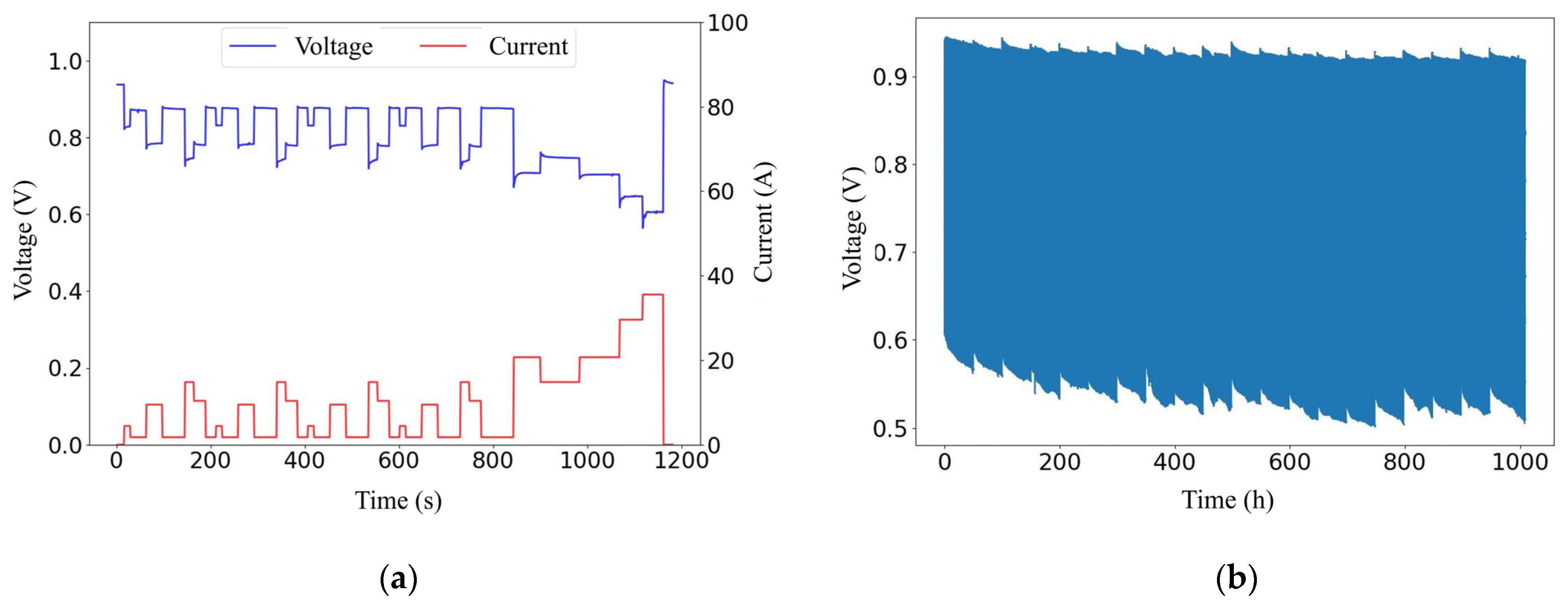
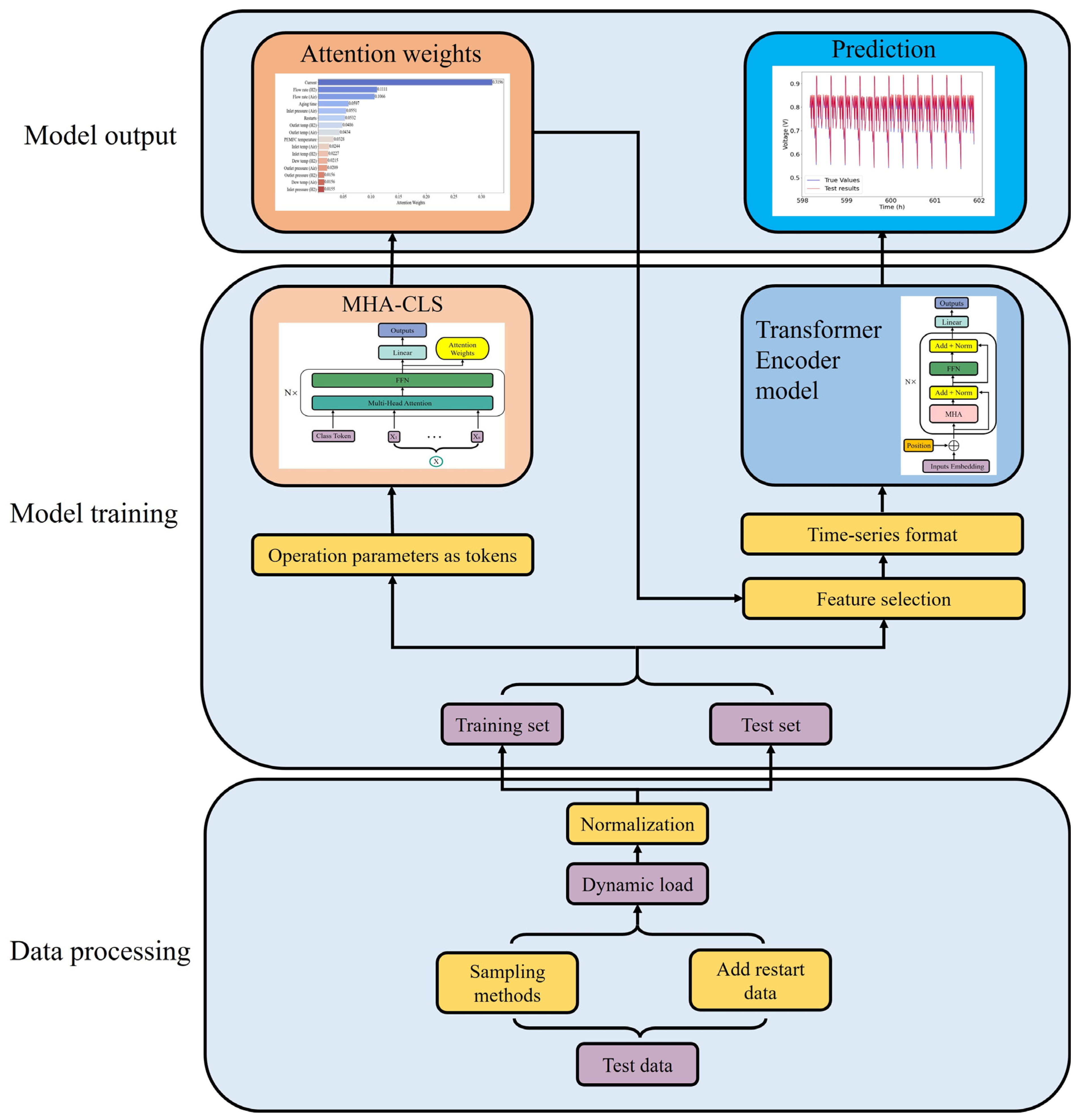
• Data processing: To analyze the performance of the PEMFC under dynamic load cycle operating conditions, the dynamic cycle dataset is employed in this study. The data preprocessing methods used in this study are detailed in Section 3.1. The dynamic cycle dataset then undergoes normalization processes to ensure consistency.
• Designing the structure of MHA-CLS and Transformer Encoder models: The basic architecture of both models is determined based on their respective purpose. For the MHA-CLS, the model is structured to treat each operational parameter as an individual token to identify the contribution of each parameter to the prediction. The Transformer Encoder model is designed to process the time-series data in a sequence, leveraging its ability to capture long-range dependencies and temporal patterns for degradation prediction.
• Models training; After preprocessing, the dynamic cycle dataset is divided into a training set and a testing set with a predefined ratio. The models are trained by feeding them the dynamic cycle dataset, and the training process involves the optimizer and the evaluation criteria. In addition, various hyperparameters are set to optimize model performance.
• Performance prediction: Upon training completion, the trained MHA-CLS model is used to analyze the impact of varying operational parameters on performance, while the Transformer Encoder model predicts the aging trends of the PEMFC over time using selected operating parameters.

4. Simulation Results and Discussion

The proposed MHA-CLS and Transformer Encoder models were validated on the dynamic cycle dataset for their prediction performance under dynamic cycles. Additionally, selected operating parameters in the dynamic cycle dataset were used to evaluate the predictive capability of the Transformer Encoder model. The selection of hyperparameters is also introduced.

4.1. Evaluation Methods of Prediction Performance

To validate the prediction performance, it is necessary to establish a standard for evaluating the model’s goodness of fit and calculating the prediction error of the proposed model. This study introduces four evaluation metrics: the coefficient of determination (R²), mean squared error (MSE), mean absolute error (MAE), and root mean squared error (RMSE). An R² value of 1 indicates that the model’s output perfectly fits the original data, while for the other metrics, lower values indicate higher prediction accuracy. The corresponding mathematical expressions are summarized as follows:

$${\mathrm{R}}^2=1-{\displaystyle \frac{\sum _{\mathrm{i}=1}^{\mathrm{n}}({\mathrm{y}}_{\mathrm{i}}-{\widehat{\mathrm{y}}}_{\mathrm{i}}{)}^2}{\sum _{\mathrm{i}=1}^{\mathrm{n}}({\mathrm{y}}_{\mathrm{i}}-\overline{\mathrm{y}}{)}^2}}$$

(11)

$$\mathrm{M}\mathrm{S}\mathrm{E}={\displaystyle \frac{1}{\mathrm{n}}}\sum _{\mathrm{i}=1}^{\mathrm{n}}({\mathrm{y}}_{\mathrm{i}}-{\widehat{\mathrm{y}}}_{\mathrm{i}}{)}^2$$

(12)

$$\mathrm{M}\mathrm{A}\mathrm{E}={\displaystyle \frac{1}{\mathrm{n}}}\sum _{\mathrm{i}=1}^{\mathrm{n}}|{\mathrm{y}}_{\mathrm{i}}-{\widehat{\mathrm{y}}}_{\mathrm{i}}|$$

(13)

$$\mathrm{R}\mathrm{M}\mathrm{S}\mathrm{E}=\sqrt{{\displaystyle \frac{1}{\mathrm{n}}}\sum _{\mathrm{i}=1}^{\mathrm{n}}({\mathrm{y}}_{\mathrm{i}}-{\widehat{\mathrm{y}}}_{\mathrm{i}}{)}^2}$$

(14)

where ${\mathrm{y}}_{\mathrm{i}}$ represents the actual values, ${\widehat{\mathrm{y}}}_{\mathrm{i}}$ is the predicted values, $\overline{\mathrm{y}}$ is the mean of the actual values, and n is the total number of data points.

4.2. Simulation Results for MHA-CLS

The input to the MHA-CLS model consists of 16-dimensional operational parameters extracted at each time step from the dynamic cycling dataset. These 16 parameters include aging time, current, inlet and outlet pressures of hydrogen and air, PEMFC operating temperature, dew point temperatures of hydrogen and air, inlet and outlet temperatures of hydrogen and air, total stack flow rates of hydrogen and air, and number of restarts. Each operational parameter is treated as an individual token, allowing the model to extract attention weights from the class token to analyze its impact on PEMFC performance. The model’s predicted output serves as a performance metric for PEMFC, providing a basis for evaluating the model’s effectiveness in capturing the influence of operational parameters.

The hyperparameters of the MHA-CLS model are carefully selected to optimize prediction accuracy while ensuring computational efficiency. Key hyperparameters include number of attention heads, hidden layer dimension, number of MHA layers, dropout rate, learning rate, batch size, and number of training epochs. The number of attention heads determines the number of parallel attention mechanisms used within the MHA module. The hidden layer dimension defines the number of neurons in each hidden layer, influencing the model’s ability to learn complex patterns. The dropout rate helps prevent overfitting by randomly deactivating a fraction of neurons during training. The learning rate controls the step size for updating model parameters during training, balancing convergence speed and stability. The batch size specifies the number of samples processed simultaneously during training, affecting both training efficiency and generalization. The number of training epochs determines how many times the model processes the entire training dataset. In this study, the model employs four attention heads, a hidden dimension of 32, and a three-layer MHA structure. The specific hyperparameter combination also includes a dropout rate of 0.1, a learning rate of 0.001, a batch size of 50, and 100 training epochs.

Based on the established model, this study computed the prediction results for the dynamic cycle dataset. Regarding data partitioning, data collected within the time range of (0, 600) hours was used for model training, whereas data from (600, 1008) hours was designated for testing. The model prediction results are shown in Figure 7. From Figure 7a, the output voltage of the PEMFC in the dynamic durability test can be observed, and the output voltage variations observed during the dynamic durability test exhibit an apparent periodic behavior. This phenomenon is mainly caused by the interruptions that occur during the dynamic load cycle test mentioned in Section 3.1. The MHA-CLS model successfully captures and reproduces this periodic pattern. Since the dynamic cycle dataset contains a large number of test points covering the entire test process, the detailed prediction performance may not be clearly visible. Therefore, a specific segment is magnified for a more detailed analysis. Figure 7b highlights the transition between the training and testing phases, providing a clearer comparison of the model’s predictive performance at different stages.

Furthermore, Figure 8 illustrates the variation in loss during the model training process. Initially, the loss decreases rapidly, indicating the model is learning and improving. As the training progresses, the curve flattens, signaling that the model is converging towards the optimal solution.

From the error analysis results presented in

Table 2. Evaluation criteria analysis for MHA-CLS model.

Metric	RMSE	MSE	MAE	${\mathbf{R}}^2$
Training Phase	0.01517550	0.00023029	0.00998576	0.99375892
Test Phase	0.01784608	0.00031848	0.01170215	0.99026889

, the RMSE of the model during the training phase is 0.01517550, increasing slightly to 0.01784608 in the testing phase. The loss in the test phase is marginally higher than in the training phase, suggesting that the MHA-CLS model effectively mitigates the risk of overfitting and generalizes well to unseen data, further confirming its stability and reliability.

Upon verifying the reliability of the model, the attention mechanism of the MHA-CLS model was employed to analyze the influence of each input variable on the final prediction outcome. Specifically, by utilizing the attention weights of the class token, the contributions of all input features to the model’s decision-making process were quantified. The attention weights of the class token for all input features are illustrated in Figure 9. The results indicate that current, total stack flow rates of hydrogen, and total stack flow of air exhibit the highest attention weights, suggesting that these features exert the most significant impact on PEMFC performance predictions in the dynamic cycle dataset. The current reflects the electrochemical reaction rate and is related to catalyst sintering and the loss of active sites. Meanwhile, variations in total stack flow rates may cause membrane dehydration and local hotspots. Membrane drying induces mechanical stress and micro-cracks in the proton exchange membrane, resulting in its gradual degradation over time. Notably, the attention weights corresponding to aging time and restart times are also relatively high, signifying that these features contain substantial information relevant to PEMFC voltage changes in the dynamic cycle dataset, particularly in representing aspects of the performance degradation. They reflect the cumulative operational stress experienced by the fuel cell, including chemical degradation and mechanical fatigue within the fuel cell components. While these features are not as dominant as current and total stack flow rates, they provide supplementary information that enhances prediction accuracy.

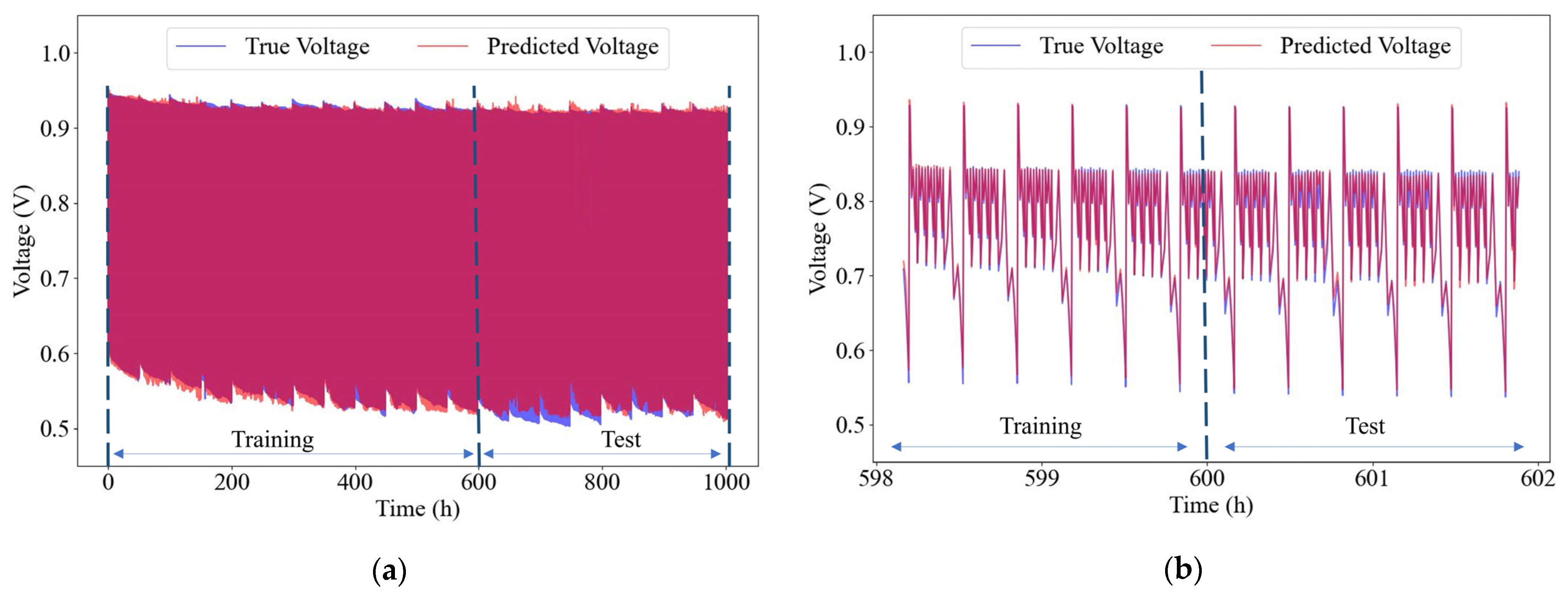
4.3. Prediction Results for Transformer Encoder Model

To validate the PEMFC degradation prediction capability of the Transformer Encoder model, tests were conducted using the dynamic dataset. In this setup, the Transformer Encoder model receives time-series tokens as the input, where each token consists of the operational parameters. In time-series modeling, a time window is often used to segment sequential data, allowing the model to capture temporal dependencies effectively.

In this study, data collected within the time range of (0, 600) hours is used for model training, while data from (600, 1008) hours is allocated for testing. Since the Transformer Encoder model requires time series data, its MHA layers need a more complex structure and more parameters. The Transformer Encoder model is designed with eight attention heads, a hidden dimension of 256, and a three-layer MHA structure. The selected hyperparameter combination includes a dropout rate of 0.1, a learning rate of 0.0001, a batch size of 100, and a total of 100 training epochs.

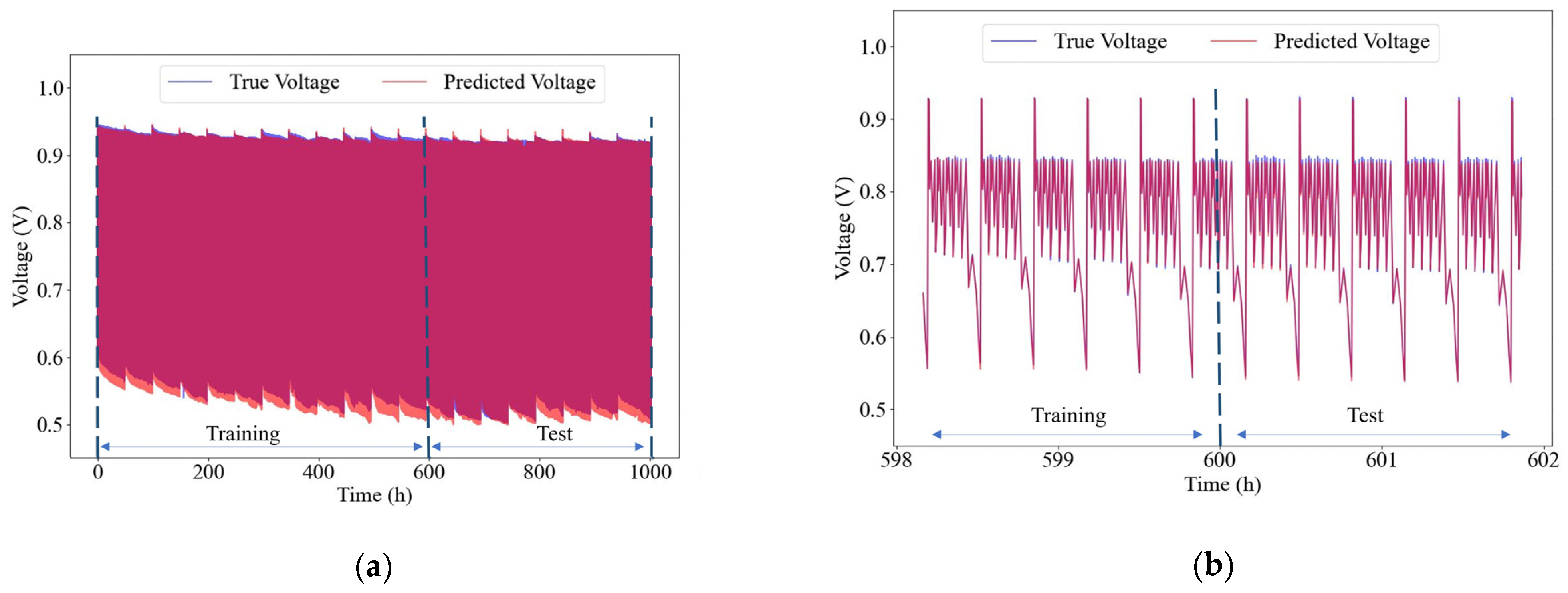
4.3.1. Prediction Performance with All Operational Parameters

The model prediction results are shown in Figure 10. As seen in Figure 10a, the Transformer Encoder model demonstrates strong prediction capability for the PEMFC output voltage in the dynamic durability test dataset. Figure 10b emphasizes the transition between the training and testing phases, offering a clearer comparison of the model’s performance across different stages. Figure 11 illustrates the loss change during the training process of the dynamic dataset, where the Transformer Encoder model exhibits a faster initial decline and reaches convergence towards the optimal solution more quickly compared to the MHA-CLS model.

In terms of the error analysis presented in

Table 3. Evaluation criteria analysis for Transformer Encoder model with all operational parameters.

Metric	RMSE	MSE	MAE	${\mathbf{R}}^2$
Training Phase	0.00497314	0.00002751	0.00387942	0.99925697
Test Phase	0.00895497	0.00008019	0.00659059	0.99035249

, during the training phase, the RMSE for the Transformer Encoder model with all operational parameters was 0.00497314, which increased slightly to 0.00895497 in the testing phase. The Transformer Encoder model showed excellent performance in predicting PEMFC performance degradation in terms of generalization and stability. The ability of the Transformer Encoder model to maintain a low error rate during both training and testing further emphasizes its robustness in real-world applications. In comparison, the MHA-CLS model showed higher RMSE values in both the training phase and test phase. The lower RMSE in the Transformer Encoder model can be attributed to the added complexity of incorporating time-series information and positional encoding. These additional features introduce more parameters into the model, which enhance the model’s representation.

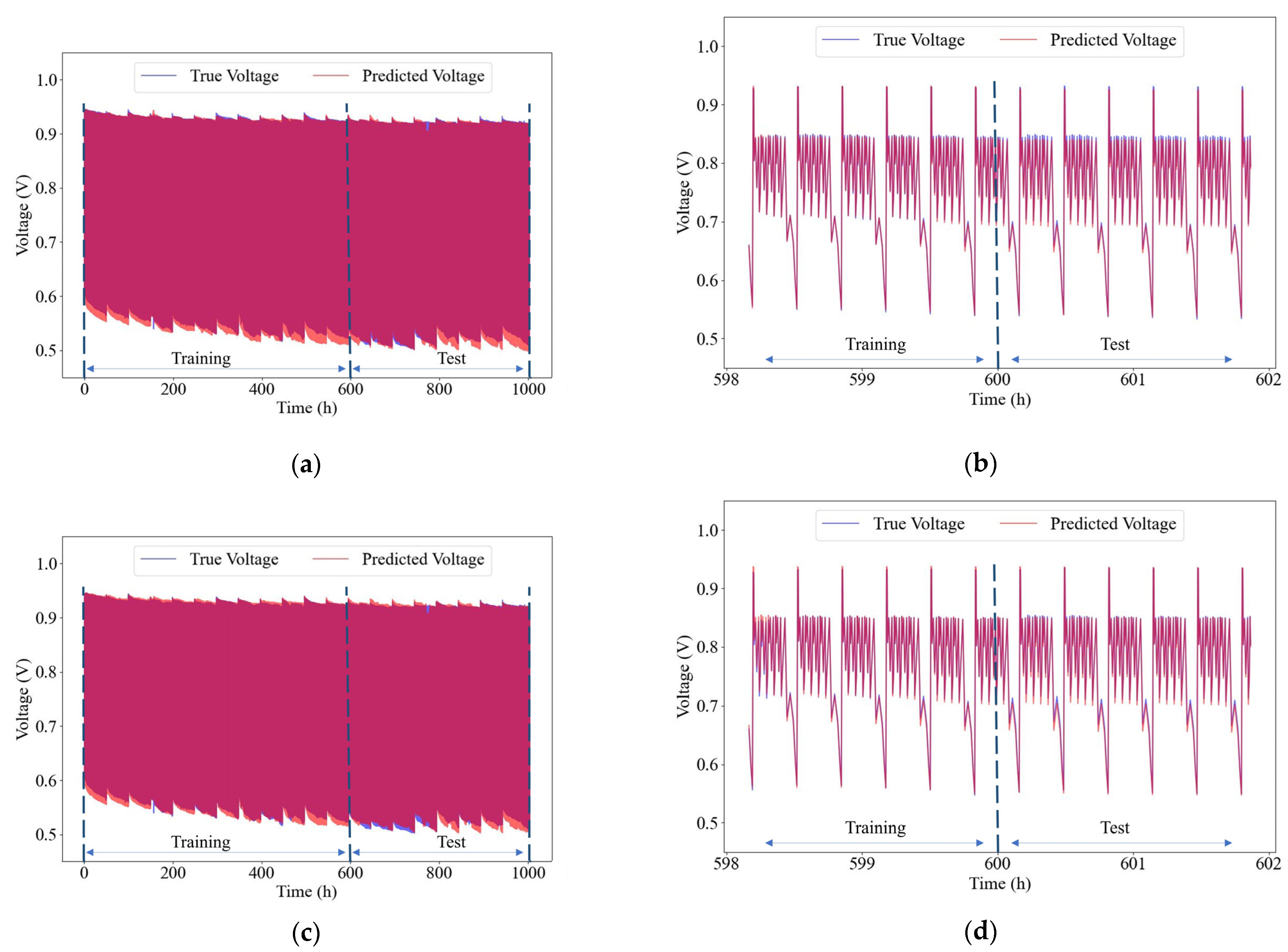
4.3.2. Prediction Performance with Selected Operational Parameters

The model validation continues with selected operational parameters. Based on the results in Section 4.2, different operational parameters have varying impacts on the prediction performance. Therefore, the top 11 and 8 most influential parameters were selected for separate evaluation according to Figure 9. These selections correspond to excluding features with the lowest 10% and 20% of the normalized attention weights derived from the MHA-CLS model results. These thresholds were chosen to systematically evaluate how different levels of feature reduction influence model performance while preserving the most informative inputs. The goal was to reduce the model complexity, lower the risk of overfitting, and thus improve the generalization ability of the model.

In Case 1, the eight most influential parameters were evaluated, corresponding to the eight-dimensional input. These parameters included current, total stack hydrogen flow, total stack air flow, aging time, air inlet pressure, number of restarts, hydrogen outlet temperature, and air outlet temperature. In Case 2, the 11 most influential parameters were evaluated, with the addition of the hydrogen and air inlet temperatures, as well as the PEMFC operating temperature. This case corresponded to the 11-dimensional input.

Figure 12 shows the prediction results. As seen in Figure 12a,c, the Transformer Encoder model still shows a strong prediction capability for the PEMFC output voltage with the selected operational parameters. Figure 12b,d provide a zoomed-in view of the transition between the training and testing phases, offering a more detailed comparison of the prediction results.

The evaluation criteria analysis for the Transformer Encoder model, as shown in

Table 4. Evaluation criteria analysis for Transformer Encoder model.

Metric	Training Phase			Test Phase
	16-Dim	8-Dim	11-Dim	16-Dim	8-Dim	11-Dim
RMSE	0.00497314	0.00578862	0.00466829	0.00895497	0.00924553	0.00878816
MSE	0.00002751	0.00003351	0.00002179	0.00008019	0.00009468	0.00007723
MAE	0.00387942	0.00441970	0.00345508	0.00659059	0.00717803	0.00645769
${\mathbf{R}}^2$	0.99925697	0.99911760	0.99944786	0.99035249	0.98701987	0.99070856

, compares the model’s performance across three different sets of operational parameters: 16-dimensional, 8-dimensional, and 11-dimensional. The results demonstrate that the 8-dimensional and 11-dimensional parameter sets retain most of the information present in the original 16-dimensional set, with only slight variations in performance. For both the training and test phases, the RMSE, MSE, MAE, and R² values for the 8-dimensional and 11-dimensional parameter sets are very close to those for the 16-dimensional set, suggesting that reducing the number of features does not significantly degrade the model’s predictive accuracy. In fact, the 11-dimensional set shows a marginal improvement in RMSE and ${\mathrm{R}}^2$ during the training phase, while the 8-dimensional set has similar or slightly higher error metrics, indicating that fewer features can still provide effective predictive performance. These results suggest that the selected operational parameters are roughly equivalent in information content to the original 16 parameters, demonstrating that the MHA-CLS feature selection reduces the input complexity of the Transformer Encoder model while preserving predictive performance and mitigating overfitting. This indicates that the combination of these approaches is meaningful.

4.3.3. Comparison with Other Works

This study compares the proposed approach with several existing works to provide a comprehensive comparison of the model performance.

Table 5. Comparison of predictions with RMSE in related literature.

Dataset	Method	Training Phase	Test Phase
Dynamic drive cycle dataset (0.6–0.95 V)	ANN [47]		0.0429
	SVM [47]		0.0294
	LSTM [30]	0.011066	0.017637
	GRU [30]	0.015873	0.018260
	LSTM attention [30]	0.008542	0.016409
	AT-MIXGU [33]	0.009975	0.011049
	Transformer Encoder(11-dim)	0.004668	0.008788
	Transformer Encoder(16-dim)	0.004973	0.008954
2500 h durability test dataset (210–365 V)	Informer [46]		0.75
	Improved Informer [46]		0.55

summarizes the reported RMSE values along with the corresponding experimental datasets. Ref. [46] used PEMFC degradation data from a 2500 h durability test of an onboard fuel cell system. Although the dataset in ref. [46] differs from the one used in this study, both involve complex voltage degradation behavior under dynamic load cycling, making the prediction task both relevant and valuable. As shown in Table 5, the Transformer Encoder model proposed in this study achieves higher prediction accuracy compared to the models used in the referenced works. Compared with LSTM attention and AT-MIXGU, which also use the attention mechanism, the RMSE of the Test Phase is reduced by 46.22% and 20.47%, respectively. This indicates that the proposed model is more effective in capturing the complex temporal patterns of PEMFC voltage degradation under dynamic operating conditions. The improved performance may be attributed to the model’s ability to extract and leverage long-range dependencies within the input sequence.

5. Conclusions

Facing the problem of voltage degradation in PEMFCs under dynamic operating conditions, this study proposes a neural network model based on MHA-CLS to analyze the influence of different input parameters. Subsequently, a Transformer Encoder model is developed to predict the long-term degradation trend of PEMFC voltage.

By analyzing the attention weight matrix generated by the MHA-CLS model, the contribution of each operational parameter to the output voltage prediction was quantified. This analysis revealed which parameters play a more significant role in the predication process, thereby providing insights into feature selection for model simplification and optimization.

The Transformer Encoder model achieved strong predictive performance under dynamic load cycle conditions, with an RMSE, MAE, and R² of 0.008954, 0.006590, and 0.990352 on the test phase, showing that the Transformer Encoder model is well-suited for the prediction of PEMFC performance degradation. Based on the feature importance analysis from the MHA-CLS model, a set of 11 key parameters was selected. When these selected inputs were used in the Transformer Encoder model, the prediction accuracy remained comparable to the full 16-parameter case. This confirms that the selected parameters retain most of the essential information, allowing the model to maintain high accuracy while helping mitigate overfitting and improving model generalizability.

For future work, the Transformer architecture can be further enhanced by integrating with other neural network modules. In addition, the framework could incorporate with decision-making modules to improve PEMFC lifespan and reliability through proactive management. Moreover, the use of datasets with longer testing durations is planned to further validate the model’s performance over extended operating periods.

References

1. Abe, J.O.; Popoola, A.; Ajenifuja, E.; Popoola, O.M. Hydrogen Energy, Economy and Storage: Review and Recommendation. Int. J. Hydrogen Energy 2019, 44, 15072–15086. [Google Scholar] [CrossRef]
2. Staffell, I.; Scamman, D.; Abad, A.V.; Balcombe, P.; Dodds, P.E.; Ekins, P.; Shah, N.; Ward, K.R. The Role of Hydrogen and Fuel Cells in the Global Energy System. Energy Environ. Sci. 2019, 12, 463–491. [Google Scholar] [CrossRef]
3. Khalili, S.; Rantanen, E.; Bogdanov, D.; Breyer, C. Global Transportation Demand Development with Impacts on the Energy Demand and Greenhouse Gas Emissions in a Climate-Constrained World. Energies 2019, 12, 3870. [Google Scholar] [CrossRef]
4. Cano, Z.P.; Banham, D.; Ye, S.; Hintennach, A.; Lu, J.; Fowler, M.; Chen, Z. Batteries and Fuel Cells for Emerging Electric Vehicle Markets. Nat. Energy 2018, 3, 279–289. [Google Scholar] [CrossRef]
5. Un-Noor, F.; Padmanaban, S.; Mihet-Popa, L.; Mollah, M.N.; Hossain, E. A Comprehensive Study of Key Electric Vehicle (EV) Components, Technologies, Challenges, Impacts, and Future Direction of Development. Energies 2017, 10, 1217. [Google Scholar] [CrossRef]
6. Aminudin, M.; Kamarudin, S.; Lim, B.; Majilan, E.; Masdar, M.; Shaari, N. An Overview: Current Progress on Hydrogen Fuel Cell Vehicles. Int. J. Hydrogen Energy 2023, 48, 4371–4388. [Google Scholar] [CrossRef]
7. Wu, J.; Yuan, X.Z.; Martin, J.J.; Wang, H.; Zhang, J.; Shen, J.; Wu, S.; Merida, W. A Review of PEM Fuel Cell Durability: Degradation Mechanisms and Mitigation Strategies. J. Power Sources 2008, 184, 104–119. [Google Scholar] [CrossRef]
8. Tanç, B.; Arat, H.T.; Baltacıoğlu, E.; Aydın, K. Overview of the next Quarter Century Vision of Hydrogen Fuel Cell Electric Vehicles. Int. J. Hydrogen Energy 2019, 44, 10120–10128. [Google Scholar] [CrossRef]
9. Raeesi, M.; Changizian, S.; Ahmadi, P.; Khoshnevisan, A. Performance Analysis of a Degraded PEM Fuel Cell Stack for Hydrogen Passenger Vehicles Based on Machine Learning Algorithms in Real Driving Conditions. Energy Convers. Manag. 2021, 248, 114793. [Google Scholar] [CrossRef]
10. Ahmadi, P.; Torabi, S.H.; Afsaneh, H.; Sadegheih, Y.; Ganjehsarabi, H.; Ashjaee, M. The Effects of Driving Patterns and PEM Fuel Cell Degradation on the Lifecycle Assessment of Hydrogen Fuel Cell Vehicles. Int. J. Hydrogen Energy 2020, 45, 3595–3608. [Google Scholar] [CrossRef]
11. Pei, P.; Chen, H. Main Factors Affecting the Lifetime of Proton Exchange Membrane Fuel Cells in Vehicle Applications: A Review. Appl. Energy 2014, 125, 60–75. [Google Scholar] [CrossRef]
12. Ren, P.; Pei, P.; Li, Y.; Wu, Z.; Chen, D.; Huang, S. Degradation Mechanisms of Proton Exchange Membrane Fuel Cell under Typical Automotive Operating Conditions. Prog. Energy Combust. Sci. 2020, 80, 100859. [Google Scholar] [CrossRef]
13. Nguyen, H.L.; Han, J.; Nguyen, X.L.; Yu, S.; Goo, Y.-M.; Le, D.D. Review of the Durability of Polymer Electrolyte Membrane Fuel Cell in Long-Term Operation: Main Influencing Parameters and Testing Protocols. Energies 2021, 14, 4048. [Google Scholar] [CrossRef]
14. Strahl, S.; Gasamans, N.; Llorca, J.; Husar, A. Experimental Analysis of a Degraded Open-Cathode PEM Fuel Cell Stack. Int. J. Hydrogen Energy 2014, 39, 5378–5387. [Google Scholar] [CrossRef]
15. Dhimish, M.; Vieira, R.G.; Badran, G. Investigating the Stability and Degradation of Hydrogen PEM Fuel Cell. Int. J. Hydrogen Energy 2021, 46, 37017–37028. [Google Scholar] [CrossRef]
16. Song, K.; Ding, Y.; Hu, X.; Xu, H.; Wang, Y.; Cao, J. Degradation Adaptive Energy Management Strategy Using Fuel Cell State-of-Health for Fuel Economy Improvement of Hybrid Electric Vehicle. Appl. Energy 2021, 285, 116413. [Google Scholar] [CrossRef]
17. Hahn, S.; Braun, J.; Kemmer, H.; Reuss, H.-C. Optimization of the Efficiency and Degradation Rate of an Automotive Fuel Cell System. Int. J. Hydrogen Energy 2021, 46, 29459–29477. [Google Scholar] [CrossRef]
18. Zuo, B.; Cheng, J.; Zhang, Z. Degradation Prediction Model for Proton Exchange Membrane Fuel Cells Based on Long Short-Term Memory Neural Network and Savitzky-Golay Filter. Int. J. Hydrogen Energy 2021, 46, 15928–15937. [Google Scholar] [CrossRef]
19. Chandesris, M.; Vincent, R.; Guetaz, L.; Roch, J.-S.; Thoby, D.; Quinaud, M. Membrane Degradation in PEM Fuel Cells: From Experimental Results to Semi-Empirical Degradation Laws. Int. J. Hydrogen Energy 2017, 42, 8139–8149. [Google Scholar] [CrossRef]
20. Mayur, M.; Strahl, S.; Husar, A.; Bessler, W.G. A Multi-Timescale Modeling Methodology for PEMFC Performance and Durability in a Virtual Fuel Cell Car. Int. J. Hydrogen Energy 2015, 40, 16466–16476. [Google Scholar] [CrossRef]
21. Pei, P.; Chang, Q.; Tang, T. A Quick Evaluating Method for Automotive Fuel Cell Lifetime. Int. J. Hydrogen Energy 2008, 33, 3829–3836. [Google Scholar] [CrossRef]
22. Ou, M.; Zhang, R.; Shao, Z.; Li, B.; Yang, D.; Ming, P.; Zhang, C. A Novel Approach Based on Semi-Empirical Model for Degradation Prediction of Fuel Cells. J. Power Sources 2021, 488, 229435. [Google Scholar] [CrossRef]
23. Vichard, L.; Harel, F.; Ravey, A.; Venet, P.; Hissel, D. Degradation Prediction of PEM Fuel Cell Based on Artificial Intelligence. Int. J. Hydrogen Energy 2020, 45, 14953–14963. [Google Scholar] [CrossRef]
24. Napoli, G.; Ferraro, M.; Sergi, F.; Brunaccini, G.; Antonucci, V. Data Driven Models for a PEM Fuel Cell Stack Performance Prediction. Int. J. Hydrogen Energy 2013, 38, 11628–11638. [Google Scholar] [CrossRef]
25. Huo, W.; Li, W.; Zhang, Z.; Sun, C.; Zhou, F.; Gong, G. Performance Prediction of Proton-Exchange Membrane Fuel Cell Based on Convolutional Neural Network and Random Forest Feature Selection. Energy Convers. Manag. 2021, 243, 114367. [Google Scholar] [CrossRef]
26. Ming, W.; Sun, P.; Zhang, Z.; Qiu, W.; Du, J.; Li, X.; Zhang, Y.; Zhang, G.; Liu, K.; Wang, Y.; et al. A Systematic Review of Machine Learning Methods Applied to Fuel Cells in Performance Evaluation, Durability Prediction, and Application Monitoring. Int. J. Hydrogen Energy 2023, 48, 5197–5228. [Google Scholar] [CrossRef]
27. Chen, K.; Badji, A.; Laghrouche, S.; Djerdir, A. Polymer Electrolyte Membrane Fuel Cells Degradation Prediction Using Multi-Kernel Relevance Vector Regression and Whale Optimization Algorithm. Appl. Energy 2022, 318, 119099. [Google Scholar] [CrossRef]
28. Wilberforce, T.; Biswas, M. A Study into Proton Exchange Membrane Fuel Cell Power and Voltage Prediction Using Artificial Neural Network. Energy Rep. 2022, 8, 12843–12852. [Google Scholar] [CrossRef]
29. Sahajpal, K.; Rana, K.P.S.; Kumar, V. Accurate Long-Term Prognostics of Proton Exchange Membrane Fuel Cells Using Recurrent and Convolutional Neural Networks. Int. J. Hydrogen Energy 2023, 48, 30532–30555. [Google Scholar] [CrossRef]
30. Zuo, J.; Lv, H.; Zhou, D.; Xue, Q.; Jin, L.; Zhou, W.; Yang, D.; Zhang, C. Deep Learning Based Prognostic Framework towards Proton Exchange Membrane Fuel Cell for Automotive Application. Appl. Energy 2021, 281, 115937. [Google Scholar] [CrossRef]
31. Yu, Y.; Yu, Q.; Luo, R.; Chen, S.; Yang, J.; Yan, F. A Predictive Framework for PEMFC Dynamic Load Performance Degradation Based on Feature Parameter Analysis. Int. J. Hydrogen Energy 2024, 71, 1090–1103. [Google Scholar] [CrossRef]
32. Li, S.; Luan, W.; Wang, C.; Chen, Y.; Zhuang, Z. Degradation Prediction of Proton Exchange Membrane Fuel Cell Based on Bi-LSTM-GRU and ESN Fusion Prognostic Framework. Int. J. Hydrogen Energy 2022, 47, 33466–33478. [Google Scholar] [CrossRef]
33. Yang, Y.; Yang, Y.; Zhou, S.; Li, H.; Zhu, W.; Liu, Y.; Xie, C.; Zhang, R. Degradation Prediction of Proton Exchange Membrane Fuel Cell Based on Mixed Gated Units under Multiple Operating Conditions. Int. J. Hydrogen Energy 2024, 67, 268–281. [Google Scholar] [CrossRef]
34. Ramesh, A.S.; Vigneshwar, S.; Vickram, S.; Manikandan, S.; Subbaiya, R.; Karmegam, N.; Kim, W. Artificial Intelligence Driven Hydrogen and Battery Technologies–A Review. Fuel 2023, 337, 126862. [Google Scholar] [CrossRef]
35. Pan, R.; Yang, D.; Wang, Y.; Chen, Z. Performance Degradation Prediction of Proton Exchange Membrane Fuel Cell Using a Hybrid Prognostic Approach. Int. J. Hydrogen Energy 2020, 45, 30994–31008. [Google Scholar] [CrossRef]
36. Lv, L.; Pei, P.; Ren, P.; Wang, H.; Wang, G. Exploring Performance Degradation of Proton Exchange Membrane Fuel Cells Based on Diffusion Transformer Model. Energies 2025, 18, 1191. [Google Scholar] [CrossRef]
37. Bahdanau, D.; Cho, K.; Bengio, Y. Neural Machine Translation by Jointly Learning to Align and Translate. In Proceedings of the International Conference on Learning Representations, Banff, AB, Canada, 14–16 April 2014. [Google Scholar]
38. Vaswani, A.; Shazeer, N.; Parmar, N.; Uszkoreit, J.; Jones, L.; Gomez, A.N.; Kaiser, Ł.; Polosukhin, I. Attention Is All You Need. In Advances in Neural Information Processing Systems; MIT Press: Cambridge, MA, USA, 2017; Volume 30. [Google Scholar]
39. Dosovitskiy, A.; Beyer, L.; Kolesnikov, A.; Weissenborn, D.; Zhai, X.; Unterthiner, T.; Dehghani, M.; Minderer, M.; Heigold, G.; Gelly, S.; et al. An Image Is Worth 16x16 Words: Transformers for Image Recognition at Scale. arXiv 2020, arXiv:2010.11929. [Google Scholar]
40. Devlin, J.; Chang, M.-W.; Lee, K.; Toutanova, K. Bert: Pre-Training of Deep Bidirectional Transformers for Language Understanding. In Proceedings of the 2019 Conference of the North American Chapter of the Association for Computational Linguistics: Human Language Technologies, Volume 1 (Long and Short Papers), Minneapolis, MN, USA, 2–7 June 2019; pp. 4171–4186. [Google Scholar]
41. Lu, J.; Batra, D.; Parikh, D.; Lee, S. Vilbert: Pretraining Task-Agnostic Visiolinguistic Representations for Vision-and-Language Tasks. In Advances in Neural Information Processing Systems; MIT Press: Cambridge, MA, USA, 2019; Volume 32. [Google Scholar]
42. Zamir, S.W.; Arora, A.; Khan, S.; Hayat, M.; Khan, F.S.; Yang, M.-H. Restormer: Efficient Transformer for High-Resolution Image Restoration. In Proceedings of the IEEE/CVF Conference on Computer Vision and Pattern Recognition, New Orleans, LA, USA, 18–24 June 2022; pp. 5728–5739. [Google Scholar]
43. Zerveas, G.; Jayaraman, S.; Patel, D.; Bhamidipaty, A.; Eickhoff, C. A Transformer-Based Framework for Multivariate Time Series Representation Learning. In Proceedings of the 27th ACM SIGKDD Conference on Knowledge Discovery & Data Mining, Online, 14–18 August 2021; pp. 2114–2124. [Google Scholar]
44. Touvron, H.; Cord, M.; Douze, M.; Massa, F.; Sablayrolles, A.; Jégou, H. Training Data-Efficient Image Transformers & Distillation through Attention. In Proceedings of the International Conference on Machine Learning, PMLR, Online, 18–24 July 2021; pp. 10347–10357. [Google Scholar]
45. Zuo, J.; Lv, H.; Zhou, D.; Xue, Q.; Jin, L.; Zhou, W.; Yang, D.; Zhang, C. Long-Term Dynamic Durability Test Datasets for Single Proton Exchange Membrane Fuel Cell. Data Brief 2021, 35, 106775. [Google Scholar] [CrossRef]
46. Tang, X.; Shi, L.; Li, M.; Xu, S.; Sun, C. Health State Estimation and Long-Term Durability Prediction for Vehicular PEM Fuel Cell Stacks Under Dynamic Operational Conditions. IEEE Trans. Power Electron. 2025, 40, 4498–4509. [Google Scholar] [CrossRef]
47. Nagulapati, V.M.; Kumar, S.S.; Annadurai, V.; Lim, H. Machine Learning Based Fault Detection and State of Health Estimation of Proton Exchange Membrane Fuel Cells. Energy AI 2023, 12, 100237. [Google Scholar] [CrossRef]
Figure 1. Structures of attention mechanism.
Energies 18 03177 g001
Figure 2. Structures of multi-head attention.
Energies 18 03177 g002
Figure 3. Multi-Head Attention with Class Token Model.
Energies 18 03177 g003
Figure 4. The Transformer Encoder model architecture.
Energies 18 03177 g004
Figure 5. Diagram of the: (a) single FC-DLC cycle and (b) the durability test.
Energies 18 03177 g005
Figure 6. The workflow schematic diagram.
Energies 18 03177 g006
Figure 7. Simulation results for MHA-CLS: (a) training and prediction results; (b) part of the results.
Energies 18 03177 g007
Figure 8. Training loss for MHA-CLS.
Energies 18 03177 g008
Figure 9. The attention weights of the class token for all input features.
Energies 18 03177 g009
Figure 10. Simulation results for Transformer Encoder model with all operational parameters: (a) training and prediction results; (b) part of the results.
Energies 18 03177 g010
Figure 11. Training loss for Transformer Encoder model with all operational parameters.
Energies 18 03177 g011
Figure 12. Simulation results for the Transformer Encoder model with selected operational parameters. (a) Training and prediction results with 8 parameters; (b) part of the results with 8 parameters; (c) training and prediction results with 11 parameters; (d) part of the results with 11 parameters.
Energies 18 03177 g012