A Multi-Scale Time–Frequency Complementary Load Forecasting Method for Integrated Energy Systems

Abstract

With the growing demand for global energy transition, integrated energy systems (IESs) have emerged as a key pathway for sustainable development due to their deep coupling of multi-energy flows. Accurate load forecasting is crucial for IES optimization and scheduling, yet conventional methods struggle with complex spatio-temporal correlations and long-term dependencies. This study proposes ST-ScaleFusion, a multi-scale time–frequency complementary hybrid model to enhance comprehensive energy load forecasting accuracy. The model features three core modules: a multi-scale decomposition hybrid module for fine-grained extraction of multi-time-scale features via hierarchical down-sampling and seasonal-trend decoupling; a frequency domain interpolation forecasting (FI) module using complex linear projection for amplitude-phase joint modeling to capture long-term patterns and suppress noise; and an FI sub-module extending series length via frequency domain interpolation to adapt to non-stationary loads. Experiments on 2021–2023 multi-energy load and meteorological data from the Arizona State University Tempe campus show that ST-ScaleFusion achieves 24 h forecasting MAE values of 667.67 kW for electric load, 1073.93 kW/h for cooling load, and 85.73 kW for heating load, outperforming models like TimesNet and TSMixer. Robust in long-step (96 h) forecasting, it reduces MAE by 30% compared to conventional methods, offering an efficient tool for real-time IES scheduling and risk decision-making.

1. Introduction

Under dual requirements of accelerated global industrialization and high-quality economic and social development, the contradiction between the sharp decline in fossil energy reserves and the sharp increase in environmental carrying pressure has become increasingly prominent [1,2]. This prompts the energy system to urgently undergo structural transformations so as to achieve sustainable development goals. The conventional energy system is limited by the inherent mode of single-energy flow independent planning and operation, which makes it difficult for different energy forms to form effective complementarity [3], further leading to problems such as low energy conversion efficiency and insufficient waste heat recovery [4,5]. In this context, the integrated energy system has achieved deep coupling and joint optimization of multiple energy flows such as electric, heating, and cooling by constructing a “source–grid–load” collaborative regulation mechanism, and fully unleashes the synergistic effects of multi-energy complementarity [6,7]. In addition, a 2012 study of the State Grid Corporation of China revealed that for every 1% increase in load forecasting accuracy, a power loss of approximately 58 GWh is expected to be reduced per year [8]. This number continues to increase with the increase in total electricity consumption, highlighting the fundamental role of high-accuracy load forecasting in planning, design, optimization, and scheduling of the IES.

To solve the many problems caused by inaccurate load forecasting, many scholars have conducted research on the accuracy of such forecasting problems. The development of load forecasting methods can be roughly divided into two stages. In the first stage, conventional statistical methods, such as the linear regression [9,10], the exponential smoothing method [11], and the moving average method [12] are mostly used. Although the statistical methods can effectively utilize historical data, they are difficult to use to capture complex nonlinear correlations, have poor model performance when facing big data problems, and rely heavily on past patterns, resulting in limited forecasting performance. Therefore, with the rapid development of artificial intelligence, machine learning methods such as Support Vector Machine (SVM), Decision Tree (DT), and Random Forest (RF) have become more effective in handling load forecasting problems. In this case, the second stage of load forecasting has begun, and a large quantity of artificial intelligence methods represented by machine learning have emerged.

In recent years, deep learning technology has achieved good results in many fields with its powerful feature extraction ability [13,14,15,16]. In the field of single-load forecasting, Wang et al. proposed a hybrid model combining Long Short-Term Memory and Transformer [17]. Temporal dependency of power load is captured by using LSTM, and feature extraction at key time points is enhanced by using an attention mechanism of Transformer. This significantly improves the accuracy of short-term power load forecasting. Li et al. developed, through research, an integrated model of adaptive wavelet decomposition and a Convolutional Gated Recurrent Unit [18]. In this method, multi-scale features of load signals are extracted through adaptive wavelet decomposition, and high-dimensional feature fusion is implemented by using the CNN-GRU to effectively solve the forecasting problem of non-stationary load signals. Huang et al. applied a spatio-temporal graph convolutional network (ST-GCN) for region-level load forecasting [19]. By constructing a spatial topology diagram between power nodes and integrating time series features, this method implements modeling of complex spatial correlations in a distributed power grid. Zhang et al. proposed a probabilistic load forecasting method based on deep reinforcement learning [20]. In this method, the forecasting interval is dynamically optimized by using the Actor–Critic framework, which overcomes the limitations of conventional quantile regression in uncertain modeling and provides more reliable interval forecasting for risk decision-making in the electricity market. In the field of multi-load forecasting, taking into consideration the coupling relationship between multiple energy loads, Chen et al. proposed a multi-load forecasting framework that combines variational mode decomposition and multi-task learning [21]. By decomposing the electric, heating, and cooling load signals into multi-modal components through VMD, and designing a joint optimization and forecasting objective between a task-sharing layer and a task-specific layer, the problem of multi-energy flow coupling feature extraction has been solved. Wu et al. constructed a multi-energy load forecasting model based on a graph attention network [22]. In this method, the dynamic coupling relationship between electric, heating, and gas loads are modeled over GAT, and LSTM is introduced to capture time dependency. This results in the error being reduced by 22% in multi-energy collaborative scenarios in industrial parks. Wang et al. proposed a deep Bayesian neural network with embedded physical constraints [23]. By incorporating the energy conservation equation as a regularization term into the loss function, this method satisfies both high accuracy and physical consistency requirements in multivariate load forecasting. In this way, the method is particularly applicable to high=proportion renewable energy scenarios. Zhuang et al. proposed a multi-scale spatio-temporal graph convolutional network in which the time-varying coupling features of multiple energy loads are captured through a multi-scale graph neural network [24]. By using the gated temporal convolution module, this method implements synchronous forecasting of multi-time-scale loads in the urban integrated energy system, with a 30% increase in calculation efficiency in comparison with the conventional methods.

In recent years, various uncertainty analysis methods have been applied to integrated energy load forecasting models in order to provide decision-makers with more comprehensive and reliable information. Yan et al. proposed a hybrid probability forecasting model based on CEEMDAN-LSTM-GPQR that quantifies the uncertainty by using a prediction interval [25]. This method significantly improves the accuracy of predictions. Furthermore, the composite evaluation factor has also been validated as effective. Li et al. introduced an innovative composite evaluation factor (CEF) that reconstructs the modal components after considering that their complexity, coupling, and frequency significantly reduced error accumulation [26]. In terms of reducing computation time, Zhang et al. utilized the Optimal Condition Decomposition (OCD) technique to break down the complex temporal model into a set of time-discrete parallel subproblems, significantly enhancing computational efficiency [27]. Zhang et al. proposed a multi-time-scale safety assessment and rolling adjustment strategy based on the Global Sensitivity Factor (GSF) for the asynchronous dynamic characteristics of electric–thermal systems [28]. This study addressed the resolution limitations of traditional discretization models in capturing thermal dynamic processes by constructing a continuous temperature mapping function and quantified the coupling relationships within the system through sensitivity analysis, providing a cross-scale collaborative control framework for the safe operation of integrated energy systems.

Existing machine learning methods have achieved great success in the field of comprehensive energy load forecasting. However, with the advancement of time series forecasting technologies, the methods for comprehensive energy forecasting have become more diverse and efficient. This study proposes a model ST-ScaleFusion for comprehensive energy forecasting. The main contributions are listed as follows:

This study utilizes a multi-layer down-sampling module to process the original time series while preserving the original time series of various scales, so that series features of various scales are obtained and more details about information about past time series are obtained.

Feature decomposition on time series of various scales is performed in the frequency domain by using the PFM module, different feature integration methods are selected based on the features of each sub-series, and an integrated series is then fused in the time domain, so that the effect of capturing time–frequency features simultaneously is achieved.

This study uses the FI module to extend the length of the input series through frequency domain interpolation, which effectively models long-term patterns and enhances the ability of the model to capture long-range dependency. In addition, by leveraging the strong adaptability of the frequency domain interpolation mechanism to non-stationary time series, the generalization ability of the model is effectively improved. In this way, more accurate load forecasting is eventually implemented.

The main contributions of this article can be attributed to the following points:

(I)

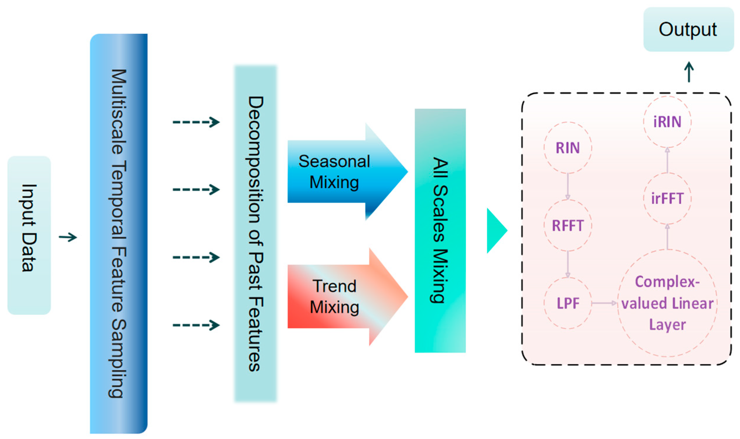
This study proposes the ST-ScaleFusion model, which achieves time–frequency complementary modeling through multi-scale temporal decomposition and frequency domain interpolation, thereby enabling the integrated modeling of temporal dynamics and frequency domain characteristics.

(II)

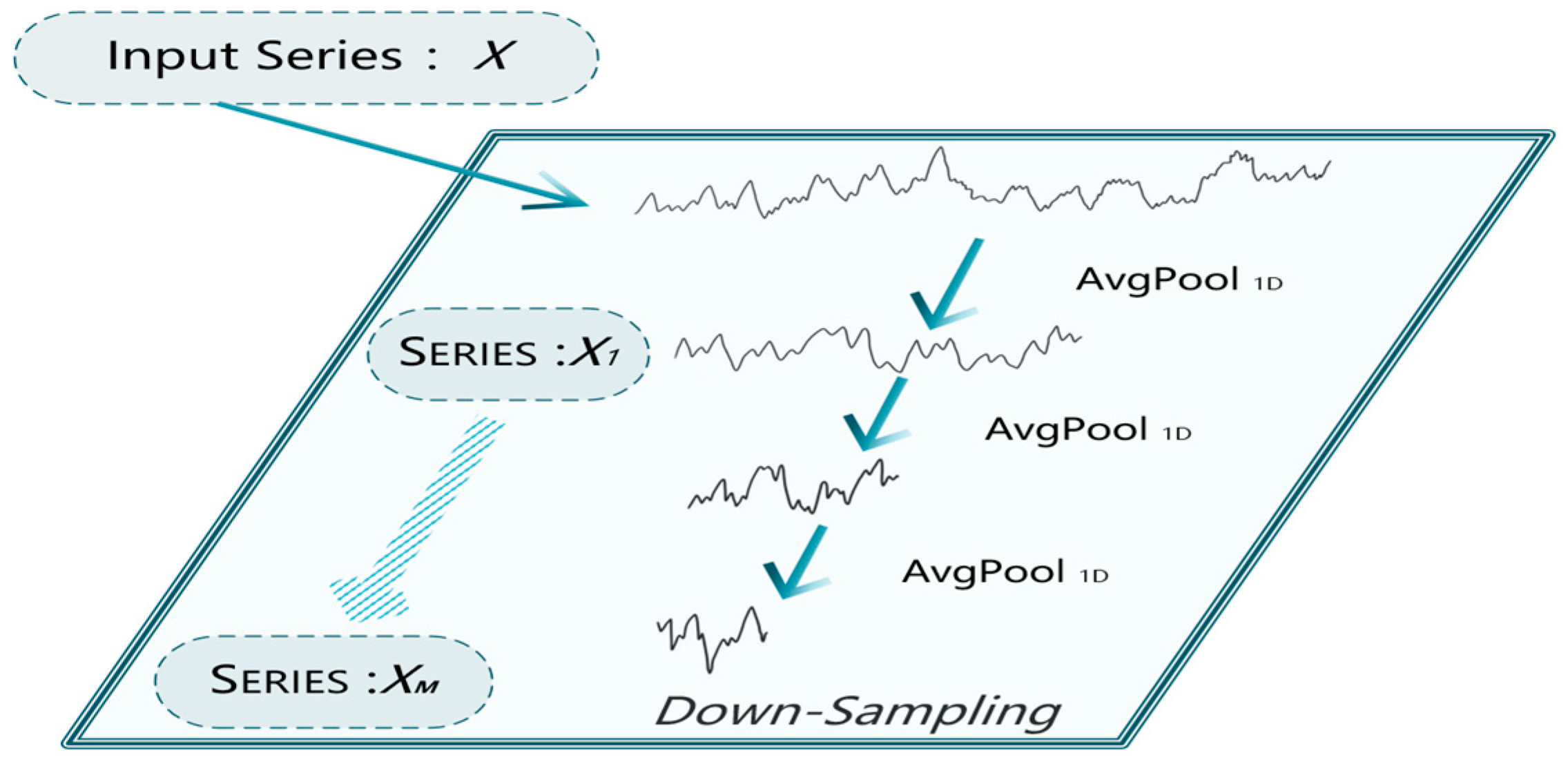
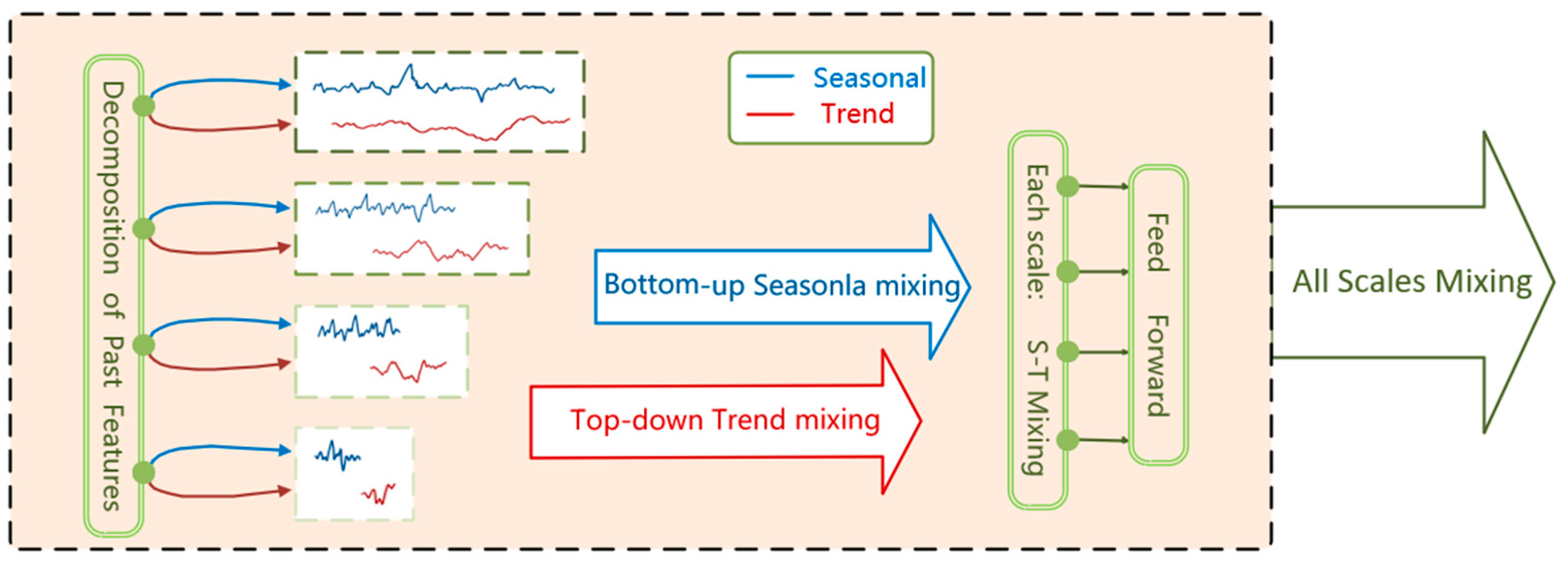
This study designs a hierarchical down-sampling and season-trend decoupling module to enhance multi-time-scale feature extraction capabilities, separating seasonal patterns from trend components to improve the interpretability and accuracy of long-term dependencies.

(III)

This study constructs a frequency domain interpolation module, realizing long-sequence modeling and noise suppression through complex linear projection in the frequency domain, which mitigates information loss in long-range forecasting and enhances anti-noise robustness.

(IV)

This study demonstrates significant superiority over traditional methods in multi-step forecasting tasks, providing an efficient tool for real-time scheduling in Intelligent Energy Systems by balancing prediction accuracy and computational efficiency.

2. Feature Analysis and Methods

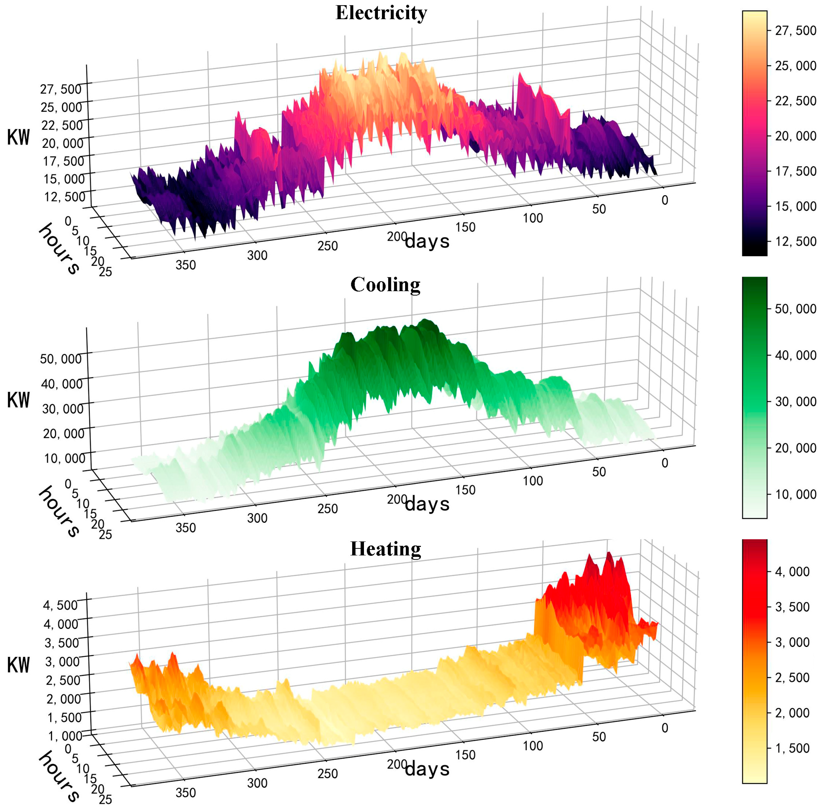
2.1. Data Analysis

2.1.1. Data Preprocessing

Given that the energy data approximately conforms to a normal distribution, and the time complexity of the standard deviation method (denoted as $\mathsf{O}(\mathrm{n}$)) is substantially lower than that of the boxplot method (denoted as $\mathsf{O}\left(\mathrm{n}\mathrm{l}\mathrm{o}\mathrm{g}\right(\mathrm{n}\left)\right)$), this approach more effectively satisfies the stringent low-latency requirements inherent in energy scheduling tasks. Consequently, in the data preprocessing phase of this study, the standard deviation method is adopted. This choice is underpinned by the method’s computational efficiency, which aligns with the operational demands of real-time energy management systems, thereby ensuring optimal performance in handling large-scale energy datasets while meeting latency constraints.

Although some methods perform better in certain scenarios, there are the following limitations in this study. For instance, Kalman filtering requires the establishment of a state-space model in advance, while the nonlinear characteristics of energy loads and certain meteorological factors are difficult to model accurately. In contrast, ordinary linear interpolation can effectively preserve the trend characteristics of the load while offering advantages in computational efficiency, which is why it has become the primary choice for this study.

In this study, outlier detection was first conducted using the standard deviation method. After the data outliers are removed, missing values are processed according to the value interpolation method in Formula (1) to ensure data integrity. To ensure consistent dimensionality of the input data, this study normalizes the data according to Formula (2), where x_i′ is a normalized value, x_i is the ith input value, min(x) corresponds to a minimum value in a dataset, and max(x) indicates a maximum value in the dataset.

$$x_i={\displaystyle \frac{1}{4}}(x_{i-2}+x_{i-1}+x_{i+1}+x_{i+2})$$

(1)

$$x_i^{\prime }={\displaystyle \frac{x_i-\min (x)}{\max (x)-\min (x)}}+1$$

(2)

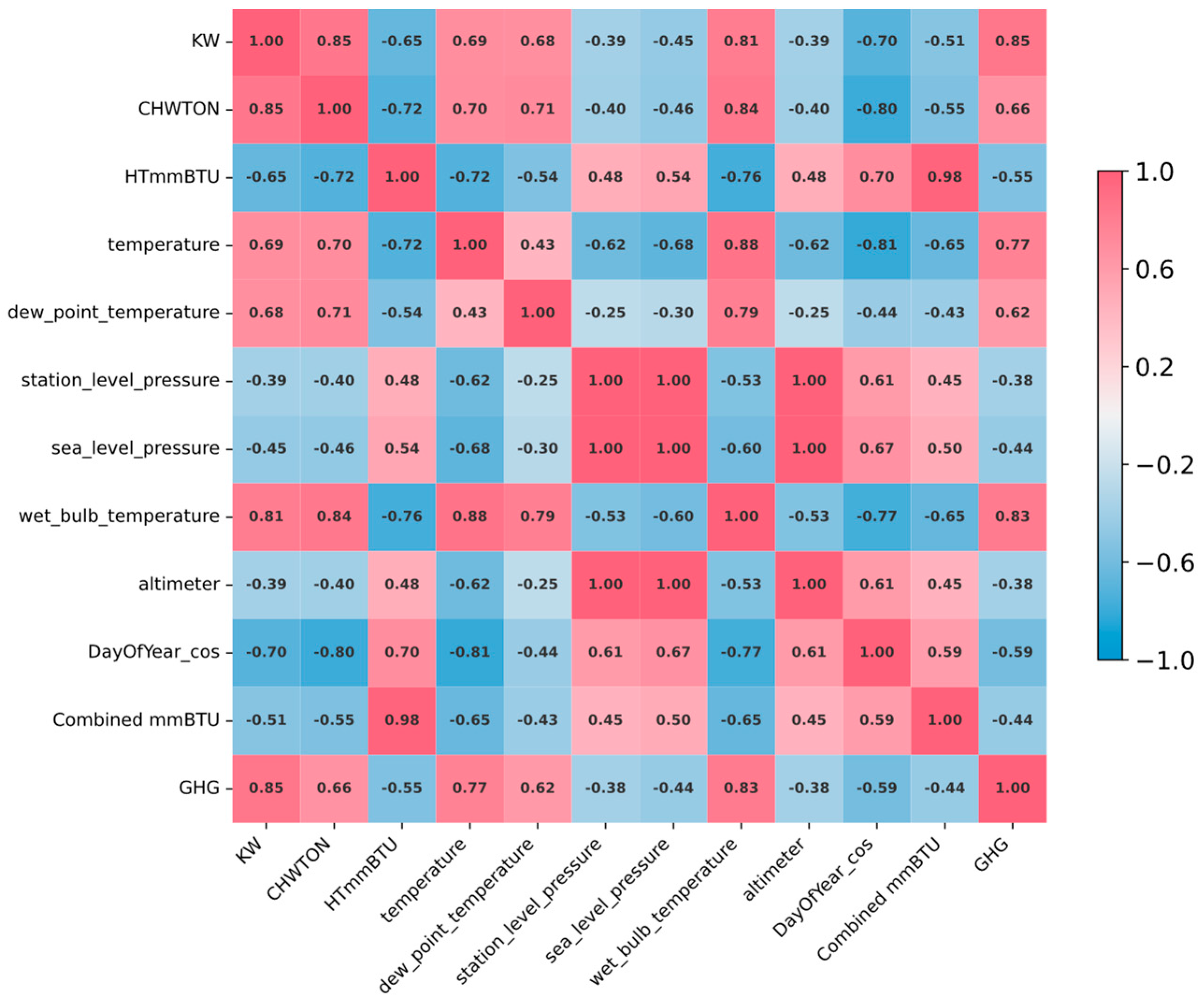
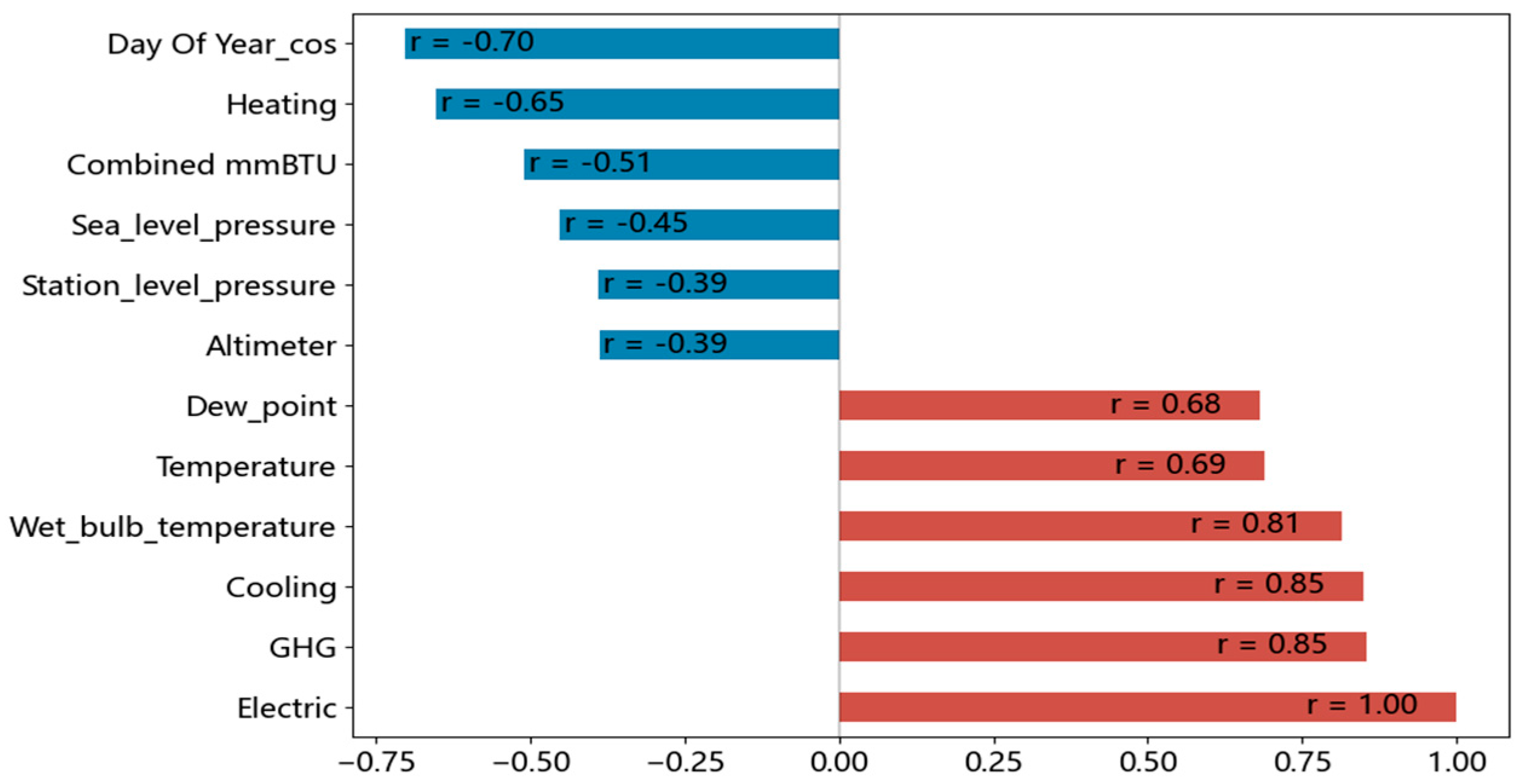
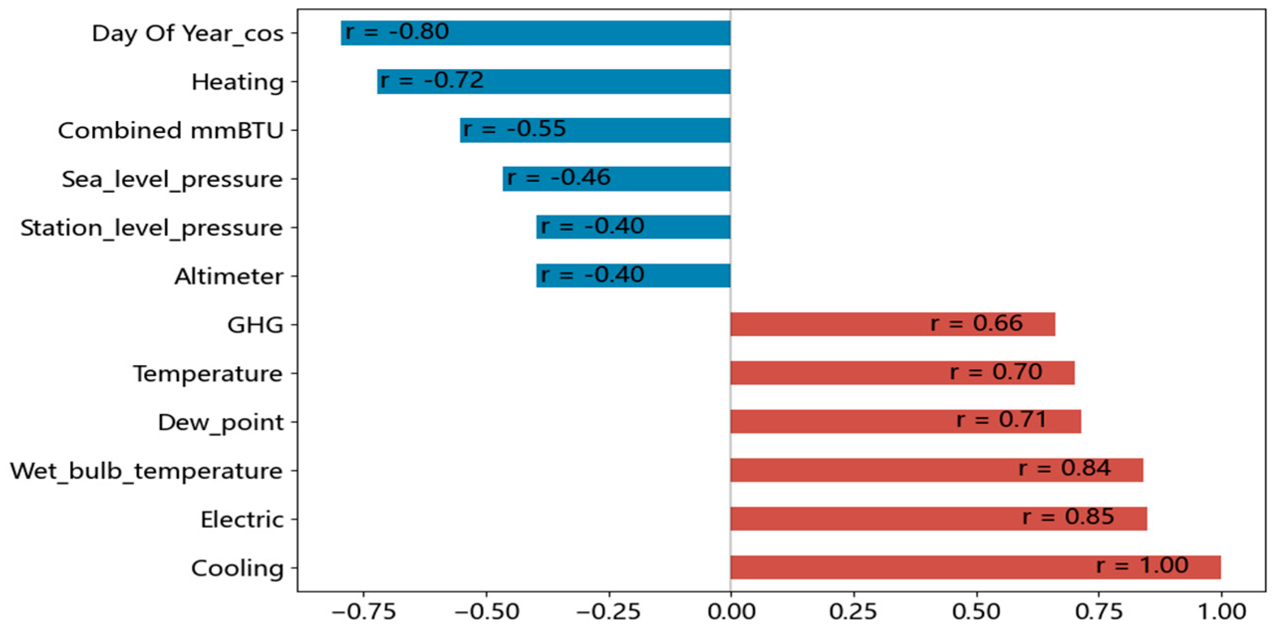
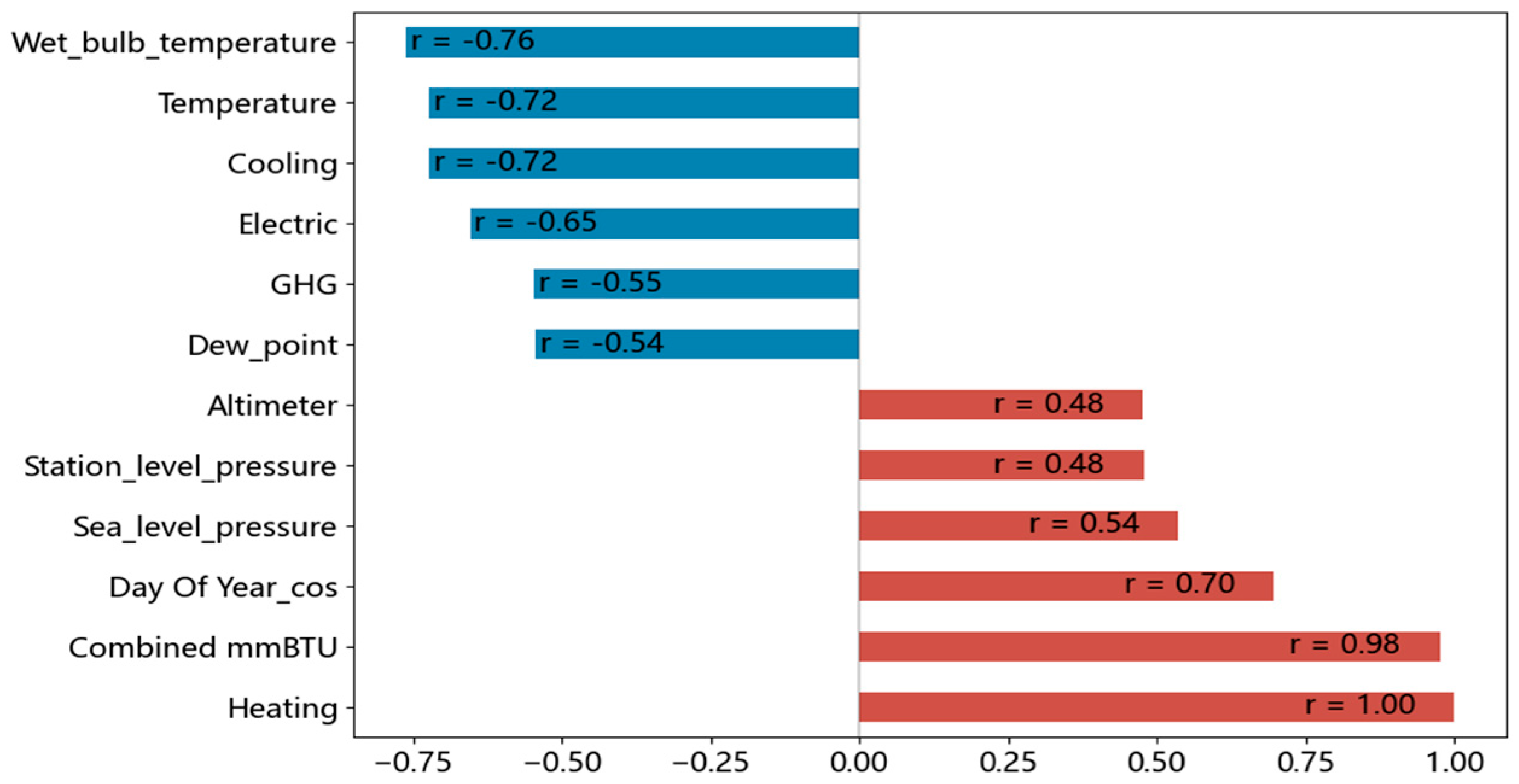
2.1.2. Data Correlation Analysis

In addition to the inherent feature of the load, external factors also have a significant impact on changes in the load. This study incorporates electric, temperature, wet bulb temperature, dew point, altimeter, and sea-level pressure as input variables. In addition, station-level pressure is also taken into consideration to assess its impact on load changes. To visually illustrate correlations between multiple energy loads and meteorological factors, the Pearson coefficient is used to analyze linear correlations between the variables in this study. The Pearson correlation coefficient, as a measure of linear correlation, is used to accurately visualize the strength of the linear relationship between two variables.

Statistically speaking, an absolute value of this coefficient is positively correlated with the strength of linear correlation between variables. Specifically, when the Pearson correlation coefficient ranges from 0.8 to 1.0, it is usually considered that there is a highly significant linear positive correlation between two variables, meaning that changes in one variable will highly consistently trigger changes in the other variable in the same direction and almost proportionally. Alternatively, when the value ranges from 0.6 to 0.8, it indicates a strong linear correlation between variables. Although the degree of collaborative change is slightly lower than the previous situation, it still shows a relatively obvious linear trend. Alternatively, when the coefficient is in the range of 0.4 to 0.6, it indicates a moderate linear correlation between variables and changes in variables begin to show a specific degree of correlation, but the regularity is weakened in comparison with that of the strong correlation. Alternatively, in the range of 0.2 to 0.4, there is only a weak linear correlation between variables, and the impact of changes of one variable on another is relatively limited. Alternatively, when the correlation coefficient is in the range of 0.0 to 0.2, it strongly implies that the linear correlation between variables is extremely weak, which can be almost ignored in actual application scenarios. In other words, it is considered that there is no obvious linear dependency relationship between the two. The calculation results of this study are shown in the following Figure 1.

Correlations between electric, cooling, and heating loads and other meteorological factors are separately visualized. It can be seen that the absolute values of correlation coefficients between electric, cooling, and heating loads are all greater than 0.6, indicating a strong linear correlation between multiple energy loads. In addition, absolute correlation coefficients between the meteorological factors and the multiple energy loads in the dataset are all greater than or equal to 0.4, indicating that there is also an undeniable relationship between the multiple energy loads and the meteorological factors. To clearly understand the correlation degrees between different energy loads and various features, we analyze the correlation values of the “electric”, “cooling”, and “heating” loads with other features. Figure 2 illustrates the correlation coefficients of the “electric” load with each feature, showing its positive and negative correlations.

Figure 3 presents a similar analysis for the “cooling” load, revealing its association patterns with different features. Figure 4 focuses on the “heating” load, displaying its correlation values with each feature to further aid in understanding the influencing factors of the heating load.

2.2. Methods

The principal objective of this research is to utilize the past observed values of electric load, cooling load, heating load, and diverse meteorological factors to derive the most probable future forecasted values for the electric load, cooling load, and heating load. Essentially, this constitutes a time series forecasting task, where the crux of accurate forecasting resides in the comprehensive extraction of hidden information from historical time series and the minimization of the influence of interfering factors to the greatest extent possible. Consequently, this research proposes a multi-scale time–frequency complementary hybrid forecasting model. The core forecasting architecture of this research comprises a cascaded multi-scale decomposition hybrid module and a frequency domain interpolation forecasting module. The framework of our model can be seen in Figure 5.

2.2.1. Multi-Scale Decomposition Module

For the complex spatio-temporal coupling features of multiple energy loads in the integrated energy system, the multi-scale decomposition hybrid module with a hierarchical feature extraction capability is first constructed. A schematic of the module is shown in Figure 6.

A historical observed series $X=[x_1,\dots ,x_P{]}^T\in {\mathbb{R}}^{P\times d}$ ($d$ is a dimension of meteorological variables and multi-energy load variables) whose length is $P$ is provided, and a multi-scale series set $\{X_m{\}}_{m=0}^M$ is generated through average pooling, where $X_m\in {\mathbb{R}}^{\lfloor P/2^m\rfloor \times d}$ indicates the $m$th level of down-sampling series. This process can be formalized as:

$$X_m={\mathrm{AvgPool}}_{1D}\left(X_{m-1}\right),m=1,\dots M,$$

(3)

2.2.2. Past Feature Mixing Module

When conducting in-depth research on past observed data, this study finds that due to the complexity of real-world time series, even series of a scale at a coarsest granularity often exhibit hybrid changes. To effectively decouple seasonal fluctuations and trend evolution in load series, this study uses stacked multi-scale fusion modules to mix past information of different scales. The module adopts a dual-path hybrid mechanism. The data processing procedure of the module is shown in Figure 7. In this module, seasonal time series are indicated in red, and trend time series are indicated in blue, to provide clearer descriptions of the data-processing procedure of the series.

Considering the significant differences in the features of seasonal and trend components, this study performs seasonal trend decomposition on the series of each scale. In the formula below, we use SD to denote the seasonal trend decomposition algorithm and MA to represent the moving average algorithm [29].

$$\begin{array}{cc}\hfill { S}_m^{\left(l\right)},T_m^{\left(l\right)}& =\mathrm{S}\mathrm{D}\left(X_m^{\left(l\right)}\right)\hfill \\ \hfill S_m^{\left(l\right)}& =X_m^{\left(l\right)}-\mathrm{M}\mathrm{A}(X_m^{\left(l\right)},k)\hfill \\ \hfill T_m^{\left(l\right)}& =\mathrm{M}\mathrm{A}\left(X_m^{\left(l\right)},k\right),\hfill \end{array}$$

(4)

where $\mathrm{MA}(\cdot )$ indicates the sliding average operator, $k$ indicates the window size, and $l$ indicates the stacked multi-scale fusion module layer index.

In the seasonal analysis, long periodicities can be referred to as an aggregation of short periodicities. This indicates the importance of detailed information in forecasting future seasonal changes, as information of time series of a lower level and a fine scale can be integrated upwards to supplement detailed information for coarser-scale seasonal modeling. Therefore, when conducting seasonal mixing, a bottom-up hybrid strategy is adopted for seasonal components, and cross-scale information transfer is implemented through learnable linear projection ${ \mathcal{W}}_s^{m\to m+1}$:

$$S_{m+1}^{\left(l\right)}\leftarrow S_{m+1}^{\left(l\right)}+\sigma \left({\mathcal{W}}_s^{m\to m+1}{S}_m^{\left(l\right)}\right)$$

(5)

In the trend analysis, this study finds that detailed changes in trend terms may introduce noise, while time series of coarse scales are more likely to provide macro information. Therefore, a top-down hybrid method is adopted, and high-level coarse-scale knowledge is used to guide low-level fine-scale trend modeling. Trend components are mixed, and a macro trend is transferred by using a weight matrix ${\mathcal{W}}_t^{m+1\to m}$:

$$T_m^{\left(l\right)}\leftarrow T_m^{\left(l\right)}+\sigma \left({\mathcal{W}}_t^{m+1\to m}{T}_{m+1}^{\left(l\right)}\right)$$

(6)

Cross-channel interaction is implemented through a multi-layer perceptron:

$$X_{ST}^{\left(l\right)}=A(S_m^{\left(l\right)}\oplus T_m^{\left(l\right)})+B$$

(7)

Finally, residual connections are included to enhance the attention of important features while implementing high-level to low-level trend information exchange:

$$X_m^{(l+1)}=X_m^{\left(l\right)}+X_{ST}^{\left(l\right)}$$

(8)

Multi-scale fusion is set to capture details of short-term load fluctuations (for example, daily electricity consumption periodicities) of a fine scale and extract long-term evolution patterns (for example, a seasonal heating demand) of a coarse scale. At the same time, optimization of decoupling of seasonal trend components of various scales is maintained. Through multi-scale complementary forecasting, the modeling ability of complex energy coupling relationships is significantly improved.

2.2.3. Frequency Domain Interpolation Forecasting Module (FI Module)

To overcome the problem of insufficient modeling of long-term dependency in a conventional time domain forecasting model, this study innovatively introduces frequency domain dynamic system modeling. Provided that longer time series have higher frequency resolution in their frequency indication, this study implements interpolation training and fitting on the frequency indication of the input time series segments, so as to extend the time series segments. Specifically, the study uses a single complex-value linear layer to learn the interpolation process, and to learn the amplitude scaling and phase shift operations corresponding to complex multiplication in interpolation operations. Generally, this module first uses the real fast Fourier transform to map time series segments to the complex frequency domain, completes interpolation operations, and then maps the frequency indication back to the time domain through inverse real fast Fourier transform.

• Frequency Domain Feature Modeling

Before introducing the specific methodologies, we will first discuss the rationality of addressing temporal issues in the frequency domain. According to Parseval’s theorem in Fourier analysis, the energy of a time domain signal is strictly conserved with its frequency domain representation. The formula is as follows:

$${\sum }_{\mathrm{t}=1}^{\mathrm{N}}{\left|\mathrm{x}\right(\mathrm{t}\left)\right|}^2={\displaystyle \frac{1}{\mathrm{N}}}{\sum }_{f=1}^{\mathrm{N}/2}{\left|\mathrm{X}\right(f\left)\right|}^2$$

(9)

where $\mathrm{x}\left(\mathrm{t}\right)$ denotes the time domain signal and $\mathrm{X}\left(f\right)$ represents the complex-value frequency domain representation. This property ensures the physical significance of frequency domain interpolation operations—by adjusting the amplitude and phase of frequency domain components, a reasonable extension of the time domain signal can be achieved under the premise of energy conservation.

The temporal translation of a signal is directly analogous to a phase shift in the frequency domain. Specifically, within the complex frequency domain, such phase shifts can be mathematically characterized through the multiplication of a complex exponential factor unit with the corresponding phase term. Formally, a signal $\mathrm{x}\left(\mathrm{t}\right)$ subjected to a time shift of $\mathsf{\tau }$ units forward is considered, yielding the shifted signal $\mathrm{x}(\mathrm{t}-\mathsf{\tau })$. The Fourier transform of this time-shifted signal is given by:

$${\mathrm{X}}_{\mathsf{\tau }}\left(f\right)=e^{-j2\pi f\mathsf{\tau }}\mathrm{X}\left(f\right)=\left|\mathrm{X}\right(f\left)\right|e^{-j\left(\theta \right(f)-2\pi f\mathsf{\tau })}=\left[\cos \left(2\pi f\mathsf{\tau }\right)-\mathrm{j}\sin \left(2\pi f\mathsf{\tau }\right)\right]\mathrm{X}\left(f\right)$$

(10)

This formulation underscores the linear relationship between time displacement and phase modulation in the frequency domain.

A detailed discussion on the processing of data in this module is presented here. Firstly, reversible instance-wise normalization (Reversible Instance-wise Normalization) is performed on the features that are denoted as $Z\in {\mathbb{R}}^{L\times d_{model}}$ and that are output by the multi-scale fusion module. This operation adjusts a signal to a distribution with zero mean and unit variance by independently calculating the mean and standard deviation for each channel to effectively eliminate direct current components (zero frequency component). The specific formula is:

$$\mathrm{Z}={\displaystyle \frac{z-\mu }{\sigma }},\mathsf{\mu }={\displaystyle \frac{1}{\mathrm{L}}}{\sum }_{\mathrm{i}=1}^{\mathrm{L}}{\mathrm{z}}_{\mathrm{i}},\sigma =\sqrt{{\displaystyle \frac{1}{\mathrm{L}}}{{\sum }_{\mathrm{i}=1}^{\mathrm{L}}({\mathrm{z}}_{\mathrm{i}}-\mathsf{\mu })}^2}$$

(11)

A normalized signal retains the fluctuation features of the original data. At the same time, the effectiveness of frequency domain indication is improved. A normalized output feature $Z\in {\mathbb{R}}^{L\times d_{model}}$ is mapped to the frequency domain through real-value fast Fourier transform:

$$\mathcal{F}\left(Z\right)=\mathrm{r}\mathrm{F}\mathrm{F}\mathrm{T}\left(Z\right)=[A,\mathsf{\Phi }]$$

(12)

Low-frequency components below the cut-off frequency are retained. Through this operation, calculation redundancy is reduced. In addition, the ability of the model to capture key frequency patterns by filtering out noise is improved.

• Frequency Domain Interpolation Module

Complex multiplication naturally supports simultaneous adjustment of an amplitude and a phase. This avoids information fragmentation caused by separate processing of the amplitude and the phase in a conventional real number network. Therefore, to establish a temporal dynamic extrapolation mechanism, complex-value linear projection is designed to implement frequency domain interpolation in this study. The frequency domain interpolation module is configured to control the model output length, and its core is to introduce an interpolation rate ${ \alpha }_{freq}$. It represents the ratio of the model’s output length $L_{out}$ to its corresponding input length $L_{in}$. Frequency interpolation is performed on a normalized complex frequency representation that is half the length of the original time series. It can be learned from the formula below that the interpolation rate in the frequency domain is equal to the interpolation rate α.

$${\alpha }_{freq}={\displaystyle \frac{L_{out}/2}{L_{in}/2}}={\displaystyle \frac{L_{out}}{L_{in}}}=\alpha$$

(13)

This indicates that the interpolation rate α can be directly applied to the frequency domain to implement unified control of the output length. An interpolated frequency domain signal is extended to a target length through zero padding. In a multivariate task, all channels share a same set of complex weights, and the detailed calculation process is as follows:

$$\begin{array}{rr}{\hat{A}}_f& ={\mathcal{W}}_a{\tilde{A}}_t\hfill \\ {\stackrel{\mathrm{ˆ}}{\mathsf{\Phi }}}_f& ={\mathcal{W}}_{\varphi }{\tilde{\mathsf{\Phi }}}_t+\Delta \varphi \hfill \end{array}$$

(14)

where ${\mathcal{W}}_a\in {\mathbb{C}}^{F\times L}$, ${\mathcal{W}}_{\varphi }\in {\mathbb{C}}^{F\times L}$ indicate an interpolation weight matrix, and $\Delta \varphi$ explicitly models a phase offset.

• Time Domain Mapping Module

This module converts a forecasting result back to the time domain through inverse Fourier transform and maps a forecasted series to a scale of the original input series through inverse normalization. The inverse Fourier transform process is as follows:

$$\hat{Y}=\mathrm{i}\mathrm{r}\mathrm{F}\mathrm{F}\mathrm{T}(\hat{A}\odot e^{j\stackrel{\mathrm{ˆ}}{\mathsf{\Phi }}})$$

(15)

This operation synthesizes a time domain signal by accumulating sine waves of frequency components, and a high-frequency component with zero padding corresponds to a smooth extension of the time domain. Then, inverse normalization uses the mean and standard deviation stored in the normalization stage to restore the original range of the data.

For multi-energy load forecasting, the frequency domain indication can effectively ensure information integrity by using the Parseval theorem, the intensity evolution and periodic shift in the load can be separately captured through amplitude-phase separation modeling, and the robustness to noise interference can be effectively improved through low-pass filtering. Finally, extracted features are projected onto the forecasting space. A main part of the entire process can be described as:

$$\begin{array}{c}\begin{array}{cc}\hfill \left\{X_m\right\}& ={\mathsf{\Gamma }}_{\mathrm{ms}}\left(X\right)\hfill \\ \hfill Z& ={\displaystyle \underset{m=0}{\overset{M}{⨁}}}{\mathsf{\Psi }}_{\mathrm{mixing}}\left(X_m\right)\hfill \\ \hfill \hat{Y}& ={\mathsf{{\rm Y}}}_{\mathrm{freq}}\left(Z\right)\hfill \end{array}\end{array}$$

(16)

where $\mathsf{\Gamma }$ indicates multi-scale decomposition, $\mathsf{\Psi }$ is a mixing operator, and $\mathsf{{\rm Y}}$ indicates frequency domain forecasting. This cascaded structure implements progressive optimization from time domain feature decoupling to frequency domain dynamic modeling, where the hierarchical features extracted by the multi-scale module provide a strong indication basis for frequency domain interpolation, and the frequency domain module transforms the forecasting problem into a differentiable spectral space interpolation task by using a physically inspired amplitude-phase dynamic system to effectively improve the accuracy of forecasting multiple energy load variables.

3. Results of Experiment

This article uses data from the metabolism project at the Arizona State University Tempe campus as the dataset of the experiment. The campus metabolism program has comprehensively collected all energy consumption data of the university, including for electric load, cooling load, and heating load. The standard unit for electric load is kilowatts (kW), the unit for cooling load is tons per hour, and the unit for heating load is British thermal units per hour (BTUs/h). For unified measurement, basic units of data related to electric, cooling, and heating loads are converted to kilowatts. Meteorological data can be downloaded from the official website of the National Renewable Energy Laboratory (NREL) in the United States. In this case, it is necessary to choose the weather station nearest to the Tampa campus. In this study, a total of 1042 days of hourly multi-energy load data and meteorological data are selected from 2021 to 2023. The forecasting step size is set to one hour.

In terms of experiment setup, the hardware platform is equipped with Intel Core i7-13700 KF CPU and Nvidia GeForce RTX 4070Tisuper GPU. In terms of software, the Python 3.13.1 programming language combined with the PyTorch 2.3.0 framework is used. The scale of the model is calculated as follows:

Total Parameters: 499,546

Model Size: 0.47640419006347656 megabytes (MB)

Computational Flops: 35.95 MMac

Training Time for 50 Epochs: 283.21 s

In addition, the experiment encompasses twelve features sampled at 23,807 time points (hourly intervals). For all forecasting horizon experiments, the dataset is partitioned into training, validation, and test sets at an 8:1:1 ratio.

3.1. Experimental Data Processing

Unpredictable disasters such as power outages, gas supply interruptions, measurement equipment failures, noise interference, and data transmission errors may result in abnormal and missing values during the data collection process, thereby reducing the forecasting accuracy of the forecasting model. To resolve this issue, the box plot quartile detection algorithm and the first-order exponential smoothing algorithm are used to identify outliers in time series. Any such outlier is to be marked as NaN (Not a Number) and is then filled by using a linear interpolation method to ensure data quality and relative integrity. After performing outlier detection and handling missing values, a total of 23,807 records are retained, as shown in Figure 8.

3.2. Comparative Experiment

This study conducts a preliminary analysis by taking 168 h of results from a specific week in the forecasting outputs. From the fitting result, it can be learned that the model used in this study basically completes the basic fitting of the true-value curve, and in comparison with other models in the figure, it better grasps the trend of load changes and implements higher accuracy in forecasting. The following Figure 9 shows the electrical load forecasting results from the model used in this study and some widely used load forecasting models from this dataset. As shown in Figure 10, the forecasted curves of each model fit the real curve well. In contrast, the model in this study (orange) follows the changes of the truth value well at both peak and valley values, and the forecasted curve has a higher overlap with the truth value (blue). In the compared models, some models have lag or amplitude deviation during peak stages, indicating lower forecasting accuracy than the model in this study.

It can be observed from Figure 11 that this model also provides the most accurate prediction of heating load. In comparison with the compared models, the model of this study closely follows the truth value in most fluctuation intervals, especially when dealing with high-frequency small fluctuations, which shows its stability. Based on the foregoing three graphs, it can be learned that the model in this study has a better fit between the forecasted curve and the truth value in different load scenarios than the compared models (TimesNet, TSMixer, and PatchTST), especially in capturing load fluctuation trends, peaks and valleys, and amplitudes. This indicates that the model has higher accuracy and stability in load forecasting tasks.

3.3. Comparison of Error Metrics

The following

Table 1. Comparison of multi-energy load forecasting results.

Models		Total Load				Electrical Load				Cooling Load				Heating Load
	Horizon	MAE	MAPE	RMSE	ACCR	MAE	MAPE	RMSE	ACCR	MAE	MAPE	RMSE	ACCR	MAE	MAPE	RMSE	ACCR
PatchTST	24	684.7	6.16	1153.5	0.946	816.5	5.46	1238.2	0.912	1146.3	8.08	1567.2	0.981	91.3	4.94	120.8	0.944
	48	903.8	8.08	1529.4	0.912	1044.5	6.85	1556.4	0.861	1548.4	10.91	2113.8	0.966	118.7	6.47	157.8	0.909
	72	1044.8	9.11	1756.7	0.887	1167.9	7.67	1735.3	0.826	1835.2	12.52	2474.4	0.954	131.3	7.14	175.0	0.881
	96	1196.4	10.43	1998.1	0.871	1290.3	8.35	1840.0	0.803	2159.2	15.32	2898.8	0.940	139.8	7.62	184.7	0.870
FiLM	24	709.5	6.36	1185.3	0.941	944.6	6.40	1377.9	0.890	1097.1	7.85	1521.9	0.981	87.0	4.83	119.0	0.950
	48	878.4	7.60	1489.7	0.916	1052.2	6.98	1554.8	0.857	1474.6	10.32	2027.0	0.967	108.3	5.50	143.6	0.924
	72	1030.7	9.06	1728.8	0.896	1180.3	7.79	1719.4	0.824	1789.0	12.89	2409.0	0.957	122.7	6.52	162.7	0.908
	96	1145.4	10.21	1887.9	0.880	1273.7	8.41	1817.3	0.803	2027.8	14.45	2676.0	0.946	134.8	7.78	177.5	0.891
NLinear	24	672.1	6.07	1134.4	0.946	856.9	5.81	1267.8	0.908	1072.6	7.57	1484.9	0.983	86.7	4.82	116.7	0.948
	48	881.9	7.70	1508.9	0.917	1060.5	7.10	1569.9	0.856	1479.9	10.37	2062.2	0.969	105.3	5.64	142.8	0.925
	72	1037.2	9.08	1742.8	0.895	1192.7	7.89	1731.1	0.823	1799.3	12.68	2432.6	0.956	119.7	6.66	159.7	0.906
	96	1155.3	9.99	1908.6	0.879	1286.2	8.60	1836.1	0.801	2048.1	14.39	2721.1	0.947	131.4	6.99	175.3	0.890
TimesNet	24	770.9	6.94	1244.4	0.933	1024.5	6.88	1443.6	0.881	1188.8	7.97	1594.8	0.983	99.3	5.98	126.5	0.935
	48	960.0	8.30	1598.7	0.906	1178.6	7.96	1652.7	0.838	1587.0	10.45	2176.2	0.968	114.2	6.48	147.8	0.914
	72	1064.0	8.94	1742.7	0.896	1278.7	8.60	1728.7	0.819	1794.7	11.56	2423.2	0.956	118.5	6.65	149.8	0.913
	96	1312.2	10.58	2173.3	0.859	1449.9	9.47	1978.8	0.764	2348.4	14.57	3060.7	0.933	138.3	7.69	174.9	0.880
TimeXer	24	700.1	6.25	1197.5	0.947	795.5	5.56	1218.3	0.916	1218.3	8.35	1672.9	0.979	86.5	4.82	118.4	0.946
	48	924.0	7.99	1591.8	0.916	984.4	6.78	1498.5	0.870	1679.5	11.42	2319.2	0.959	108.0	5.78	144.3	0.920
	72	1052.8	9.06	1795.2	0.895	1115.4	7.44	1698.8	0.835	1923.4	13.28	2649.3	0.947	119.6	6.46	158.4	0.904
	96	1172.5	10.07	1978.2	0.875	1196.3	7.79	1787.4	0.806	2188.7	15.37	2934.6	0.935	132.3	7.06	172.7	0.885
TSMixer	24	702.7	6.38	1185.7	0.942	897.1	5.99	1329.5	0.901	1123.4	8.32	1563.4	0.983	87.6	4.83	116.7	0.942
	48	919.5	7.80	1524.0	0.914	1063.0	7.00	1594.0	0.852	1587.4	10.53	2056.7	0.969	108.2	5.88	142.8	0.921
	72	1049.0	8.54	1744.3	0.898	1198.8	7.89	1781.1	0.821	1835.5	11.59	2448.1	0.960	112.8	6.13	148.6	0.913
	96	1184.4	9.76	1917.2	0.880	1298.2	8.69	1892.4	0.793	2132.7	13.84	2774.5	0.948	122.3	6.75	159.8	0.898
iTransformer	24	696.4	6.15	1159.4	0.946	831.8	5.48	1246.5	0.915	1165.6	7.99	1567.7	0.982	91.8	4.98	124.4	0.941
	48	948.0	8.09	1604.3	0.911	1066.2	6.97	1589.4	0.854	1667.8	11.35	2278.9	0.962	110.0	5.94	148.4	0.917
	72	1105.3	9.55	1833.1	0.889	1201.2	7.78	1745.4	0.823	1989.4	13.98	2666.1	0.950	125.1	6.90	169.8	0.895
	96	1187.2	10.27	1962.1	0.874	1260.8	8.15	1812.5	0.805	2167.4	15.25	2869.1	0.940	133.5	7.42	178.8	0.877
Crossformer	24	699.7	5.99	1141.1	0.947	867.6	5.66	1265.5	0.907	1145.7	7.57	1514.6	0.983	85.7	4.73	113.3	0.950
	48	933.7	7.60	1560.7	0.914	1109.7	7.29	1578.7	0.851	1581.8	10.22	2188.4	0.966	109.5	5.29	144.0	0.925
	72	1027.2	8.54	1689.8	0.899	1188.2	7.79	1688.2	0.828	1778.7	11.40	2398.0	0.955	114.8	6.44	148.2	0.916
	96	1243.7	10.23	2082.1	0.872	1319.0	8.42	1883.3	0.785	2268.6	14.35	3079.5	0.933	143.5	7.93	188.0	0.896
SparseTSF	24	831.5	7.18	1364.3	0.927	1032.6	6.95	1528.4	0.868	1367.8	9.53	1807.7	0.976	94.1	5.06	128.1	0.937
	48	1033.0	8.86	1698.9	0.896	1229.5	8.29	1791.3	0.816	1757.9	12.30	2345.1	0.959	111.6	5.98	149.2	0.913
	72	1185.5	10.07	1913.0	0.876	1346.6	8.99	1921.4	0.785	2085.8	14.57	2699.3	0.949	124.1	6.66	164.2	0.895
	96	1287.6	10.97	2071.1	0.864	1439.8	9.63	1999.3	0.766	2289.7	16.13	2967.5	0.940	133.3	7.15	176.7	0.886
Ours	24	653.7	5.78	1108.9	0.949	801.4	5.30	1213.2	0.915	1073.9	7.43	1484.6	0.984	85.7	4.61	115.6	0.948
	48	868.5	7.37	1471.0	0.920	1041.1	6.75	1549.1	0.861	1462.3	9.83	2018.2	0.970	102.2	5.53	136.0	0.928
	72	1021.3	8.58	1705.2	0.897	1193.6	7.71	1735.9	0.823	1755.3	11.82	2384.6	0.959	115.0	6.23	152.5	0.909
	96	1114.6	9.39	1843.9	0.881	1270.7	8.18	1833.3	0.800	1947.1	13.21	2609.8	0.949	125.9	6.78	166.6	0.893

evaluates each model’s performance based on MAE, RMSE, and MAPE indicators. Based on 168 h of historical data, it compares forecasting accuracy and loss values in four different forecasting scales (namely, 24 h, 48 h, 72 h, and 96 h) for overall forecasting tasks and their respective forecasting tasks for electric, heating, and cooling loads. The performance of the model in this study is generally better than that of the compared models under different loads and forecasting step sizes, especially when the forecasting step size is longer. By comprehensively analyzing the forecasting accuracy of each forecasting step size, it can be learned that the model used in this study exhibits good robustness in comprehensive energy load forecasting.

3.4. Ablation Experiment

This study designs three sets of ablation experiments, where “ours” is the complete model, the multi-scale decomposition mixing module is removed in “ours-A” (ablation A), the frequency domain interpolation forecasting module is removed in “ours-B” (ablation B), and both modules are removed in “ours-AB” (ablation AB). The experimental results are shown in the following

Table 2. Results of the ablation study.

Models	Horizon	MAE	MAPE	RMASE	ACCR
Ours	24	653.7	5.78	1108.9	0.949
Ours	48	868.5	7.37	1471.0	0.920
Ours	72	1021.3	8.58	1705.2	0.897
Ours	96	1114.6	9.39	1843.9	0.881
Ours-A	24	673.3	6.01	1120.1	0.947
Ours-A	48	889.6	7.63	1485.6	0.916
Ours-A	72	1025.9	8.81	1691.1	0.895
Ours-A	96	1118.5	9.56	1821.3	0.884
Ours-B	24	664.3	5.92	1117.7	0.948
Ours-B	48	874.3	7.73	1477.9	0.918
Ours-B	72	1029.7	9.00	1718.0	0.895
Ours-B	96	1141.9	10.03	1880.9	0.879
Ours-AB	24	1065.2	8.42	1701.2	0.925
Ours-AB	48	1216.6	9.57	1954.9	0.904
Ours-AB	72	1391.5	10.76	2270.2	0.874
Ours-AB	96	1466.8	11.10	2400.7	0.865

:

After removing Module A (ours-A), the total MAE for 24 h prediction increases from 653.7 kW to 673.3 kW (+2.9%), among which the MAE of the power load increases by 5.6% (from 801.4 kW to 846.3 kW). This indicates that the hierarchical feature extraction mechanism of Module A is crucial for capturing intraday load fluctuations and seasonal trends. Without this module, the model fails to effectively decouple multi-time-scale seasonality and trend components, leading to increased short-term prediction bias. When the prediction horizon is extended to 96 h, the total MAE of ours-A increases by only 0.35% (from 1114.6 kW to 1118.5 kW). This may be because long-term prediction relies more on macro trend modeling, while the fine-grained features of Module A contribute relatively weakly to long-term dependencies, suggesting that this module is more critical for capturing short-term multi-scale features.

After removing Module B (ours-B), the total MAE for 24 h prediction increases to 664.3 kW (+1.6%), and the total MAE for 96 h prediction increases to 1141.9 kW (+2.5%). Additionally, the MAPE of all load types significantly increases (e.g., the MAPE of cooling load increases from 7.43% to 7.73%). This demonstrates that the frequency domain interpolation mechanism is indispensable for modeling the frequency characteristics of long sequences. By jointly modeling amplitude and phase, it suppresses noise and effectively improves the stability of long-term predictions. The absence of Module B weakens the model’s generalization ability for non-stationary signals (such as load fluctuations affected by extreme weather). For example, in the 96 h prediction, the RMSE of ours-B is 3.7% higher than that of the complete model, indicating that frequency domain interpolation is irreplaceable for handling long-term dependencies and non-stationarity.

When both modules are removed (ours-AB), the total MAE for 24 h prediction soars to 1065.2 kW (+63.0%), the MAE for 96 h prediction reaches 1466.8 kW (+31.6%), and the ACCR index significantly decreases (0.865 vs. 0.881). This highlights the strong complementarity between multi-scale time domain decomposition and frequency domain interpolation: the former captures fine-grained features through hierarchical sampling, while the latter enhances long-term dependencies through frequency-domain modeling. Their synergy enables efficient characterization of complex spatiotemporal coupling relationships.

This experiment provides empirical evidence for model structure optimization and validates the rationality of the “multi-scale time domain decomposition + frequency-domain dynamic modeling” framework.

4. Discussion

In the comparative experiment, it can be learned from different data that most of the performance indicators of this model are better than those of the compared models at various output step sizes, and the error of this model is smaller. In addition, the accuracy indicator of this model is also higher than those of the compared models. From the data of each model, it can be learned that with the increase in the output step size, most error indicators (for example, MAE, MAPE, and RMSE) show an upward trend. As the forecasting step size increases, the forecasting accuracy of the model decreases. However, an ACCR indicator decreases with the increase in the output step size, which also confirms the foregoing point. But as the output step size increases, differences in errors between the model of this study and some compared models tend to widen (for example, MAE, RMSE, and the like have relatively large absolute differences at a step size of 96), which indicates that this model has a more significant advantage over the compared models at long forecasting step sizes.

In the ablation experiment, it can be seen that the total MAE of ablation A (ours-A) in the 24 h forecasting is 673.26 kW (653.69 kW for the complete model) and increases by 2.9%. The electric load MAE increases from 801.42 kW to 846.28 kW (+5.6%). The cooling load MAE increases from 1073.93 kWh to 1086.56 kWh (+1.2%). The heating load MAE increases from 85.73 kW to 86.92 kW (+1.4%). This indicates an overall performance decline. When the forecasting step size is extended to 96 h, the total MAE increases from 1114.61 kW to 1118.52 kW (+0.35%), and the forecasting performance does not deteriorate significantly, indicating that Module A contributes more significantly to short-term forecasting. After Module A is removed, the model loses its ability of hierarchical feature extraction and cannot effectively capture seasonal and trend components at multiple time scales (for example, the details of intraday fluctuations in the cooling load and seasonal trends in the heating load), resulting in increased forecasting offset.

5. Conclusions

This study proposes a multi-energy load forecasting method, ST-ScaleFusion, that integrates multi-scale time–frequency analysis and lightweight frequency domain modeling. Through the collaborative design of a multi-scale time feature sampling module, a past feature hybrid module, and an FI module, key issues such as long-term dependency modeling, multi-energy flow coupling feature extraction, and calculation efficiency in an integrated energy system are effectively solved. The experiment, based on a dataset from the Arizona State University Tempe campus, shows that the model significantly improves forecasting accuracy and provides a high-accuracy forecasting tool for optimization and scheduling of the integrated energy system.

The study uses a multi-layer down-sampling and feature hybrid mechanism to systematically capture seasonal and trend components at different time scales. Bottom-up integration of seasonal information and top-down transmission of trend information help ensure complementary utilization of fine-grained details and macro patterns, and enhance the adaptability of the model to non-stationary load signals. After the FI module based on complex frequency domain interpolation is introduced, effective modeling of long-term patterns is implemented, which has significant advantages in calculation efficiency and memory usage is comparison with the conventional Transformer model. This is applicable to edge device deployment and real-time forecasting scenarios.

In the forecasting tasks of electric, cooling, and heating loads, ST-ScaleFusion outperforms mainstream models such as TimesNet and TSMix in terms of MAE, RMSE, and MAPE indicators. When 168 h of historical data is inputted to predict a 24 h load, an average absolute error of the electric load is as low as 667.67 kW, the cooling load is 1073.93 kW/h, and the heating load is only 85.73 kW, verifying its robustness in multi-energy flow-coupling scenarios. By using complex frequency domain interpolation and noise suppression mechanisms, the model effectively reduces the interference of meteorological fluctuations on forecasting results, performs stably in multi-time step size (24 h to 96 h) forecasting, and provides reliable support for day-ahead scheduling, equipment maintenance, and energy trading of the integrated energy system.

References

1. Zhu, L.; Wang, X.; Ma, J.; Chen, Q.; Qi, X. Short-term load forecast of integrated energy system based on wavelet packet decomposition and recurrent neural network. Electr. Power Constr. 2020, 41, 131–138. [Google Scholar]
2. Duan, P.; Zhao, B.; Zhang, X.; Fen, M. A day-ahead optimal operation strategy for integrated energy systems in multi-public buildings based on cooperative game. Energy 2023, 275, 127395. [Google Scholar] [CrossRef]
3. Wu, K.; Wu, J.; Feng, L.; Yang, B.; Liang, R.; Yang, S.; Zhao, R. An attention-based CNN LSTM-BiLSTM model for short-term electric load forecasting in integrated energy system. Int. Trans. Electr. Energy Syst. 2021, 31, e12637. [Google Scholar] [CrossRef]
4. Hu, Y.J.; Zhang, R.; Wang, H.L.; Li, C.J.; Tang, B.J. Synergizing policies for carbon reduction, energy transition and pollution control: Evidence from Chinese power generation industry. J. Clean. Prod. 2024, 436, 140460. [Google Scholar] [CrossRef]
5. Wattenburg, W.H. Utility scale compressed air energy storage and clean power using waste heat from thermal power plants plus added protection for nuclear power plants. IEEE Access 2018, 6, 34422–34430. [Google Scholar] [CrossRef]
6. Zhu, J.; Dong, H.; Zheng, W.; Li, S.; Huang, Y.; Xi, L. Review and prospect of data-driven techniques for load forecasting in integrated energy systems. Appl. Energy 2022, 321, 119269. [Google Scholar] [CrossRef]
7. Huang, R.; Zhu, L.; Gao, F.; Wang, Y.; Yang, Y.; Xiong, X. Short-term power load forecasting method based on variational modal decomposition for convolutional long-short-term memory network. Mod. Electr. Power 2022, 30, 100622. [Google Scholar]
8. Xiao, L.; Wang, J.; Yang, X.; Xiao, L. A hybrid model based on data preprocessing for electrical power forecasting. Int. J. Electr. Power Energy Syst. 2015, 64, 311–327. [Google Scholar] [CrossRef]
9. Dudek, G. Pattern-based local linear regression models for short-term load forecasting. Electr. Power Syst. Res. 2016, 130, 139–147. [Google Scholar] [CrossRef]
10. Nigitz, T.; Goumllles, M. A generally applicable, simple and adaptive forecasting method for the short-term heat load of consumers. Appl. Energy 2019, 241, 73–81. [Google Scholar] [CrossRef]
11. Laouafi, A.; Mordjaoui, M.; Laouafi, F.; Boukelia, T.E. Daily peak electricity demand forecasting based on an adaptive hybrid two-stage methodology. Int. J. Electr. Power Energy Syst. 2016, 77, 136–144. [Google Scholar] [CrossRef]
12. Lee, C.M.; Ko, C.N. Short-term load forecasting using lifting scheme and ARIMA models. Expert Syst. Appl. 2011, 38, 5902–5911. [Google Scholar] [CrossRef]
13. Cheng, P.; Xia, M.; Wang, D.; Lin, H.; Zhao, Z. Transformer Self-Attention Change Detection Network with Frozen Parameters. Appl. Sci. 2025, 15, 3349. [Google Scholar] [CrossRef]
14. Zhan, Z.; Ren, H.; Xia, M.; Lin, H.; Wang, X.; Li, X. Amfnet: Attention-guided multi-scale fusion network for bi-temporal change detection in remote sensing images. Remote Sens. 2024, 16, 1765. [Google Scholar] [CrossRef]
15. Wang, Z.; Gu, G.; Xia, M.; Weng, L.; Hu, K. Bitemporal attention sharing network for remote sensing image change detection. IEEE J. Sel. Top. Appl. Earth Obs. Remote Sens. 2024, 17, 10368–10379. [Google Scholar] [CrossRef]
16. Jiang, S.; Lin, H.; Ren, H.; Hu, Z.; Weng, L.; Xia, M. Mdanet: A high-resolution city change detection network based on difference and attention mechanisms under multi-scale feature fusion. Remote Sens. 2024, 16, 1387. [Google Scholar] [CrossRef]
17. Wang, C.; Wang, Y.; Ding, Z.; Zheng, T.; Hu, J.; Zhang, K. A transformer-based method of multienergy load forecasting in integrated energy system. IEEE Trans. Smart Grid 2022, 13, 2703–2714. [Google Scholar] [CrossRef]
18. Li, K.; Mu, Y.; Yang, F.; Wang, H.; Yan, Y.; Zhang, C. A novel short-term multi-energy load forecasting method for integrated energy system based on feature separation-fusion technology and improved CNN. Appl. Energy 2023, 351, 121823. [Google Scholar] [CrossRef]
19. Huang, N.; Wang, S.; Wang, R.; Cai, G.; Liu, Y.; Dai, Q. Gated spatial-temporal graph neural network based short-term load forecasting for wide-area multiple buses. Int. J. Electr. Power Energy Syst. 2023, 145, 108651. [Google Scholar] [CrossRef]
20. Zhang, Y.; Wen, H.; Wu, Q.; Ai, Q. Optimal adaptive prediction intervals for electricity load forecasting in distribution systems via reinforcement learning. IEEE Trans. Smart Grid 2022, 14, 3259–3270. [Google Scholar] [CrossRef]
21. Chen, H.; Huang, H.; Zheng, Y.; Yang, B. A load forecasting approach for integrated energy systems based on aggregation hybrid modal decomposition and combined model. Appl. Energy 2024, 375, 124166. [Google Scholar] [CrossRef]
22. Wu, H.; Xu, Z. Multi-energy flow calculation in integrated energy system via topological graph attention convolutional network with transfer learning. Energy 2024, 303, 132018. [Google Scholar] [CrossRef]
23. Wang, C.; Wang, Y.; Ding, Z.; Zhang, K. Probabilistic multi-energy load forecasting for integrated energy system based on Bayesian transformer network. IEEE Trans. Smart Grid 2023, 15, 1495–1508. [Google Scholar] [CrossRef]
24. Zhuang, W.; Fan, J.; Xia, M.; Zhu, K. A multi-scale spatial–temporal graph neural network-based method of multienergy load forecasting in integrated energy system. IEEE Trans. Smart Grid 2023, 15, 2652–2666. [Google Scholar] [CrossRef]
25. Yan, Y.; Wang, X.; Li, K.; Li, C.; Tian, C.; Shao, Z.; Li, J. Stochastic optimization of district integrated energy systems based on a hybrid probability forecasting model. Energy 2024, 306, 132486. [Google Scholar] [CrossRef]
26. Li, K.; Duan, P.; Cao, X.; Cheng, Y.; Zhao, B.; Xue, Q.; Feng, M. A multi-energy load forecasting method based on complementary ensemble empirical model decomposition and composite evaluation factor reconstruction. Appl. Energy 2024, 365, 123283. [Google Scholar] [CrossRef]
27. Zhang, Z.; Wang, C.; Wu, Q.; Dong, X. Optimal dispatch for cross-regional integrated energy system with renewable energy uncertainties: A unified spatial-temporal cooperative framework. Energy 2024, 292, 130433. [Google Scholar] [CrossRef]
28. Zhang, S.; Pan, G.; Li, B.; Gu, W.; Fu, J.; Sun, Y. Multi-times scale security evaluation and regulation of integrated electricity and heating system. IEEE Trans. Smart Grid 2024, 16, 1088–1099. [Google Scholar] [CrossRef]
29. Wu, H.; Xu, J.; Wang, J.; Long, M. Autoformer: Decomposition transformers with auto-correlation for long-term series forecasting. Adv. Neural Inf. Process. Syst. 2021, 34, 22419–22430. [Google Scholar]
Figure 1. Features correlation matrix.
Energies 18 03103 g001
Figure 2. Correlation coefficients of the “electric” load with each feature.
Energies 18 03103 g002
Figure 3. Correlation coefficients of the “cooling” load with each feature.
Energies 18 03103 g003
Figure 4. Correlation coefficients of the “heating” load with each feature.
Energies 18 03103 g004
Figure 5. The framework of our model.
Energies 18 03103 g005
Figure 6. Multi-scale decomposition module.
Energies 18 03103 g006
Figure 7. Past feature-mixing module.
Energies 18 03103 g007
Figure 8. Trend chart of IES load data.
Energies 18 03103 g008
Figure 9. Comparison of electrical load fitting results.
Energies 18 03103 g009
Figure 10. Comparison of cooling load fitting results.
Energies 18 03103 g010
Figure 11. Comparison of heating load fitting results.
Energies 18 03103 g011