Abstract
With the increasing popularity of low-cost, clean, and environmentally friendly new energy sources, the proportion of grid-connected new energy units has increased significantly. However, since these units are frequency decoupled from the grid through a power electronic interface, they are unable to provide inertia support during active power perturbations, which leads to a decrease in system inertia and reduced frequency stability. In this study, the urgent need to accurately assess inertia is addressed by developing an energy-function-based inertia identification technique that eliminates the effect of damping terms. By integrating vibration mechanics, the proposed method calculates the inertia value after a perturbation using port measurements (active power, voltage phase, and frequency). Simulation results of the Western System Coordinating Council (WSCC) 9-bus system show that the inertia estimation error of the method is less than 1%, which is superior to conventional methods such as rate-of-change-of-frequency (RoCoF) and least squares methods. Notably, the technique accurately evaluates the inertia of synchronous generators and doubly fed induction generators (DFIGs) under virtual inertia control, providing a robust inertia evaluation framework for low-inertia power systems with high renewable energy penetration. This research deepens the understanding of inertial dynamics and contributes to practical applications in grid stability analysis and control strategy optimalization.
1. Introduction
The current global power system is undergoing significant changes. With the gradual reduction of traditional coal power and other fossil energy sources, as well as increasingly stringent environmental requirements, countries are accelerating the shift to renewable energy power supply modes symbolized by photovoltaic and wind energy [1]. Some countries have been in the forefront. For example, Norway and Paraguay have basically realized all their renewable energy power supply. Germany, Australia, and other industrial powers are also vigorously building solar power, wind, and storage of energy systems [2,3]. China had likewise established a clear objective: it intends to attain carbon-neutral status by 2060 and maximum emissions of carbon by 2030 [4]. This means that the power sector must accelerate the phase-out of traditional power generation facilities, coal-fired power stations, for example. However, this transiton also poses new technical challenges. Wind and photovoltaic (PV) power generation are very different from traditional power plants. They are connected to the grid through electronic devices and cannot automatically regulate the grid frequency like traditional power plants. This can lead to a significant decrease in the stability of the grid when it encounters unexpected situations. The data show that during 2017–2024, China’s new installed capacity of PV and wind power far exceeded that of traditional power plants. Especially in offshore wind power, the national plan is to build 80 million kilowatts by 2025 and is expected to exceed 200 million kilowatts by 2030. This rapid transformation to the grid operation brings a double challenge: both to ensure that a variety of new sources of energy have smooth access to the electrical grid and to address the issues caused by a decline in grid stability. Photovoltaics, wind power, DC microgrids, and energy storage are currently being progressively incorporated into the power system, increasing its flexibility and sustainability and assisting us in our gradual transition to a cleaner, green, safe, and economical energy system [5,6,7,8,9,10].
In power systems, inertia is important to preserve the frequency stability in the power system. If the generator inertia in the system is inaccurately estimated, the system may not be able to respond quickly to load changes, faults, or power imbalances. This can lead to fluctuations in system frequency and even trigger large-scale power outages.
The new type of power system faces severe frequency stability challenges. The equivalent inertia decay phenomenon triggered by the increase in new energy penetration may induce abnormal system frequency fluctuations, which will cause regional power supply interruption accidents in serious cases. The operation practice in recent years has shown that there is a significant correlation between the weakening of system stability margin and the lack of inertia resources [11]. Of particular interest are the power supply interruption lasting nearly 10 h that hit the south-central Australian grid in 2016, resulting in a loss of 1.83 GW of load [12], and the 1.5−hour power supply paralysis event that occurred on the UK’s National Grid in 2019, which resulted in a load shedding of about 5% of the entire network [13]. In-depth analysis shows that these two typical accidents originated from the double lack of system equivalent inertia reserve and frequency response capability, and the deterioration of indexes for rate of change of frequency (RoCoF) and frequency nadir (FN), which exceeded the response capability of all kinds of frequency control and restoration measures and triggered the chain faults until the whole network collapsed. As a result, a thorough investigation of power system inertia evaluation is required to enhance the power system’s stability and efficiency.
New energy in the new power system has become the primary body and is a slow evolution of the process, initially reflected in the new energy installed capacity. Renewable sources of energy in the power system comprise an increasing share of new energy generation. It is anticipated that more than 50% of power generation and installed capacity will come from new energy in the future. However, volatility is a feature of wind and solar power generation, which makes grid management extremely difficult. Specifically, the inertia of the system decreases dramatically once a large number of power electronic devices are linked to the grid, which impacts the grid’s ability to operate safely and steadily. For frequency stability to be maintained in conventional power systems, synchronous generators’ mechanical inertia is crucial. Nowadays, with the rising usage of new energy sources and the growing application of high-voltage direct-current transmission technologies, the system inertia continues to decrease. As a result, it is critical to precisely evaluate the inertia and changes of the system. In terms of technical applications, accurate inertia assessment can help optimize control strategies and adjust parameters. In terms of grid planning, analyzing the inertia distribution in different regions can help determine the appropriate capacity for new energy access. For grid scheduling, real-time knowledge of inertia levels can help identify weak points and take effective measures to improve the grid’s capacity to handle disruptions with high power.
The inertia characteristics and power system frequency stability are intimately linked, and as the penetration of renewable energy sources continues to rise, the grid’s inertia support capacity gradually deteriorates. The system security state is immediately reflected in the frequency characteristics, which are a crucial metric for assessing the power grid’s stable functioning [14]. The research data show that under regular load fluctuation conditions, system frequency changes are relatively limited. However, when the grid encounters power disturbances, if the power difference cannot be balanced in time, it will not only threaten the stable operation of the system but also trigger protection actions such as high-frequency cut-off or low-frequency load shedding.
Large-scale grid integration using a renewable energy source results in a continuous decrease in the proportion of traditional synchronous groups, significantly increasing the uncertainty of system operation. In the face of major power disturbance events, the grid inertia support and frequency regulation capability is obviously insufficient. Historical operation experience confirms that when the system inertia falls below the critical threshold, the risk of frequency destabilization rises sharply, and in serious cases, it may trigger the collapse of the whole network. A number of major blackouts at home and abroad in recent years have been related to this.
Taking the UK grid accident in 2019 as an example, a short-circuit fault triggered by a lightning strike led to a fast decline in system frequency. The penetration rate of wind power had reached 30% before the accident, and the capacity to sustain inertia was weak. The system eventually lost about 5% of its load capacity after a succession of gas-fired units and distributed power sources went off-grid. Similarly, in 2016, a large-scale new energy off-grid occurred in the South Australia grid during typhoon weather, where the 48% renewable energy share led to a sudden drop in system inertia, which ultimately triggered a chain of failures. A typical case in China is the 2015 Jinsu DC lockout accident, in which the East China Grid experienced a 4.9 GW power deficit and the frequency fell to 49.56 Hz, the lowest record in the region in a decade.
These accident cases fully illustrate that the grid inertia support capacity continues to weaken as the share of renewable energy rises. In response to sudden power disturbances, the system frequency regulation margin is obviously insufficient, and there is an urgent need to establish an effective inertia assessment and enhancement mechanism.
Currently there are two main methods for virtual inertia assessment in wind power: wind turbine modeling and system identification. The wind turbine modeling method requires the establishment of a wind turbine simulation with virtual control over inertia, and the inertia is calculated through the rotor motion equation [15,16]. This method can reflect the time-varying characteristics of inertia, but it requires knowledge of the detailed internal parameters of the fan, which is challenging to use in practice. The system identification method only requires measurement information to calculate the inertia, and the parameters are easier to obtain. The recursive least squares approach has been employed in several studies to determine the inertia parameters of virtual synchronous generators, but this method will have the problem of “data saturation” when dealing with time-varying parameters [17,18]. Later, it was improved by adding the time-varying forgetting factor, and by analyzing the data of wind power grid-connected points, the model parameters can be identified more accurately. However, this method needs to simplify the complex model, which will reduce the accuracy [19,20,21]. In general, there are some problems with the existing inertia assessment techniques: too many parameters are needed, poor anti-interference ability, insufficient accuracy at small perturbations, and inability to comprehensively reflect the effects of various resources on inertia. Although the method of evaluating the inertia of synchronous machines with the kinetic energy theorem has high accuracy, it does not fully consider the characteristics of new energy units. For a significant number of new energy power systems to meet their challenges, certain technological issues must be resolved. The energy analysis method, with its conservation and detachability, is suitable for analyzing the dynamic processes of power systems under electromechanical time scales and is mostly used in the analysis of electromechanical oscillations of power systems, for which the equivalent inertia assessment can be performed using the energy function method.
This topic takes power system inertia assessment as the core research content, systematically studies the inertia characteristics of synchronous unit and DFIG with virtual inertia control from the energy function theory, and proposes a new type of regional inertia assessment method. According to the energy principle conservation, the paper first establishes the quantitative relationship between kinetic energy and synchronous generator’s temporal constant of inertia and demonstrates the energy-based nature of inertia support; then studies the DFIG’s energy conversion process while controlling for virtual inertia and constructs its equivalent rotor equations of motion; and finally, proposes the regional inertia assessment framework considering the coordination of multi-machine and realizes the accurate quantification of system inertia level through energy flow analysis. The research adopts a combination of theoretical analysis, numerical simulation, and comparative verification, focusing on solving the key problems of new energy unit inertia assessment and regional inertia assessment.
2. Evaluation Method of Synchronous Machine Inertia Based on Energy Function
The rate at which renewable energy is being incorporated into the electricity grid continues to increase, and traditional synchronous generator sets are gradually being replaced by various new energy generation devices. It should be especially pointed out that wind power, photovoltaic, and other new power generation devices generally have the characteristic of insufficient inertia support capacity, and this large-scale substitution process will inevitably cause a significant reduction in the equivalent inertia of the whole power system. In this chapter, we first analyze the formation mechanism of inertia from the physical nature level and systematically explain its role in the power system’s dynamic reaction. Considering that there are obvious differences in the inertia properties of various power production unit types, we will discuss the inertia response characteristics of new energy units and synchronous generators and their role in supporting the system. These in-depth analyses of the inertia characteristics of new power systems provide an important theoretical basis for the subsequent research on system inertia assessment.
2.1. Relationship Between Inertia and Energy
Under conventional grid architectures, the inertial support required to maintain stable system operation is primarily derived from synchronous generating units [22]. This type of rotating equipment, through the mechanical energy storage properties of its rotor, provides the power network with a critical dynamic response capability, which becomes a core element in guaranteeing frequency stability [23]. The inertia of the power system is reflected as an intrinsic property that is able to resist rapid changes in energy, and this ability to resist energy changes comes from the system inertia [24]. For the rotating device of synchronous generator, when the system is disturbed by an accident, the inertia of the synchronous generator will respond based on the system’s dynamic reaction. The physical quantities that quantify the magnitude of inertia of a synchronous machine mainly include rotational inertia, rotor kinetic energy, and inertial time constant, where the inertial time constant H satisfies
where ω is the rotor angular frequency; H denotes the generator’s inertia time constant.; f is the power system bus frequency; ΔPM is the change in mechanical power; ΔPE is the change in electromagnetic power; and D is the damping coefficient.
When a power shortage in the power system triggers a frequency disturbance, The synchronous generator setup can immediately react and utilize the mechanical energy deposited in the rotor to suppress the sharp fluctuation in frequency [25]. As the first barrier for frequency stabilization, the unit inertia support performs the most significant part in the initial stage of the transient process. As the system Frequency Modulation (FM) mechanism and other inertial enhancement devices are initiated to participate, this support effect will continue to decay as the frequency gradually stabilizes [26,27,28]. The total inertial support capacity that a synchronized unit can provide depends on its kinetic energy reserve level, which is expressed as
where Egen symbolizes the kinetic energy provided by the synchronous generator set, ω is the mechanical angular velocity of the unit, and J represents the rotational inertia. The inertia support capacity provided by the synchronous generator set is devoid of its actual generating power and depends mostly on the unit’s inherent characteristics. The key factors determining the inertia time constant include the rotor’s kinetic energy and the nominal apparent power, which are expressed as
where Hgen is the inertia time constant; En denotes the kinetic energy at the rated speed; Sgen is the rated capacity; and ωN is the rated mechanical speed.
In the traditional synchronous generator-dominated power network architecture, when there is a power supply demand imbalance in the system resulting in a frequency shift, in order to supply the required inertial support for the power grid, the synchronous generating unit will naturally use the mechanical energy stored in its rotor [29]. This dynamic response is essentially embodied as an autonomous regulation characteristic based on the frequency change rate, with an inherently uncontrollable operation mechanism that realizes energy exchange mainly by changing the rotor rotation speed. Combined with the rotor motion equation of the synchronous machine, the inertia time constant of the unit can be obtained to be satisfied at the beginning of the perturbation when the unit’s primary FM has not yet begun to act, i.e., the mechanical power is unchanged:
where ΔP is the unit output power change; f is the unit port node frequency. Because the inertia time constant corresponds to the scalar value, the unit port frequency can be used to replace the rotor angular frequency of the synchronous machine. When a synchronous unit provides inertial support, a significant quantity of rotational kinetic energy is stored in its rotating mechanism, and the following formula may be used to determine the synchronous unit’s rotational kinetic energy:
where ΔE is expressed as the rotational kinetic energy of the synchronous unit; Δω represents the variation between the lowest rated rotation speed of the synchronous machine and the rated rotational speed. From the perspective of energy conservation, an effective assessment of the inertia level can be realized by analyzing the kinetic energy change characteristics of the system. This research idea combines the mechanical energy with dynamic properties of the power system, providing a new theoretical perspective for inertia assessment. Specifically, by establishing the quantitative relationship between rotor kinetic energy and system frequency response, the inertia support capacity of the power system may be described more precisely.
The derivative of the energy derived from the second-order generator is
Integrating and organizing both sides of Equation (6) gives the expression for the synchronous generator energy function [30]:
According to the power system energy structure, the energy can be divided into speed control channel energy and excitation channel energy, where the speed control channel energy is
One of the kinetic energy increments is
which contains the inertia J and is consistent with the energy function derived from the generator model of the second order. That is, the energy of the generator model of the second order consists entirely of the governor channel energy, and the excitation channel energy is not involved [31].
If the port’s frequency characteristics are ignored and just its voltage characteristics are taken into account, we have the energy function of the port as
where Wport is the port’s energy; P is the total amount of active power that the port absorbs; Q is the total amount of reactive power that the port absorbs; U is the port’s voltage; and θ is the voltage phase angle of the port. Corresponding to the expression for the internal energy of the generator for the second-order model, the following relationship can be derived:
The derivation of the power network energy function can be obtained:
for which is 0. The energy of the reactive channel eventually becomes 0 because is consumed on xq. In this process, the rotor angle δ of the generator is an internal generator quantity, which is not easy to measure practically. In contrast, P, θ, Q, and U are all external generator quantities that can be measured directly using the PMU device.
In a non-synchronous device, according to the amplitude-phase dynamics, the non-synchronous machine can be equated to an element with an internal potential amplitude phase angle. Then, the non-synchronous machine can be understood as a device that obeys the laws of the rotor equations of motion. So, in a non-synchronous machine, this relationship can still be applied. Using the equation above, we can determine that the energy leaving the generator port is
Whereas in the process of inertia evaluation, without considering the governor action, it can be considered that Pm = P0. So the formula can be simplified as
After simplification,
After combining Equations (11) and (15) and converting the inertia J to a scalar inertial time constant, the inertial time constant H has the following expression:
Among them, the numerator term represents the total energy released in the transient process of the system, including: the integral of active power difference, which is the main source of rotor kinetic energy; the coupling term of reactive power and voltage fluctuation, which reflects the direct effect of reactive power regulation on the inertia time; and the damping dissipation term, which is the energy consumed by mechanical and electromagnetic damping. The denominator, the square of the frequency deviation, reflects the ability of inertia to suppress frequency fluctuations. The larger the inertia, the smaller the frequency deviation caused by the release of the same energy [32].
At this point, we have obtained an expression for the inertia time constant, where P, Q, U, θ, and f can be accurately obtained by using the PMU vector measurement device that is currently the most common, and the damping term needs to be calculated if we want to estimate the inertia.
2.2. Extracting the Damping Term
In power system transient stability analysis, the coupling effect of mechanical oscillations and electromagnetic power fluctuations is a key factor affecting the damping characteristics of the system [33]. The traditional methods are mostly modeled from the electromagnetic transient perspective, ignoring the direct influence of the mechanical dynamic characteristics of the generator rotor on the damping. In recent years, the cross-application of vibration mechanics theory in power systems has gradually become a hotspot, the core of which lies in revealing the stabilization mechanism under multi-physics field coupling through the analogous analysis of mechanical damping parameters (e.g., viscous damping coefficient, modal frequency) and the damping torque of the power system. In this paper, vibration mechanics is introduced with the aim of extracting the damping term in the energy using the envelope.
The transient frequency fluctuations of power systems have similar dynamics with the damped oscillations of mechanical vibration systems. In the following, through the theory of vibration mechanics, the energy dissipation correlation between mechanical damping and power system damping is established, and the separation method of damping term applicable to the power system is proposed.
For the principle of separation of dissipated energy by the envelope extraction method, it is first necessary to start with the vibration mechanics. According to vibration mechanics, the generalized solution for damped free vibration is
It can be seen that in the weakly damped case, the free vibration is still periodic, but the amplitude decays with time. In the study of the effect of damping on the amplitude, in order to quantitatively describe the damping on the amplitude of the degree of attenuation of the impact of damping, a damped free vibration system of two amplitudes is separated by a cycle of the value of un and u(n + 1). The proportion between the two nearby amplitudes is called the amplitude decay rate, and the ratio of the two amplitudes one cycle apart is
Because ωD Δt = 2π, it follows that
As can be observed, the ratio of nearby vibration peaks has no connection to the damper ratio, nor to the magnitude of n. The exponential decay law of vibration amplitude may be stated by fitting the highest point of the decay curve to the data.
This theory can be introduced into the power system. When the dominant oscillation mode of the power system is ζ1 ω1 ± jωD1, the variation in the electrical quantity of the system can be expressed as
In energy, the decay of energy is expressed as dissipated energy. According to the above principle in vibrational mechanics, the part that represents the degree of decay is the exponential function part of equation:
According to the expression form of the energy function, the generalized energy function expressed by the above equation takes the form
It can be deduced that the result of taking an envelope fit for energy can represent dissipated energy.
Since energy is represented in the same way in synchronous and in non-synchronous machines, it can be applied to non-synchronous machines. It is only important to note that if a damping evaluation is performed after the dissipation has been extracted, the result is not the damping coefficient D but the sum of the damping coefficients contained in D and ∆Pm.
2.3. Simulation Analysis
2.3.1. Validation of Results
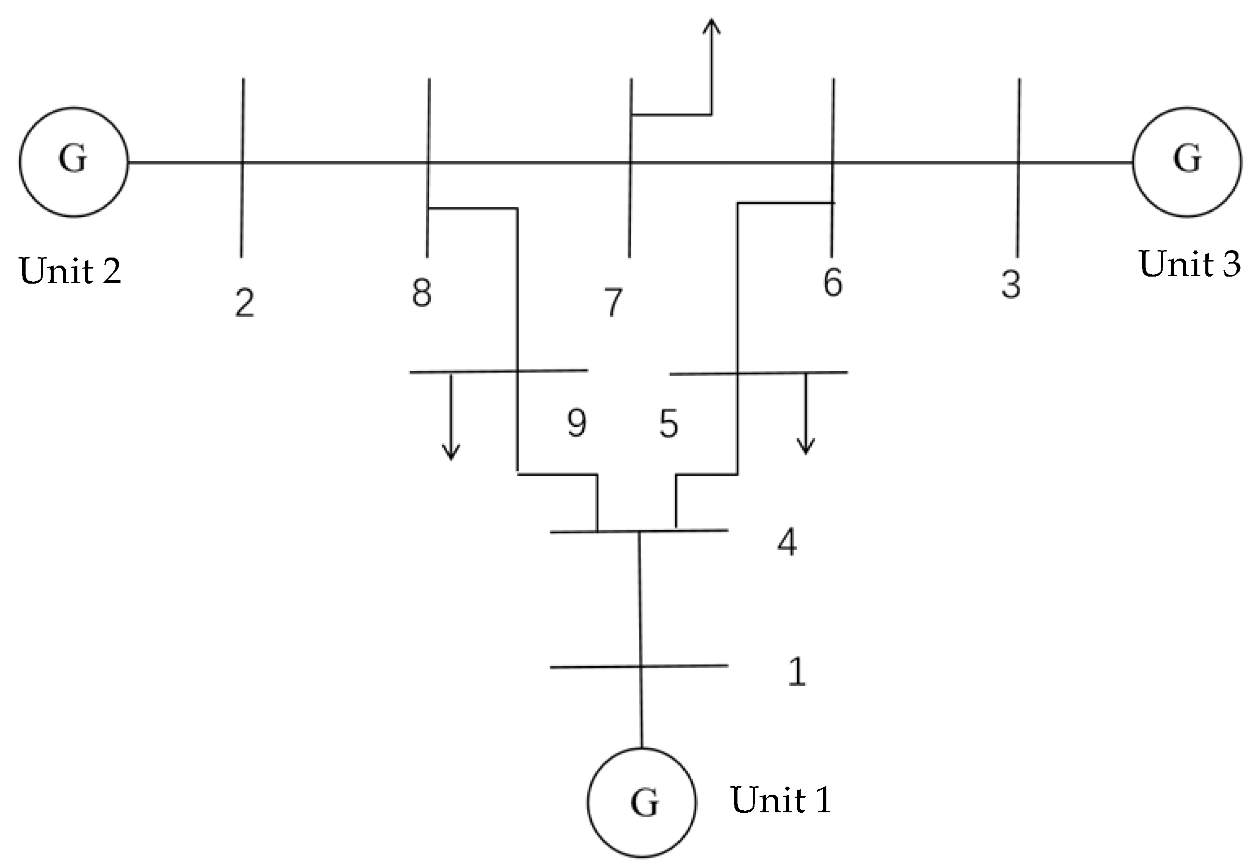
In this study, the DIgSILENT/Powerfactory (2022., DIgSILENT GmbH, Gomaringen, Germany) simulation platform is used to build a test system containing three synchronous generating units, nine bus nodes, and three load areas, and the system topology is shown in Figure 1. The system parameters are shown in Table 1. The simulation model is mainly used to verify the performance of the grid inertia assessment algorithm proposed in this paper, in which the key modeling parameters are related to the rated capacity of the generating units and the inertia time constant. The effectiveness of the proposed method for inertia assessment of synchronous generating units is confirmed by implementing the complete evaluation process and comparing and analyzing the results.
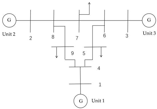
Figure 1.
WSCC 9-Bus System structural diagram.

Table 1.
WSCC 9-Bus System Simulation Parameters.
To validate the effectiveness of the technique suggested in this study, we first estimate the inertia of synchronous generators and compare the obtained results with the traditional inertia assessment method based on perturbation information. In the 3-machine, 9-node simulation system, the rated frequency is 50 Hz; the load distribution: 90/100/125 MW at nodes 5/7/9, respectively; 50% load surge is set on bus 5 at 2 s. The disturbance type is a load surge to simulate active power imbalance. Firstly, the quantity measurements of each generator port measured by PMU for each generator after the perturbation occurs are read, including the active power, reactive power, voltage magnitude and voltage phase angle, as well as the bus frequency, and the data window is selected to be 20 s. The simulation step is 0.01 s. The data window is selected to be 20 s, and the simulation step size is 0.01 s. The simulator is then used to estimate the inertia of the synchronous generator.
The measured data are shown in Figure 2:
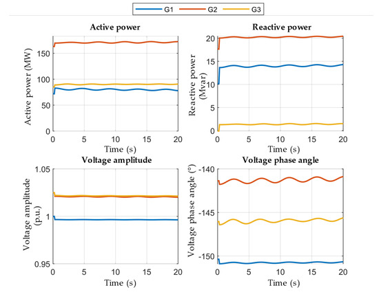
Figure 2.
Measurement data of WSCC 9-Bus System.
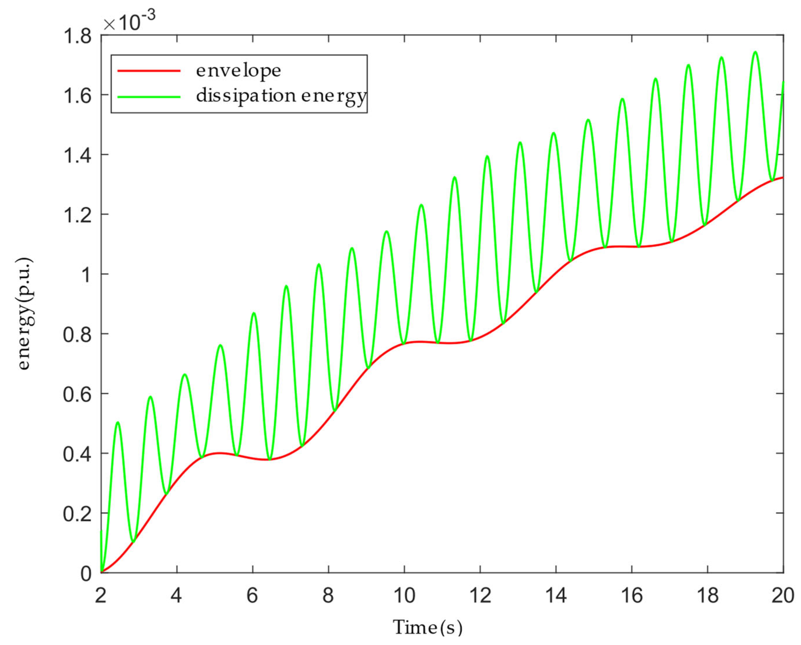
As can be seen in Figure 3 below, the dissipated energy at the generator port shows an upward trend, and its envelope satisfies the physical basis with the value of the damping term. The trend is approximated by the damping term, i.e., the envelope of the dissipated energy can be expressed as a damping term, and the contrast between the damping term and the envelope is shown in Figure 4:

Figure 3.
Dissipative energy and its envelope diagram.
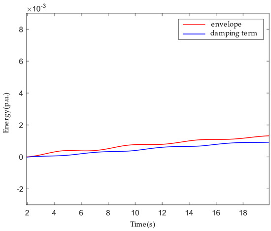
Figure 4.
Dissipative energy envelope and damping term.
Using the above calculation method, the inertia time constant H of the generating unit has been solved and analyzed by comparing the actual value with the evaluated value and compared with the traditional estimation method under the same perturbation, and the results are shown in Table 2.
Table 2.
Synchronous unit inertia assessment results.
According to the simulation results in Table 1, the frequency dynamic characteristics are mainly dominated by the inertial support effect in the initial stage after the system is subjected to perturbation. The inertia time constants of the unit calculated using the identification algorithm proposed in this paper are highly consistent with the actual parameters. Specifically, taking the G2 generating unit as an example, the relative deviation between the identification results and the actual values is only 0.59%, which fully verifies the excellent accuracy of the calculation method in the assessment of inertia parameters.
2.3.2. Impact of Damping Terms on Evaluation Accuracy
Under the same method, the results of G3 inertia evaluation with and without calculating the damping term are shown in Table 3.
Table 3.
Impact of damping terms on assessment results.
It can be seen that the damping term has an effect on the inertia evaluation results, and the error is very close when the damping torque coefficient is 1. At this time, the damping term has close to the minimum effect on the results. As the damping torque coefficient increases or decreases, the error with the results of the inertia assessment by the method of this paper is greater.
2.3.3. Stability Verification Under Large Perturbations
In order to verify the stability and accuracy of the energy function method under strong nonlinear scenarios, the following working conditions are designed: system conditions: the load level is raised to 120% of the rated load (close to the system stability limit), simulating a heavy load operation state. A three-phase short-circuit fault is applied at t = 1 s for 0.1 s to stimulate a strong transient response of the system. The traditional RoCoF method and the small-squares method are also used for the inertia assessment to compare the error characteristics (Table 4).
Table 4.
Inertia assessment error under heavy load short circuit conditions.
The relative error of the energy function method is only 0.91%, which is significantly lower than that of RoCoF (10.44%) and Least square (LS) (3.92%), proving its accuracy advantage in strong nonlinear scenarios. RoCoF, which relies on the rate of change of the frequency, is significantly affected by the high−frequency oscillations after the fault, and the error is enlarged; and LS, which assumes that the system is linear, is not able to adapt to the strong time-varying characteristics after the short-circuit fault, resulting in the estimation deviation of 120%. A three-phase short-circuit fault at rated load triggers strong nonlinearities in the electromechanical transient processes of the system (e.g., large oscillations of the generator power angle, risk of deep rotor out-of-step), and traditional methods based on the assumption of linearization (e.g., RoCoF, LS) are susceptible to estimation failures due to model mismatch.
Based on the global integral property of energy conservation, the inertia information is extracted directly from the port energy flow, avoiding the local linearization assumption. The transient energy is decomposed into inertia-dominated period term and damping-dominated decay term by the vibration mechanics envelope extraction technique, which suppresses the high-frequency noise generated by fault impact. The working condition verifies the reliability of the energy function method under the critical steady state of the system, which can provide technical support for the post-fault inertia assessment of new energy high penetration power grids.
3. Evaluation of the Inertia of Doubly Fed Turbines Taking into Account the Virtual Inertia of the Turbine
This part may be broken into subheadings. It should include a clear and succinct account of the experimental data, their interpretation, and the experimental inferences that may be inferred.
3.1. Evaluation Method of Doubly Fed Wind Turbine Inertia Assessment Based on Energy Function
The synchronous machine achieves electromechanical energy conversion through the coupling of rotor mechanical speed and power angle, and its inertia is directly determined by the rotor inertia. DFIG is controlled by a power electronic converter, and the rotor mechanical speed is decoupled from the grid frequency, so the traditional power angle is no longer applicable [34]. Its inertia needs to be simulated by virtual control to simulate the characteristics of the synchronous machine, so an equivalent power angle–energy conversion model needs to be established.
Based on the approach of building the synchronous generator energy function and the port energy function, the rotor of the wind turbine’s equation of motion may be expressed in the following linear incremental form:
After integrating both sides of the equation, we have
Doubly fed induction generators (DFIGs) differ fundamentally from synchronous generators in their dynamic characteristics. The mechanical speed of a synchronous generator is differentially related to the power angle, whereas the operating characteristics of a DFIG do not contain the conventionally defined power angle parameter due to the power electronic converter control. This characteristic difference leads to the fact that the electromechanical energy conversion relationship described in Equation (24) cannot be directly applied to the kinetic–potential energy conversion model of the synchronous generator [35]. To solve this problem, an equivalent power angle theoretical framework applicable to DFIGs is required.
Based on Thevenin’s theorem, the interaction of a grid-connected power generation device with the grid can be simplified to a circuit model with an equivalent AC voltage source in series impedance. Among them, the equivalent internal potential can effectively characterize the dynamic response properties of the device. By solving the electromagnetic equations (including the voltage balance equation and the magnetic chain conservation equation) of the DFIG in a synchronously rotating dq reference system, the mathematical expression of its equivalent internal potential can be obtained analytically. Since the DFIG lacks the power angle parameter in the traditional sense, its equivalent potential energy term must be reconstructed by energy dissipation analysis, which is crucial for an accurate description of its dynamic behavior.
According to Thevenin’s theorem, DFIG-grid-connected operation can be equated to a power supply with ‘internal potential E’ series equivalent impedance Zs’. Where: E’ reflects the combined effect of the dynamic response of the DFIG stator magnetic chain, whose amplitude and phase are determined by the rotor control strategy; the equivalent impedance Zs contains the converted values of stator leakage reactance and rotor excitation inductance. The DFIG under complex converter control is simplified to a ‘potential-impedance’ model similar to that of a synchronous machine, which lays the foundation for the definition of the equivalent power angle.
It can be obtained that Equation (27) is
Due to the relatively small generator stator time constant, the electromechanical transient analysis may ignore the generator stator’s transient process, yielding a reduced voltage phase equation:
Inductance is expressed as leakage inductance plus mutual inductance:
Thevenin’s theorem may be used to determine the equivalent circuit model of DFIG, where Us is the terminal voltage, and E′ is the equivalent internal potential of DFIG. The equivalent power angle δg may be used to establish the angle between the machine-end voltage Us and the equivalent internal potential E′ of the DFIG, as seen in Equation (28). When examined from a physical perspective, the DFIG’s equivalent power angle reflects the phase shift properties between the rotor and stator magnetic chain space vectors. It should be noted in particular that the dq reference system used for coordinate transformation in the DFIG control system is a virtual coordinate system established on the basis of the stator magnetic chain space vectors, instead of the traditional coordinate system definition based on the actual physical axes.
By analyzing the electromagnetic characteristics of the DFIG, it can be found that there is a significant mutual coupling between its stator and rotor magnetic chains. Especially in the transient condition, due to the influence of stator end voltage fluctuation, the rotor magnetic chain presents time-varying characteristics, which leads to the change of the equivalent internal potential with time. The mathematical link between the output power and the fluctuation of the equivalent power angle may be analyzed and determined by creating a correlation model between the DFIG’s power transfer characteristics and equivalent power angle characteristics, as shown in Equation (30):
The equivalent power angle δg is the phase difference between the DFIG equivalent internal potential E’ and the terminal voltage Us, and its physical meaning is that it reflects the spatial phase difference between the stator magnetic chain and the rotor magnetic chain, which determines the direction of electromagnetic power transmission, similar to the relationship between the power angle of synchronous machine and electromagnetic power. In the virtual inertia control, the dynamic change in δg simulates the inertial response of the rotor power angle of the synchronous machine.
After DFIG’s equivalent power angle is determined, it may be further deduced and obtained as follows:
The analytical derivation results show that DFIG exhibits a high degree of similarity with the synchronous generator in terms of the energy conversion mechanism by modeling the equivalent power angle. This similar feature enables the DFIG to be equivalently regarded as a special class of synchronous generators. In the mathematical model, Pe characterizes the electromagnetic power output from the DFIG, δg represents its equivalent power angle parameter, TJ describes the inertia time constant of the virtual synchronous control link, and ω reflects the angular velocity characteristics of the rotor rotation.
By analyzing the operation of in the integration interval δg1 to δg2, the mathematical expression can correspond to the increment of the mechanical power of the prime mover of the synchronous generator set. Similarly, the result of the calculation of in the same integration limit reflects the amount of change in the equivalent potential energy of the synchronous generator. Observing the difference in TJω22 between ω1 and ω2 states, this physical quantity characterizes the dynamic process of kinetic energy change in the rotor system. As far as the grid-side energy exchange is concerned, the integral operation of the intervals δg1 to δg2 with respect to can either be characterized by the port energy parameter or an approximate solution can be obtained by using the trapezoidal numerical integration method. Specifically, this discretization transforms the continuous integration into a segmented linear approximation, which significantly improves the computational efficiency while ensuring computational accuracy. Currently, the following expression may be used to describe the connection between the change in port energy and the changes in kinetic and potential energy within the port:
An estimate of the inertia time constant of the DFIG can be obtained from the above equation, see Equation (33):
In summary, this paper accomplishes the extraction of DFIG inertia time constants based on the energy function and realizes the estimation of wind turbine inertia for new energy power systems containing wind power.
The following are the settings for the simulation: the total simulation time is 100 s, and the sampling interval is 0.01 s to ensure the accurate capture of high-frequency dynamic processes. The load step perturbation of 225 MW is put into the simulation at 50 s to simulate the sudden power shortage scenario of the grid. DFIG control parameters: the virtual inertia gain coefficient Kvic is set to 1.2, the sag coefficient D is 0.8 p.u., and the allowable fluctuation range of the rotor speed is ±10% of the rated speed (i.e., 0.9–1.1 p.u.) to avoid triggering the over-speed protection.
3.2. Simulation Analysis
To evaluate the validity of the energy-function-based DFIG equivalent inertia time constant identification approach, this study designs a modified 3-machine 9-node system on the DIgSILENT/Powerfactory platform, replacing G3 (node 3) in Figure 1 with a DFIG and retaining G1 and G2 as synchronous machines. The system’s rated frequency is 50 Hz, voltage is 220 kV, and total capacity for load is 315 MW. The DFIG is connected to the grid via virtual inertia control, and it has a rated power of 128 MW. It includes a virtual inertia control module that simulates the synchronous machine’s inertia reaction and regulates the active output using RoCoF feedback. The inertia period constants for the synchronous generators SG1 and SG2 are set at 6 and 8 s, respectively, and the damping coefficient is 1.0 p.u. to simulate the FM characteristics of the conventional units.
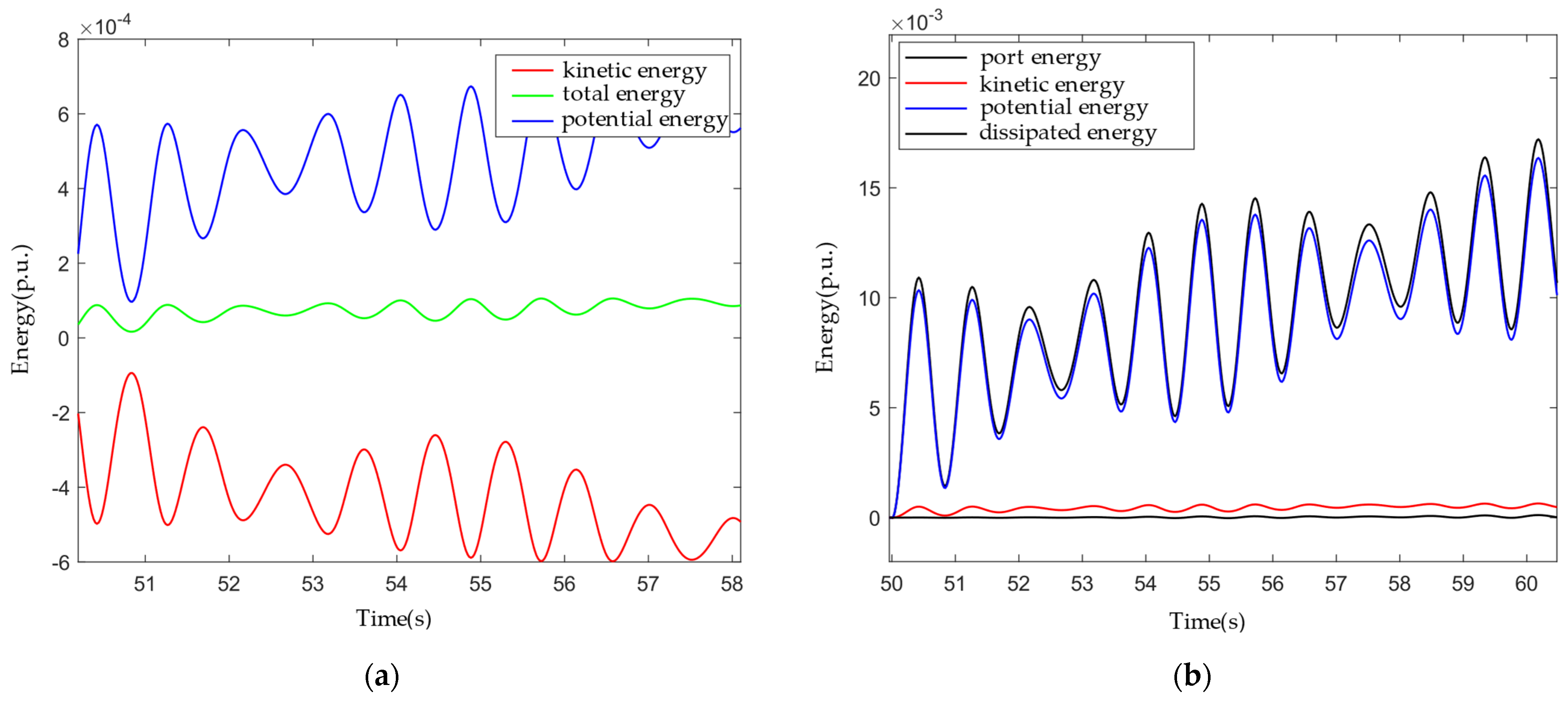
To verify the energy conservation, Figure 5 shows the transient energy dynamic balance process of DFIG under load disturbance (225 MW input at 50 s). The data in the figure were extracted by DIgSILENT simulation with a sampling interval of 0.01 s and the energy components were calculated by the trapezoidal integration method.
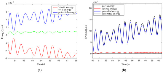
Figure 5.
Energy conservation verification of doubly fed induction generator with virtual inertia control: (a) total energy conservation curve; (b) dynamic decomposition of energy component.
This result further supports the rationality of the energy function method and provides a quantifiable analytical framework for the refined assessment of the inertia contribution of new energy units.
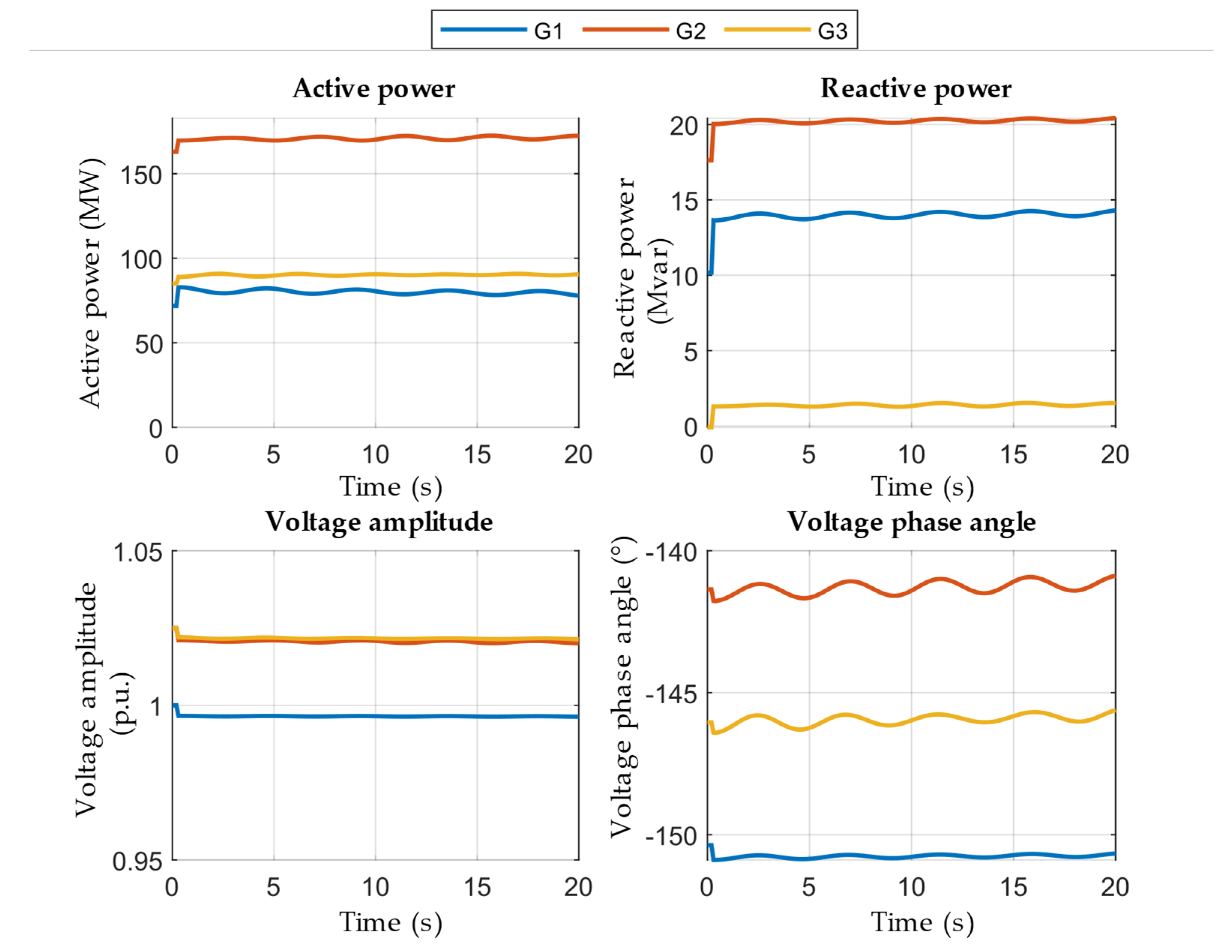
During the simulation process, the voltage phase angle, active power, reactive power, and equivalent power angle data of the DFIG port are collected, and the port energy function is calculated by the trapezoidal integration method, and the equivalent inertia time constant Hvsg is finally inverted based on the equation of conservation of energy. The quantity measurements are shown in Figure 6.
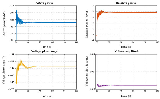
Figure 6.
Measurement of fan capacity in fan-containing systems.
In order to verify the generality of this paper’s method, the inertia time constants are estimated using this paper’s method, the traditional RoCoF-based inertia identification method, and the least squares method, respectively, and compared in this paper. The RoCoF method estimates the inertia by measuring the maximum rate of change of the frequency after a load perturbation; however, it is very sensitive to noise, and the error may be more than 15%, especially when the data fluctuate dramatically at the beginning of the perturbation (See Table 5). The least squares method estimates the inertia parameters by fitting the input and output data, and the recursive least squares method is used to identify the inertia constants of the virtual synchronous generator, but the method has limited ability to track the time-varying parameters and is susceptible to data saturation problems [17,18,19]. The comparison results are as follows:
Table 5.
Impact of damping terms on assessment results.
This method shows significant advantages in the virtual inertia evaluation of DFIG: firstly, it simplifies the parameter requirements by only collecting the power and voltage phase angle information of DFIG ports, without additional measurement of frequency or mechanical power parameters, which effectively reduces the cost of hardware and the communication burden; secondly, it has excellent noise immunity and can maintain a high accuracy even in the early stage of the disturbance when the data fluctuate strongly by integrating operation to smooth out high frequency noise; secondly, it has excellent noise resistance and can maintain a high accuracy even in the early stage of the disturbance when the data fluctuate strongly, and the phase of the perturbation can still maintain a high degree of accuracy; third, the introduction of vibration mechanics eliminates the effect of damping.
4. Conclusions
This study focuses on the problem of inertia assessment and proposes an energy-function-based inertia time constant identification method, which provides a new technical means for the frequency stability analysis of high-ratio new energy power systems. The study analyzes the differences in the inertia support process between synchronous generators and DFIGs through comparative analysis, reveals the physical nature of DFIGs simulating the dynamic response of synchronous machines through virtual inertia control, and proposes an inertia assessment method based on the energy function. Moreover, the study integrates the two frameworks and introduces vibrational mechanics to eliminate the influence of the damping term. In addition, combined with amplitude-phase dynamics, the relationship between the internal and external angles of the generator is analyzed, and the conclusions are introduced into the new energy unit. Simulation results show that the proposed method can effectively perform inertia assessment in systems with reduced inertia levels due to new energy access, which is superior to the traditional RoCoF method and provides a theoretical basis for further regional inertia level assessment, as well as system inertia assessment.
Author Contributions
Writing—original draft, S.W.; writing—review and editing, S.W. and Z.S. All authors have read and agreed to the published version of the manuscript.
Funding
This research received no external funding.
Data Availability Statement
The data that support the findings of this study are available from the corresponding author upon reasonable request.
Acknowledgments
The authors of this article thank the editorial department of the publisher and the School of Northeast Electric Power University of Technology for their strong support.
Conflicts of Interest
The authors declare no conflicts of interest.
References
- Li, S.; Deng, C.; Long, Z.; Zhou, Q.; Zheng, F. Calculation of equivalent virtual inertia time constant for wind farms. Autom. Electr. Power Syst. 2016, 40, 22–29. (In Chinese) [Google Scholar]
- Li, S.; Xu, S.; Li, H.; Shu, Z.; Huang, S.; Tian, B. A fast estimation method for equivalent virtual inertia of wind farms based on controlled autoregressive model. Power Syst. Technol. 2021, 45, 4683–4691. (In Chinese) [Google Scholar]
- Fu, Y.; Wang, Y.; Zhang, X.; Luo, Y. Analysis and comprehensive control of inertia and primary frequency regulation characteristics for variable-speed wind turbines. Proc. CSEE 2014, 34, 4706–4716. (In Chinese) [Google Scholar]
- Yao, J.; Zhao, L.; Liu, A.; Zhou, T.; Zeng, X. Frequency regulation of permanent magnet direct-drive wind turbines based on fuzzy PD control. Power Syst. Technol. 2014, 38, 3095–3102. (In Chinese) [Google Scholar]
- An, J.; Sheng, S.; Zhou, Y.; Shi, Y. Measurement data-based evaluation method for equivalent virtual inertia of wind farms. Power Syst. Technol. 2023, 47, 1819–1827. (In Chinese) [Google Scholar]
- Ma, Y.; Li, J.; Wang, Z.; Zhao, S.; Guo, R. Real-time regional equivalent inertia assessment method for renewable energy power systems based on measurement data. Trans. China Electrotech. Soc. 2024, 39, 5406–5415. (In Chinese) [Google Scholar]
- Zhang, L.; Xiong, Z.; Ye, J.; Cheng, L. Power system inertia assessment considering wind power uncertainty. Adv. Technol. Electr. Eng. Energy 2023, 42, 89–96. (In Chinese) [Google Scholar]
- Wen, M.; Tu, Z.; Wen, Y.; Huang, H.; Liu, X.; Tan, Y. Equivalent Inertia Prediction Method for Power Grid Systems with High Wind Power Penetration. Chinese Patent CN115017725A, 6 September 2022. [Google Scholar]
- Li, S.; Cao, R.; Lei, X.; Li, Z.; Liu, D. Equivalent inertia assessment method for DFIG considering reactive power control. Power Syst. Prot. Control 2023, 51, 45–53. (In Chinese) [Google Scholar]
- Zografos, D.; Ghandhari, M. Estimation of power system inertia. In Proceedings of the 2016 IEEE Power and Energy Society General Meeting (PESGM), Boston, MA, USA, 17–21 July 2016; pp. 1–5. [Google Scholar]
- Sun, H.; Xu, T.; Guo, Q.; Li, Y.; Lin, W.; Yi, J.; Li, W. Analysis of the UK “8·9” blackout and its implications for China’s power grid. Proc. CSEE 2019, 39, 6183–6192. (In Chinese) [Google Scholar]
- Australian Energy Market Operator. Preliminary Report—Black System Event in South Australia on 28 September 2016; AEMO: Melbourne, Australia, 2016. [Google Scholar]
- Li, Z.; Wu, X.; Zhuang, K.; Wang, L.; Miao, Y.; Li, B. Analysis and reflections on frequency characteristics of East China Grid during “9·19” Jinsu DC bipolar blocking accident. Autom. Electr. Power Syst. 2017, 41, 149–155. (In Chinese) [Google Scholar]
- Tan, B.; Zhao, J.; Netto, M.; Krishnan, W.; Terzija, V.; Zhang, Y. Power system inertia estimation: Review of methods and the impacts of converter-interfaced generations. Int. J. Electr. Power Energy Syst. 2022, 134, 107362. [Google Scholar] [CrossRef]
- Inoue, T.; Taniguchi, H.; Ikeguchi, Y.; Yoshida, K. Estimation of power system inertia constant and capacity of spinning-reserve support generators using measured frequency transients. IEEE Trans. Power Syst. 1997, 12, 136–143. [Google Scholar] [CrossRef]
- Heylen, E.; Teng, F.; Strbac, G. Challenges and opportunities of inertia estimation and forecasting in low-inertia power systems. Renew. Sustain. Energy Rev. 2021, 147, 111176. [Google Scholar] [CrossRef]
- Chassin, D.P.; Huang, Z.; Donnelly, M.K.; Hassler, C. Estimation of WECC system inertia using observed frequency transients. IEEE Trans. Power Syst. 2005, 20, 1190–1192. [Google Scholar] [CrossRef]
- Azizipanah-Abarghooee, R.; Malekpour, M.; Paolone, M.; Terzija, V. A new approach to the online estimation of the loss of generation size in power systems. IEEE Trans. Power Syst. 2018, 34, 2103–2113. [Google Scholar] [CrossRef]
- Wall, P.; Gonzalez-Longatt, F.; Terzija, V. Estimation of generator inertia available during a disturbance. In Proceedings of the 2012 IEEE Power and Energy Society General Meeting, San Diego, CA, USA, 22–26 July 2012; pp. 1–8. [Google Scholar]
- Anderson, P.M.; Mirheydar, M. A low-order system frequency response model. IEEE Trans. Power Syst. 1990, 5, 720–729. [Google Scholar] [CrossRef]
- Li, Z.; Tang, Y.; He, F.; Luo, W. Parameter identification method for synchronous generators based on time-frequency transformation. Proc. CSEE 2014, 34, 3202–3209. (In Chinese) [Google Scholar]
- Bai, K.; Song, P.; Wu, Y.; Li, Y.; Liu, P.; Gao, X. Parameter identification method for synchronous generators based on time-domain simulation load rejection test. Electr. Power 2011, 44, 6–10. (In Chinese) [Google Scholar]
- Yue, C.; Zhen, W.; Liu, B.; Ju, P. Arbitrary load rejection test method for synchronous generator parameters. High Volt. Eng. 2008, 34, 319–323. (In Chinese) [Google Scholar]
- Ashton, P.M.; Taylor, G.A.; Carter, A.M.; Bradley, M. Application of phasor measurement units to estimate power system inertial frequency response. In Proceedings of the 2013 IEEE Power & Energy Society General Meeting, Vancouver, BC, Canada, 21–25 July 2013; pp. 1–5. [Google Scholar]
- Wang, W.; Yao, W.; Chen, C.; Deng, X. Fast and accurate frequency response estimation for large power system disturbances using second derivative of frequency data. IEEE Trans. Power Syst. 2020, 35, 2483–2486. [Google Scholar] [CrossRef]
- Xia, T.; Zhang, H.; Gardner, R.; Bank, J. Wide-area frequency based event location estimation. In Proceedings of the 2007 IEEE Power Engineering Society General Meeting, Tampa, FL, USA, 24–28 June 2007; pp. 1–7. [Google Scholar]
- Ashton, P.M.; Saunders, C.S.; Taylor, G.A.; Carter, A.M. Inertia estimation of the GB power system using synchrophasor measurements. IEEE Trans. Power Syst. 2014, 30, 701–709. [Google Scholar] [CrossRef]
- Ge, Y.; Flueck, A.J.; Kim, D.K.; Ahn, J.B. Power system real-time event detection and associated data archival reduction based on synchrophasors. IEEE Trans. Smart Grid 2015, 6, 2088–2097. [Google Scholar] [CrossRef]
- Ahmadyar, A.S.; Riaz, S.; Verbič, G.; Riesz, J. Assessment of minimum inertia requirement for system frequency stability. In Proceedings of the 2016 IEEE International Conference on Power System Technology (POWERCON), Wollongong, Australia, 28 September–1 October 2016; pp. 1–6. [Google Scholar]
- Zografos, D.; Ghandhari, M. Estimation of power system inertia. In Proceedings of the 2017 19th International Conference on Intelligent System Application to Power Systems (ISAP), San Antonio, TX, USA, 17–20 September 2017; pp. 1–6. [Google Scholar]
- Dimoulias, S.C.; Kontis, E.O.; Papagiannis, G.K. Inertia estimation of synchronous devices: Review of available techniques and comparative assessment of conventional measurement-based approaches. Energies 2022, 15, 7767. [Google Scholar] [CrossRef]
- Shams, N.; Wall, P.; Terzija, V. Active power imbalance detection, size and location estimation using limited PMU measurements. IEEE Trans. Power Syst. 2018, 34, 1362–1372. [Google Scholar] [CrossRef]
- Sagar, V.; Jain, S.K. Estimation of Power System Inertia Using System Identification. In Proceedings of the 2019 IEEE Innovative Smart Grid Technologies—Asia (ISGT Asia), Chengdu, China, 21–24 May 2019; pp. 285–290. [Google Scholar] [CrossRef]
- Jamraspong, P.; Surinkaew, T.; Ngamroo, I.; Watanabe, M. Improving Inertia Estimation Accuracy Using an Adaptive Framework for Centre of Inertia Selection. In Proceedings of the 2025 13th International Electrical Engineering Congress (iEECON), Hua Hin, Thailand, 5–7 March 2025; pp. 1–6. [Google Scholar] [CrossRef]
- Li, Y.; Guo, S.; Ma, G.; Li, Z.; Yang, J.; Chen, Z. Dynamic Estimation of Load-Side Equivalent Inertia by Using Clustering Method. CPSS Trans. Power Electron. Appl. 2025, 10, 1–9. [Google Scholar] [CrossRef]


Disclaimer/Publisher’s Note: The statements, opinions and data contained in all publications are solely those of the individual author(s) and contributor(s) and not of MDPI and/or the editor(s). MDPI and/or the editor(s) disclaim responsibility for any injury to people or property resulting from any ideas, methods, instructions or products referred to in the content. |
© 2025 by the authors. Licensee MDPI, Basel, Switzerland. This article is an open access article distributed under the terms and conditions of the Creative Commons Attribution (CC BY) license (https://creativecommons.org/licenses/by/4.0/).