Energy Management of a Semi-Autonomous Truck Using a Blended Multiple Model Controller Based on Particle Swarm Optimization

Abstract

Recently, the electrification and automation of heavy-duty trucks has gained significant attention from both industry and academia, driven by new legislation introduced by the European Union. During a typical drive cycle, the mass of an urban service truck can vary substantially as waste is collected, yet most existing studies rely on a single controller with fixed gains. This limits the ability to adapt to mass changes and results in suboptimal energy usage. Within the framework of the EU-funded OBELICS and ESCALATE projects, this study proposes a novel control strategy for a semi-autonomous refuse truck. The approach combines a particle swarm optimization algorithm to determine optimal controller gains and a multiple model controller to adapt these gains dynamically based on real-time vehicle mass. The main objectives of the proposed method are to (i) optimize controller parameters, (ii) reduce overall energy consumption, and (iii) minimize speed tracking error. A cost function addressing these objectives is formulated for both autonomous and manual driving modes. The strategy is evaluated using a real-world drive cycle from Eskişehir City, Turkiye. Simulation results show that the proposed MMC-based method improves vehicle performance by $5.19\%$ in autonomous mode and $0.534\%$ in manual mode compared to traditional fixed-gain approaches.

1. Introduction

Heavy duty vehicles (HDVs) are responsible for 27% of the total carbon dioxide emissions caused by road traffic in Europe. These emissions have increased by 25% in the past 30 years and remain in incline in the absence of regulatory policies [1]. In 2019, the EU proposed a new legislation that targets to regulate the CO₂ emission of heavy duty vehicles to be reduced by 15% in 2025 and about 30% by the end of 2030 [2]. Consequently, city councils and municipalities are keen to electrify the range of commercial HDVs for municipal applications, from vans to trucks. Councils in major cities, such as in Nottingham, are replacing their old diesel refuse trucks with electric ones. This transition is meant to reduce the CO₂ emissions of the city around 52 t per year [3]. Additionally, there has been a push in recent times for automating garbage collection. This is due to the fact that the use of automation can further reduce energy consumption by ensuring more precise and consistent control of vehicle speed and acceleration, which minimizes unnecessary energy losses caused by human driving variability and improves adherence to optimal drive cycles. To support such precision and adaptability in control, recent research has increasingly turned to advanced computational methods, particularly nature-inspired AI algorithms, which offer promising capabilities for optimizing complex, dynamic systems like energy management in electric vehicles.

Nature-inspired AI algorithms have gained popularity in solving complex engineering problems due to their adaptability and convergence efficiency. Recent advances have focused on hybrid and swarm-based metaheuristics. Shaikh et al. [4,5,6,7,8] have demonstrated that improved variants of mayfly optimization, salp swarm, moth-flame optimization (MFO), the grey wolf optimizer (GWO), and hybrid MF-PSO algorithms can outperform traditional methods in clustering, power transmission line optimization, and parameter estimation. Although these techniques have not been widely applied to vehicle control yet, their strong performance in dynamic, multi-variable environments underscores their potential relevance to energy management in semi-autonomous vehicles. These nature-inspired algorithms provide a flexible foundation for developing advanced control strategies in electric vehicles. In particular, PSO and its variants are increasingly used in vehicle energy optimization tasks due to their simplicity and effectiveness.

Building upon this, recent research on electric and hybrid vehicles has increasingly focused on energy management strategies to improve efficiency and range. Various optimization techniques have been employed to enhance controller performance and reduce energy usage. For example, a novel method for modeling motor losses from efficiency maps using particle swarm optimization (PSO) is presented in [9]. Hu et al. [10] use a dynamic programming algorithm combined with a novel powertrain topology to minimize fuel consumption by balancing power usage between the engine and battery. Similarly, Hwang et al. [11] apply PSO for power distribution, and Du et al. [12] employ a multi-objective energy management system (EMS) to improve fuel economy. Zhang et al. [13] propose an adaptive EMS based on driving condition recognition, where key parameters are optimized using PSO. Valladolid et al. [14] show that optimizing driving patterns enhances state of charge and efficiency, particularly when speed variation is limited to a specific range. Chen et al. [15] use grey model and Markov chain methods to predict instantaneous power needs in a non-linear predictive control scheme, optimized through multi-objective programming. Further, Liang et al. [16] propose a four-layer EMS for dual-motor heavy-duty vehicles, targeting both dynamics and efficiency, while studies such as [17,18] address the impact of variable operating temperatures on torque distribution.

While optimization techniques enhance energy efficiency, they must be paired with adaptive control strategies that respond to system variability. One prominent approach is the multiple model controller (MMC), developed to address systems with significant parameter variation. MMCs have been applied in various domains since the 1970s, originally for filter banks [19] and later extended to adaptive control [20] and fault detection [21]. MMCs are typically categorized as either switching-based, where only one controller is active at a time, or blending-based, where control signals from all candidate controllers are combined [22]. Blending methods, in particular, have been shown to offer smoother control transitions and greater robustness.

Recent studies have applied MMC concepts to vehicle systems, albeit still in limited scope. Zengin et al. [23] develop multi-model adaptive control for multivariable systems, while Yingkai et al. [24] apply multi-model predictive control to unmanned surface vehicles, demonstrating improved path tracking. In automotive contexts, Liu et al. [25] use a multi-objective model predictive controller for adaptive cruise control (ACC), and Liang et al. [26] apply adaptive predictive control for path-following under low-adhesion conditions. Other studies have applied MMC to suspension systems [27], rollover prevention [28], and fault-tolerant control in quadrotors [29]. A model predictive MMC is used for longitudinal stability in in-wheel motor architectures [30] and generalized predictive control is proposed for 4WD electric vehicles [31].

Although these applications highlight the flexibility of MMCs, many lack integration across vehicle control domains or validation in real-world, mass-varying conditions. The present study addresses this gap by implementing a blended MMC approach tailored to the dynamic mass variation observed in urban electric service trucks. The proposed method dynamically adjusts controller gains optimized via PSO, offering an adaptive, multi-objective control strategy suited for real-time applications.

However, even with automation, electric service trucks face unique operational challenges that significantly affect their energy efficiency and drive performance. One of the key issues is the large variation in vehicle mass during a typical collection cycle, which can nearly double as waste is collected. This variation introduces nonlinear dynamics into the vehicle system, making it difficult to maintain optimal control using a conventional fixed-parameter controller. Fixed controllers do not adapt to changing vehicle loads, resulting in increased energy consumption, reduced range, and compromised tracking performance relative to the desired drive cycle. Such dynamic mass changes have a profound impact on both energy efficiency and control precision, yet they are neglected in conventional control strategies.

This work is, therefore, motivated by the urgent need for real-time, mass-adaptive control methods that can ensure optimal energy use and accurate drive cycle adherence in demanding, stop-start urban operations. Current energy management and control systems often rely on static vehicle models or assume fixed mass, which fails to reflect real-world conditions where payload changes dynamically.

This limitation affects a wide range of stakeholders as well such as fleet operators concerned with energy costs and vehicle range, municipal authorities aiming to meet sustainability and service efficiency targets, vehicle manufacturers and control system developers seeking scalable solutions for diverse operating conditions, and policy makers working to reduce transport-related emissions while supporting practical electrification pathways.

While this is clearly critical for urban collection vehicles, the challenge is equally relevant for the electrification of long-haul freight transport, where mass variability arises not just from partial loads or customer-specific routing, but also from the volume-to-weight trade-offs of transported goods. For instance, a vehicle might be operating below maximum weight capacity due to space-limited bulky items, or it may be fully loaded with dense cargo. In both cases, the mass characteristics significantly affect propulsion demand, energy efficiency, and regenerative braking behavior. As electrification expands across both urban and long-haul heavy-duty vehicle sectors, adaptive control strategies that respond to real-time payload conditions will become essential for maximizing efficiency and extending vehicle range.

This work is technically significant and timely, as cities scale up the deployment of electric service vehicles and face increasing pressure to achieve operational efficiency under real-world conditions involving variable payloads, frequent stops, and demanding drive cycles.

In line with the outlined challenges, this work seeks to address the following research question: How can control gains be optimized and adapted to account for significant payload variation in electric service trucks? In response to this question, a blended multiple model PI-controller approach is proposed, in which control gains are dynamically adapted based on real-time payload variation. The objective is to reduce energy consumption and improve adherence to the desired drive cycle throughout the collection route. The longitudinal dynamics of the electric vehicle are modeled, and the effectiveness of the proposed controller is evaluated through simulation in the sections that follow.

To implement this approach, a novel energy management strategy is developed that adjusts the controller parameters of the gas and brake pedals in response to changing vehicle mass, rather than relying on fixed gains. For each defined mass interval, optimal PI gains are computed using a particle swarm optimization (PSO) algorithm. These gains are then blended using a multiple model controller (MMC) framework, with a weighting strategy based on real-time payload estimation.

This paper is organized as follows. Section 2 deals with the dynamic model of the e-RT. Section 3 details the blended multiple model PI-controller approach. Section 4 presents the optimization problem formulation and the technique used to solve it. Section 5 introduces the case study as well as three test cases utilized in simulation studies for comparative analysis. Section 6 compiles the main simulation results and Section 7 summarizes the main conclusion that could be drawn in this work.

2. Mathematical Modeling of the e-RT

To carry out the simulations for the assessment of vehicle behavior under a drive cycle, a mathematical model of the electric truck is built in MATLAB/Simulink. The model combines the longitudinal dynamics of the truck with the E-powertrain consisting of the motor and battery. Additionally, a driver’s block is modeled, which acts as the main controller, taking various inputs from the vehicle to determine the pedal positions of the accelerator and brake pedals.

All the forces are considered in the vehicle model, and speed and acceleration are calculated. In the model, $\theta$ is the road slope in $\left[\mathrm{r}\mathrm{a}\mathrm{d}\right]$ and $m\left(t\right)$ is the total variable mass of the vehicle as a function of time in $\left[\mathrm{k}\mathrm{g}\right]$. The vehicle is subject to resistive forces such as rolling resistance $F_{rr}$, aerodynamic drag $F_w,$ and grade resistance $F_g$.

Rolling resistance force is given by Equation (1).

$$F_{rr}=m\left(t\right)g{f}_r\cos \left(\theta \right)$$

(1)

where $f_r$ is the coefficient of rolling resistance and g is the acceleration due to gravity in $\left[\mathrm{m}{\mathrm{s}}^{-2}\right]$. The force due to aerodynamic drag is formulated by Equation (2).

$$F_w={\displaystyle \frac{1}{2}}\rho A_f{C}_D{V}^2$$

(2)

where ρ is the air density $[\mathrm{k}\mathrm{g}/{\mathrm{m}}^3]$, $A_f$ is the frontal area of the truck $\left[{\mathrm{m}}^2\right]$, $C_D$ is the drag coefficient, and $V$ is the velocity of the truck in $[\mathrm{m}/\mathrm{s}]$.

Equation (3) presents the force due to road grade.

$$F_g=m\left(t\right)g\mathit{sin}\left(\theta \right)$$

(3)

The vehicle also experiences longitudinal tire force, $F_{Tr}$, during accelerating and braking. Therefore, Equation (4) formulates the overall longitudinal dynamics of the vehicle with variable mass.

$$m(t)\dot{V}+{\displaystyle \frac{dm\left(t\right)}{dt}}\mathsf{\Delta }V=F_{Tr}-(F_{rr}+F_w+F_g)$$

(4)

Noting that the change of mass happens at stops with zero speed, Equation (4) can be rewritten, as expressed by Equation (5).

$$m\left(t\right)\dot{V}=F_{Tr}-{(F}_{rr}+F_w+F_g)$$

(5)

Tires’ tractive and braking force (Equation (6)) is generated by the wheels torque, $T$. The torque is controlled through a mapping from the pedal position input u, as described in the following section, $T=u{T}_{max}$. The control input switches between the accelerator pedal position (APP) and the brake pedal position (BPP), depending on the driving condition. $T_{EM,max}$ and $T_{Brake,max}$ are the maximum allowable EM torque in acceleration and friction torque in brake, respectively. Therefore, $T_{EM}=u{T}_{EM,max}\left[\mathrm{N}\mathrm{m}\right]$ in acceleration and $T_{Brake}=u{T}_{Brake,max}\left[\mathrm{N}\mathrm{m}\right]$ in braking. $T_{EM}$ and $T_{Brake}$ are the electric machine torque and brake torque delivered to the powertrain and wheels of radius $R_W\left[\mathrm{m}\right]$, respectively. The powertrain transfer ratio is $N_{PT}$ and its efficiency is ${\eta }_{PT}$.

$$F_{Tr}={\displaystyle \frac{u}{R_W}}\left\{\begin{array}{c}{T}_{EM,max}{N}_{PT}{\eta }_{PT},APP\ge 0\\ T_{Brake,max},BPP\ge 0\end{array}\right.$$

(6)

The power output from the motor can be expressed as the product of the motor torque and the angular speed, ${\omega }_{EM}[\mathrm{r}\mathrm{a}\mathrm{d}/\mathrm{s}]$, of the motor given by Equation (7).

$${\omega }_{EM}=N_{PT}{\displaystyle \frac{V}{R_W}}$$

(7)

However, to calculate the output power of the battery, the power losses in the motor must be considered as well. Therefore, the energy consumption of the battery during the drive cycle is expressed as the integration of the power over time in Equation (8).

$$E=\int P_{B}dt=\int {\displaystyle \frac{T_{EM}{\omega }_{EM}}{{\eta }_{EM}}}dt$$

(8)

where ${\eta }_{EM}$ is the electric motor efficiency calculated based on the efficiency map.

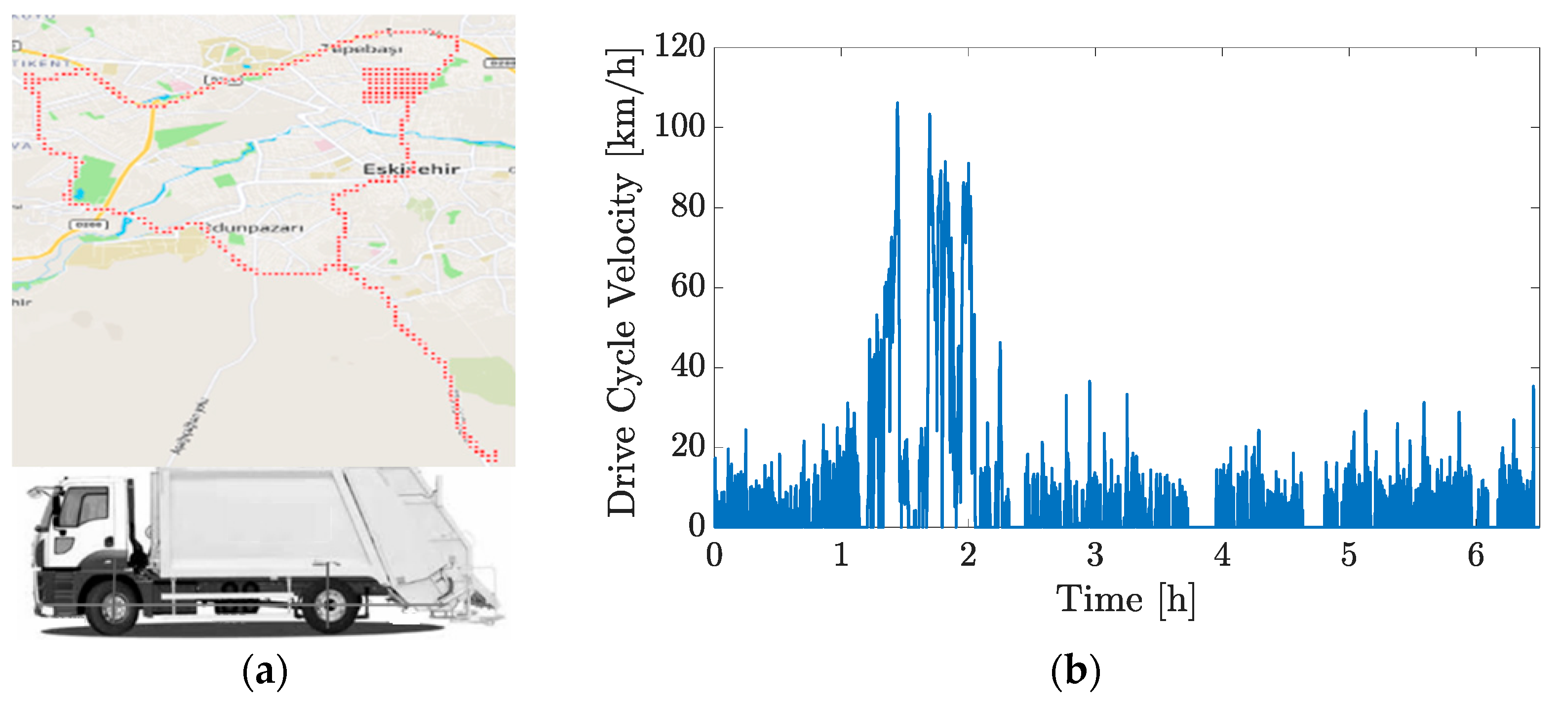
To carry out simulations to assess the behavior of the vehicle using the model elucidated in this section, it is important to emulate real-time variation of the vehicle mass within the vehicle model. Throughout its drive cycle, the vehicle mass increases from 9 t to 18 t. A variable mass model is designed which continuously increases the mass of the vehicle with time. A major factor in the design of the variable mass model is the fact that the vehicle mass only changes when the vehicle has stopped and is collecting waste. Thus, the variable mass model is designed to take inputs from the reference velocity cycle and garbage collection locations to determine the mass increase. Naturally, in real time, the vehicle weight would be measured using sensors or mass estimator filters and sent to the controller using the vehicle communication network.

3. Blended Multiple Model PI-Controller

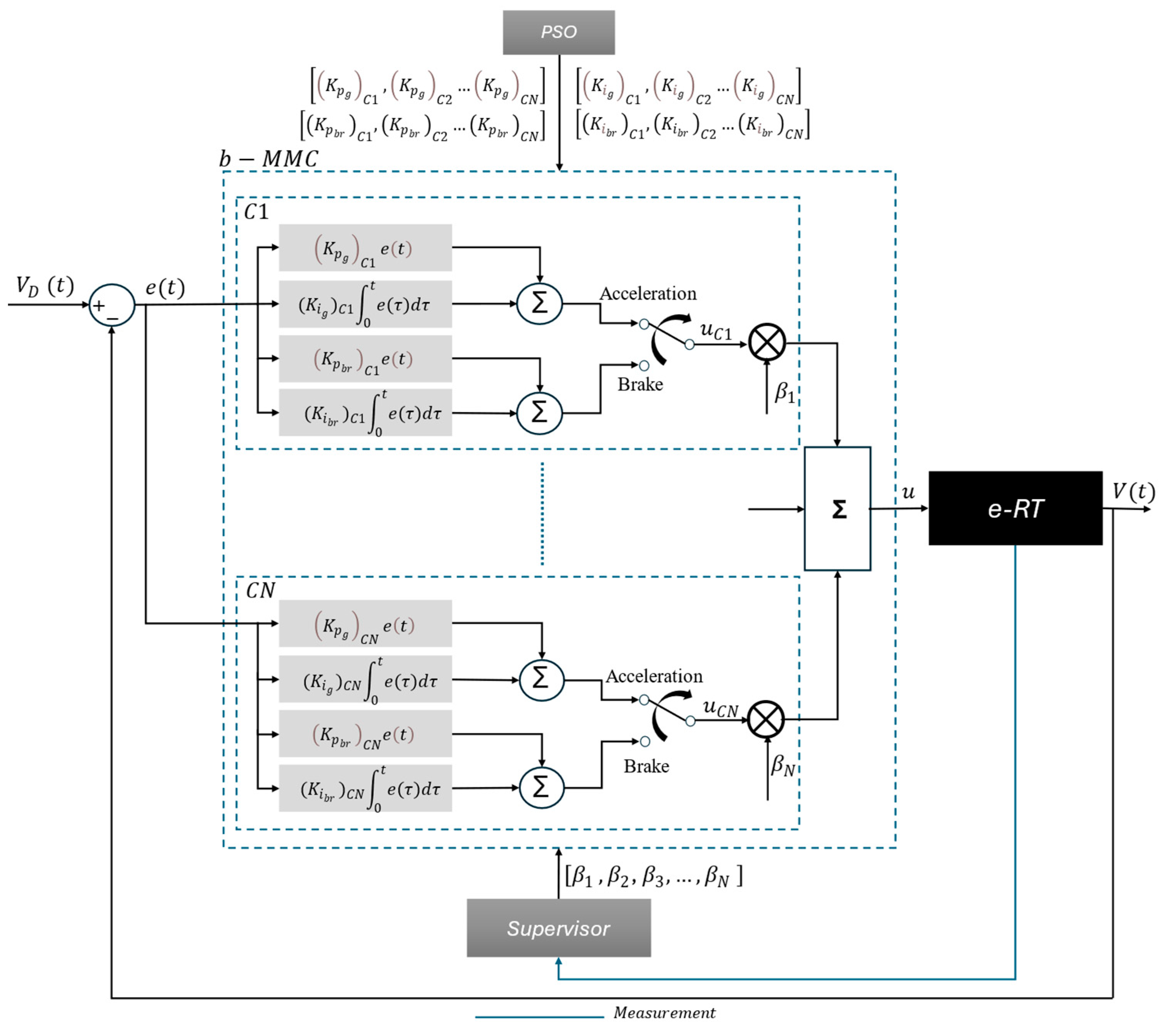
The blended multiple model control is an adaptive control strategy in which the controller parameters are modified online as the real-time conditions change. Multiple candidate controllers are assigned fixed parameters, and a supervisory controller assigns appropriate weights to each candidate based on feedback from the plant.

In this paper, the proposed technique consists of two sub-parts, the multiple model controller and optimization algorithm, which exchange optimal controller parameters depending on the existing payload and drive cycle. The payload of the refuse truck is assumed as a parametric uncertainty. A block diagram of the control strategy is shown in Figure 1.

In Figure 1, an error signal is generated from the input of the reference drive cycle and feedback of the plant model of the refuse truck. This error signal serves as the input to the main controller, which, in turn, calculates the optimal controller parameters for the accelerator and brake pedals using the bMMC (blended MMC) approach and PSO.

As a starting point in designing a multiple model controller, the maximum and the minimum values of the mass are defined. The range is separated into “$N$” number of subsets as in Equation (9).

$${\mathsf{\Omega }}_i=[a_i-b_i,a_i+b_i]$$

(9)

where $a_i$ and $b_i$ are design parameters that represent the limits of a subset ${\mathsf{\Omega }}_i$.

A candidate controller is assigned for each subset ${\mathsf{\Omega }}_i$ (Equation (10)). Therefore, “$N$” candidate controllers are assigned, as depicted in Figure 1. The output of each candidate controller is the summation of the proportional error and integration of the error signal, as shown in Equation (10). The first part of the controller reduces the steady-state error while enhancing the stability of the system, whereas the second part helps the controlled variable return to the exact set point following a disturbance.$.$

$$u_{Ci}=\left\{\begin{array}{c}{\left(K_{p_g}\right)}_{Ci}e\left(t\right)+{\left(K_{i_g}\right)}_{Ci}{\int }_0^{t}e\left(\tau \right)d\tau ,APP\ge 0\\ {\left(K_{p_{br}}\right)}_{Ci}e\left(t\right)+{\left(K_{i_{br}}\right)}_{Ci}{\int }_0^{t}e\left(\tau \right)d\tau ,BPP\ge 0\end{array}\right.$$

(10)

where the speed error from the refence drive cycle ($V_D$) is defined by $e\left(t\right)$. For each subset $Ci$, ${\left(K_{p_g}\right)}_{Ci}/{\left(K_{p_{br}}\right)}_{Ci}$ are the proportional gain constants and ${\left(K_{i_g}\right)}_{Ci}$/${\left(K_{i_{br}}\right)}_{Ci}$ are the integral gain constants for acceleration and brake, respectively. Therefore, $4\times N$ is the total number of controller gains to be defined through PSO.

After defining the subsets, candidate PI controllers corresponding to each subset ${\mathsf{\Omega }}_i$ are optimized offline using the PSO method to supply the necessary speed tracking performance and higher energy efficiency. The optimization algorithm is detailed in Section 4.

For the controller to adapt to the real-time conditions, information from the plant needs to be obtained to determine the subset in which the current mass of the vehicle is located. To enable this, a supervisor function is selected as in Equation (11).

$${\mu }_i\left(m\right)=\mu \left({\displaystyle \frac{m\left(t\right)-a_i}{b_i}}\right)$$

(11)

where $m\left(t\right)$ is the total mass as a function of time and $\mu$ is an exponential function expressed by Equation (12).

$$\mu \left(x\right)=\left\{\begin{array}{cc}\exp ({\displaystyle \frac{-1}{1-x^2}}+1),& \left|x\right|<1\\ 0,& \left|x\right|\ge 1\end{array}\right.$$

(12)

Subsequently, a weight function ${\beta }_i$, Equation (13), is employed to calculate the coefficients that determine the contribution of each candidate controller.

$${\beta }_i\left(m\right)={\displaystyle \frac{{\mu }_i\left(m\right)}{\sum _{k=1}^N{\mu }_k\left(m\right)}}$$

(13)

As depicted in Figure 1, the supervisor operates by measuring the real-time plant data and assigning the proper weights to each candidate controller.

Finally, the resulting blended control input of the system, accelerator, and brake pedal positions, is defined by Equation (14).

$$u={\sum }_{i=1}^N{u}_{Ci}{\beta }_i\left(m\right)$$

(14)

The blended multi model control strategy is designed to prevent possible undesirable transients and chattering caused due to sudden jumps between controllers. The overlap in the subsets serves as a region where the controller weights can be continuously varied to allow smooth switching from one subset to the other.

4. Optimization Approach

The optimization problem in this study combines two contradictory criteria and aims to strike a balance between them in a way that provides the best trade-off. The criteria in question are (i) the error between the reference and the actual velocity profile of the vehicle and (ii) the energy consumption of the truck. In an ideal case, both the velocity tracking error and energy should be minimized for the best performance; however, in the physical world, it is not possible to achieve this case. As the velocity tracking error decreases, the energy consumption of the truck rises and vice versa. Moreover, since the two entities are of different types, they are converted to dimensionless numbers and reduced to the same scale. Consequently, no one of the cost function components is dominating the other one. To formulate the cost function in an effective manner, it is important to understand the requirements of the vehicle to recognize the criterion at priority. Since the truck in development is semi-autonomous, it will have two modes of driving: manual and autonomous (Level 3). The requirements of the truck in each driving mode differ and, hence, the cost function is designed differently for each case.

For manual driving mode, an experienced driver will be operating the vehicle. In this case, the minimization of the energy consumption takes priority over the vehicle’s ability to track the longitudinal trajectory of the drive cycle. Hence, a lower weight is assigned to minimizing the tracking error of the vehicle. Contrary to this, in autonomous mode, the vehicle’s ability to track the longitudinal trajectory of the path takes higher priority than its energy consumption. This is to ensure that the vehicle stays on its designated speed profile and does not deviate from it. Hence, velocity tracking is assigned a higher weightage in this case of the operating condition. The optimization problem for each mass subset $Ci$ is formulated by Equation (15).

$$\begin{array}{c}\mathit{min}{\left\{J\left(K_{p_g},K_{i_g},K_{p_{br}},K_{i_{br}}\right)\right\}}_{Ci}\\ \\ {\left(K_{p_g},K_{i_g},K_{p_{br}},K_{i_{br}}\right)}_{Ci}\\ \\ s.t.:0\le {\left(K_{p_g}\right)}_{Ci}\le 150\\ \hspace{1em}\hspace{1em}0\le {\left(K_{i_g}\right)}_{Ci}\le 50\\ \hspace{1em}\hspace{1em}0\le {\left(K_{p_{br}}\right)}_{Ci}\le 200\\ \hspace{1em}\hspace{1em}0\le {\left(K_{i_{br}}\right)}_{Ci}\le 150\end{array}$$

(15)

where

$$J_{Ci}=\alpha \sqrt{\frac{1}{{\left(\mathsf{\Delta }T\right)}_{Ci}}{\int }_{{\left(T_{start}\right)}_{Ci}}^{{\left(T_{end}\right)}_{Ci}}{\left({V\left(t\right)}^{*}-V\left(t\right)\right)}^{2}dt}+\left(1-\alpha \right){\displaystyle \frac{{E\left(T_{end}\right)}_{Ci}-{E\left(T_{start}\right)}_{Ci}}{{\left(E_N\right)}_{Ci}}}$$

(16)

$J_{Ci}$ is the cost function, ${\left(\mathsf{\Delta }T\right)}_{Ci}={\left(T_{end}\right)}_{Ci}-{\left(T_{start}\right)}_{Ci}$, $\alpha$ is the weight of the tracking error root mean square (rms), ${V\left(t\right)}^{*}$ is the velocity of the reference drive cycle, $V\left(t\right)$ is the actual velocity of the vehicle, $E(.)$ is the total energy consumed, and $E_N$ is the energy normalization factor. The upper and lower bounds are defined based on reasonable controller signals. Optimization (15) can also be performed only once for the whole cycle as a single subset to find four control gains (one set rather than nine), which would be valid for the overall cycle. The optimization constraints bounds are defined based on the controller saturation limits. To prevent control signal oversaturation, the maximum allowable controller gains are determined such that, under worst-case conditions (e.g., maximum vehicle mass), the output does not exceed the saturation threshold of the control input. Notably, the resulting optimal values consistently fell within the final constraint bounds.

Particle swarm optimization (PSO) is an optimization technique that employs collaboration and exchange of information between individuals to find the optimum solution. In the classical model of the particle swarm optimization, a swarm of particles are initialized with a population of random solutions. The swarm particles parse through the dimension problem space to search new solutions with each subsequent iteration. Each swarm particle can be represented with a position vector and a velocity vector and is tasked with remembering its own best position. The best position is stored in a vector in every iteration. On the subsequent iteration, when the velocity vector is updated as shown in Equation (17), the swarm calculates and saves its new best position depending on its previous position and new velocity, given by Equation (18).

$${\overrightarrow{v}}_j=c_1\overrightarrow{v_j}+c_2\left(p_j-\overrightarrow{x_j}\right)+c_3\left(g_j-\overrightarrow{x_j}\right)$$

(17)

where, $p_j$, $g_j$, $\overrightarrow{x_j}$, $\overrightarrow{v_j}$, $c_1$, $c_2$, and $c_3$ are the swarm best fitness position, the particle fitness, the particle position, the particle velocity, the particle self-confidence, the particle confidence in its best performance, and the particle confidence in its best informant, respectively. $c_1$ is adaptively increasing with convergence and decreasing when the iterations diverge. $c_2$ and $c_3$ are uniformly distributed random numbers between 0 and 1.5.

The position of each particle in the swarm is updated by Equation (18).

$$\overrightarrow{x_j}\to \overrightarrow{x_j}+\overrightarrow{v_j}$$

(18)

This technique outperforms other intelligent optimization algorithms owing to its superiority in providing quicker convergence times and easy implementation, and it served as the chosen optimization strategy for this study.

To tune the cost function according to both manual and autonomous driving mode, a weight sweeping is performed to determine the most suitable bias in the minimization of energy consumption and velocity tracking error in both driving modes. Hence, optimization is performed for α = 0.1–0.9. Figure 2 shows the trend in the change of tracking error rms and energy consumption as the velocity tracking weight (α) increases.

For $\alpha \in \left[\mathrm{0.1\; 0.2}\right]$, the importance assigned to minimizing the energy consumption is so high that the vehicle is not able to meet the required drive cycle and the tracking error exceeds the acceptable limits, as depicted in Figure 2. Hence, the cost function for $\alpha \in \left[\mathrm{0.1\; 0.2}\right]$ is rejected and removed from further discussion. As a result, for manual and autonomous driving modes, $\alpha$ is assigned as $0.3$ and $0.9$, respectively.

5. Simulation-Based Case Study with Variable Payload Dynamics

A variable-mass truck provides an excellent platform to demonstrate the effectiveness of the proposed controller. Suitable candidates for implementation include vehicles from the Ford electric truck, which exhibit significant mass variation during operation. This real-world simulation based on a recorded drive cycle from Eskişehir City serves as a case study for evaluating the performance of the proposed bMMC-PSO strategy under realistic operating conditions.

Table 1. Ford truck’s parameters.

$\mathit{m}\left(\mathit{t}\right)\left[\times {10}^3\mathbf{k}\mathbf{g}\right]$	${\mathit{R}}_{\mathit{W}} \left[\mathbf{m}\right]$	${\mathit{A}}_{\mathit{f}} \left[{\mathbf{m}}^2\right]$	${\mathit{C}}_{\mathit{D}}$	${\mathit{f}}_{\mathit{r}}$	$\mathit{\rho } \left[\mathbf{k}\mathbf{g}/{\mathbf{m}}^3\right]$	$\mathit{g} \left[\mathbf{m}/{\mathbf{s}}^2\right]$
$9$–$18$	$0.5$	$9$	$0.7$	$0.006$	$1.18$	$9.81$

defines the Ford truck parameters used for this study. During the cycle, the Ford truck mass increases from 9 t to 18 t.

The drive cycle used in the case study and final simulations is a real-time recorded drive cycle of Eskisehir City in Turkiye, shown in Figure 3.

The number of candidate controllers is selected based on the truck’s payload variation range (9–18 t), divided into nine 1-tonne intervals, which results in nine mass subsets (N = 9) where ${\mathrm{a}}_{\mathrm{i}}\in \left\{9.5,10.5,\dots ,17.5\right\} \mathrm{t}$ and ${\mathrm{b}}_{\mathrm{i}}=0.5 \mathrm{t}$ (Equation (9)). This granularity ensures sufficient responsiveness to mass changes without introducing excessive complexity or computational cost. Further subdivision offers negligible gains in performance during preliminary testing and is, therefore, not pursued.

As shown in

Table 2. Overview of control strategy features for comparative analysis.

Test Case	Type	Controller Parameterization Strategy	Limitation	Objective Focus
1	Single + Fixed Gain	Expert Knowledge	Not Adaptable	Baseline Control Performance
2	Single + Fixed + Optimized Gain	PSO-based Optimization	Not Adaptable	Optimized Fixed-structure Performance Reference
3	Multiple + Optimized Gain	PSO-based Optimization per Mass Segment	Adaptable	Multi-objective Adaptive Control

, a comparison is provided among three control strategies evaluated in this study. This comparison framework highlights the added value of adaptivity and mass-awareness in controller design for energy-efficient heavy-duty vehicle operation.

The three test cases described in this section are structured to enable a clear and systematic comparison between different control strategies under identical conditions. Test Case 1 represents a baseline using a manually tuned fixed-gain controller, reflecting conventional practice. Test Case 2 incorporates an optimized fixed-gain controller, offering insight into the performance gains achievable through optimization alone. Test Case 3 applies the proposed bMMC approach, which adapts the controller gains dynamically based on real-time vehicle mass. This progression allows the effect of optimization and adaptivity to be independently assessed. The corresponding simulation results and performance comparisons are presented in detail in Section 6.

6. Results

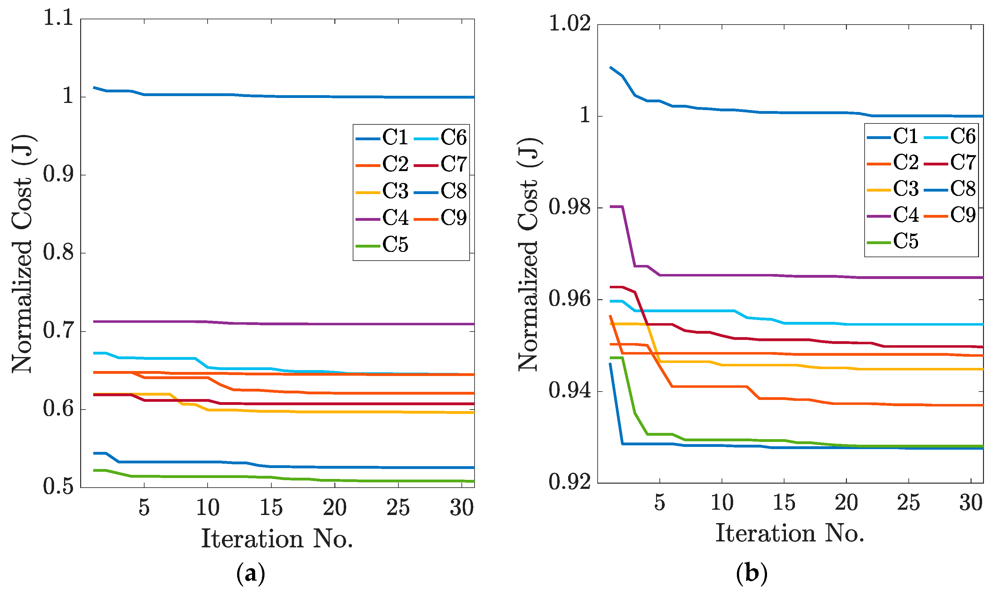
The optimization is performed offline to obtain the optimal controller gains for each candidate controller assigned to each subset of vehicle mass for both autonomous and manual driving modes. The drive cycle is also split into subsets corresponding to the subset of mass it overlaps with. The controller gains are optimized for only the subset in which the candidate controller lies, and not for the entire drive cycle. This reduced the simulation time by approximately 10 times. The convergence behavior of the PSO algorithm is illustrated in Figure 4a,b for both autonomous and manual driving modes, respectively, via the normalized progression of objective function values. The plots show a smooth and stable reduction in the cost function value, with convergence typically achieved well before the maximum number of iterations. This indicates that the optimization process is effective and does not suffer from premature stagnation or instability. The result reinforces the suitability of PSO for control parameter optimization in the proposed bMMC framework, even under varying payload conditions.

The convergence plot indicates that the algorithm approaches the optimal cost value effectively, with no significant improvement observed beyond the defined iteration limit.

Figure 5 shows controller gains for the gas and brake pedal with increase in the mass of the vehicle for both driving modes.

From Figure 5, it can be inferred that the integral controller gains in autonomous mode are higher than those in manual mode. This is because integral gains serve to reduce the steady state error of the system and since the minimization of velocity tracking error is prioritized in autonomous mode, higher integral gains are witnessed. For both driving modes, the proportional gains are comparable in magnitude and climb as the vehicle mass increases, which shows that a certain correlation lies between the proportional gains of the pedal controllers and the vehicle mass. The optimal values also have a correlation with the corresponding section of the drive cycle as well. In other words, if the truck of the same mass goes through a different speed profile, new optimal values should be sought.

The optimization results also show the minimum value of the cost function for each mass subset in both driving modes. The minimum cost values are normalized and plotted in Figure 6 to analyze the variation with increase in mass.

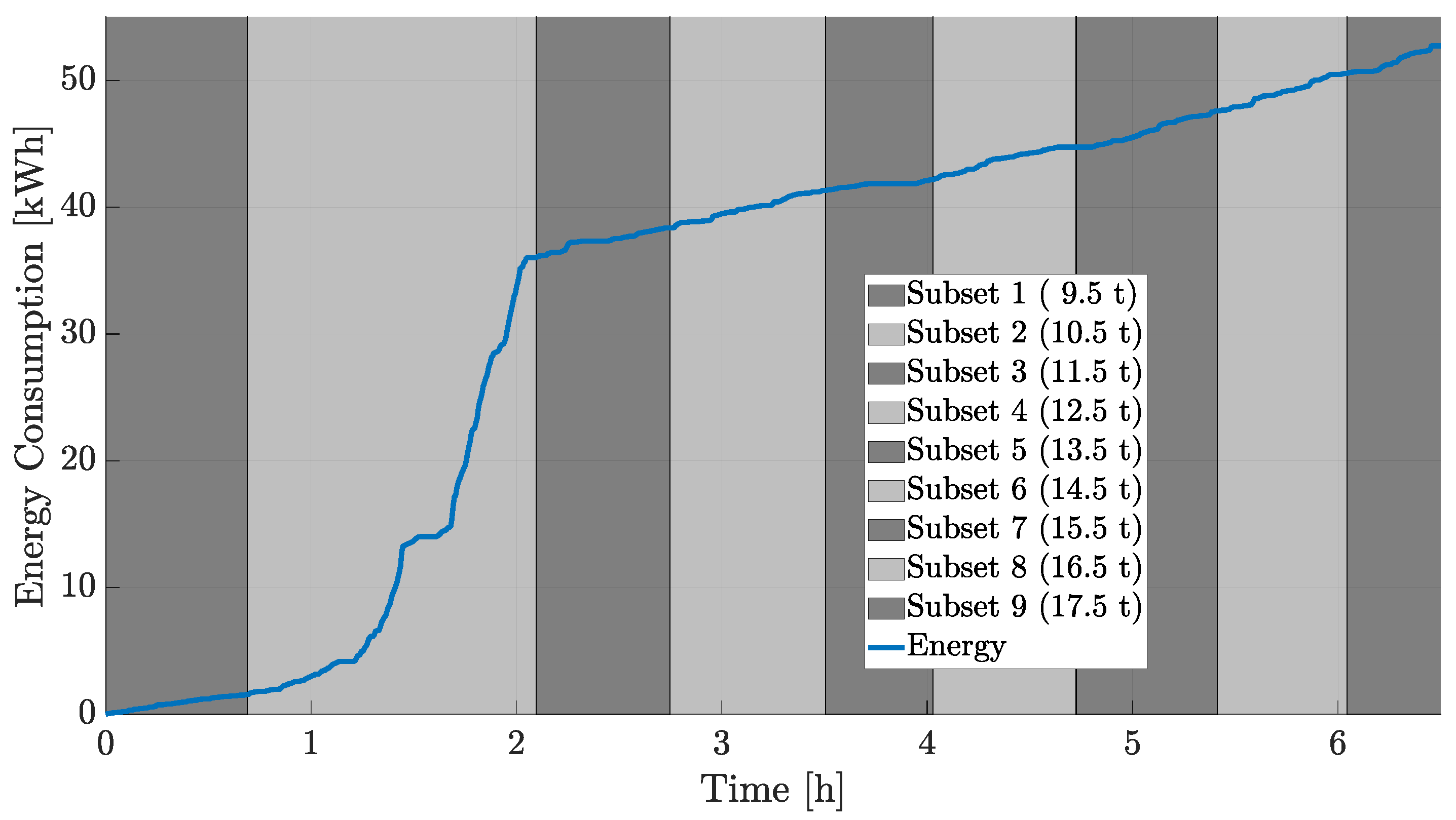
From Figure 6, it can be inferred that the cost values in both modes remained comparable, desirably, as the mass increased throughout the drive cycle. This can be explained by the fact that a decent normalization value, $E_N$, is selected for each subset. $E_N$ for each subset is selected as the energy consumption during the subset corresponding part of the cycle, as shown in Figure 7.

However, the range of optimum cost values for manual mode (Figure 6b) is more confined, since the energy consumption of the vehicle has more impact on the cost value in this mode.

On the other hand, since the velocity tracking error has more impact on the cost value in autonomous mode (Figure 6a), the optimum cost of this mode experiences higher fluctuations amplitude depending on the tracking error during each subset. The pattern of these fluctuations is yet visible in manual mode (Figure 6b) with a lower amplitude due to lower tracking weight, $\alpha$.

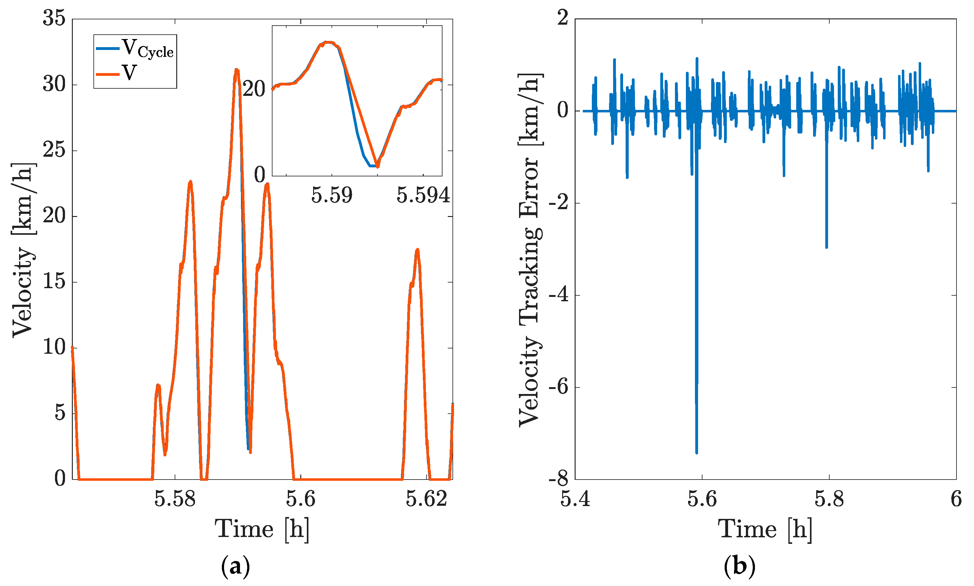
In both autonomous and manual driving modes, the cost value peaks for mass subset 8, as seen in Figure 6. Investigating this fact reveals that for the section of the drive cycle that corresponds to mass subset 8, a steep braking action without a full stop (positive jerk) occurs in the drive cycle (Figure 8a). The velocity tracking during this region is poor, due to which the absolute value of tracking error increases dramatically, as shown in Figure 8b. This sudden increase in the tracking error accounts for the increase in the cost value during this region.

After obtaining the optimal controller gains from the optimization algorithm, the gains are sent to the candidate controllers in the bMMC model. The simulation is performed for three test cases described as follows:

Test case 1: The simulation is performed with a single controller with fixed gains selected manually for best performance. This is assumed as the baseline controller.

Test case 2: The simulation is performed with a single controller with fixed gains selected through optimization over the entire drive cycle. This strategy can highlight the improvements made by multiple optimal controllers transitioning smoothly.

Test case 3: The simulation is performed with bMMC and adaptive gains selected through optimization over the entire drive cycle.

The results of the cost value for all three test cases are given in

Table 3. Simulation results for autonomous driving mode.

Test Case	Type	Gains	Cost Value (Normalized)
1	Single controller, unoptimized gains	$K_{p_g}=116.50$ $K_{i_g}=23.98$ $K_{p_{br}}=186.30$ $K_{i_{br}}=140.99$	$1$
2	Single controller, optimized gains	$K_{p_g}=66.46$ $K_{i_g}=36.73$ $K_{p_{br}}=100.19$ $K_{i_{br}}=93.50$	$0.42253$
3	bMMC, optimized gains	Adaptive gains Figure 5, Figure 6, Figure 7, Figure 8 and Figure 9 sets	$0.4017$

when the vehicle operates in autonomous mode and

Table 4. Simulation results for manual driving mode.

Test Case	Type	Gains	Cost Value (Normalized)
1	Single controller, unoptimized gains	$K_{p_g}=115.11$ $K_{i_g}=0$ $K_{p_{br}}=179.54$ $K_{i_{br}}=42.37$	$1$
2	Single controller, optimized gains	$K_{p_g}=69.43$ $K_{i_g}=15.22$ $K_{p_{br}}=81.51$ $K_{i_{br}}=57.17$	$0.49894$
3	bMMC, optimized gains	Adaptive gains Figure 5, Figure 6, Figure 7, Figure 8 and Figure 9 sets	$0.49629$

for manual mode. By using the bMMC model proposed in the study, a reduction of 148.94% and 5.19% is seen in the cost value compared to when a single controller is used with unoptimized and optimized gains, respectively, while the vehicle operates in autonomous mode (bMMC assumed the baseline for calculation).

As shown in Table 4, in the manual mode of operation, the proposed solution using bMMC allows the cost value to reduce by 101.5% and 0.534% when a single controller is used with unoptimized and optimized gains, respectively.

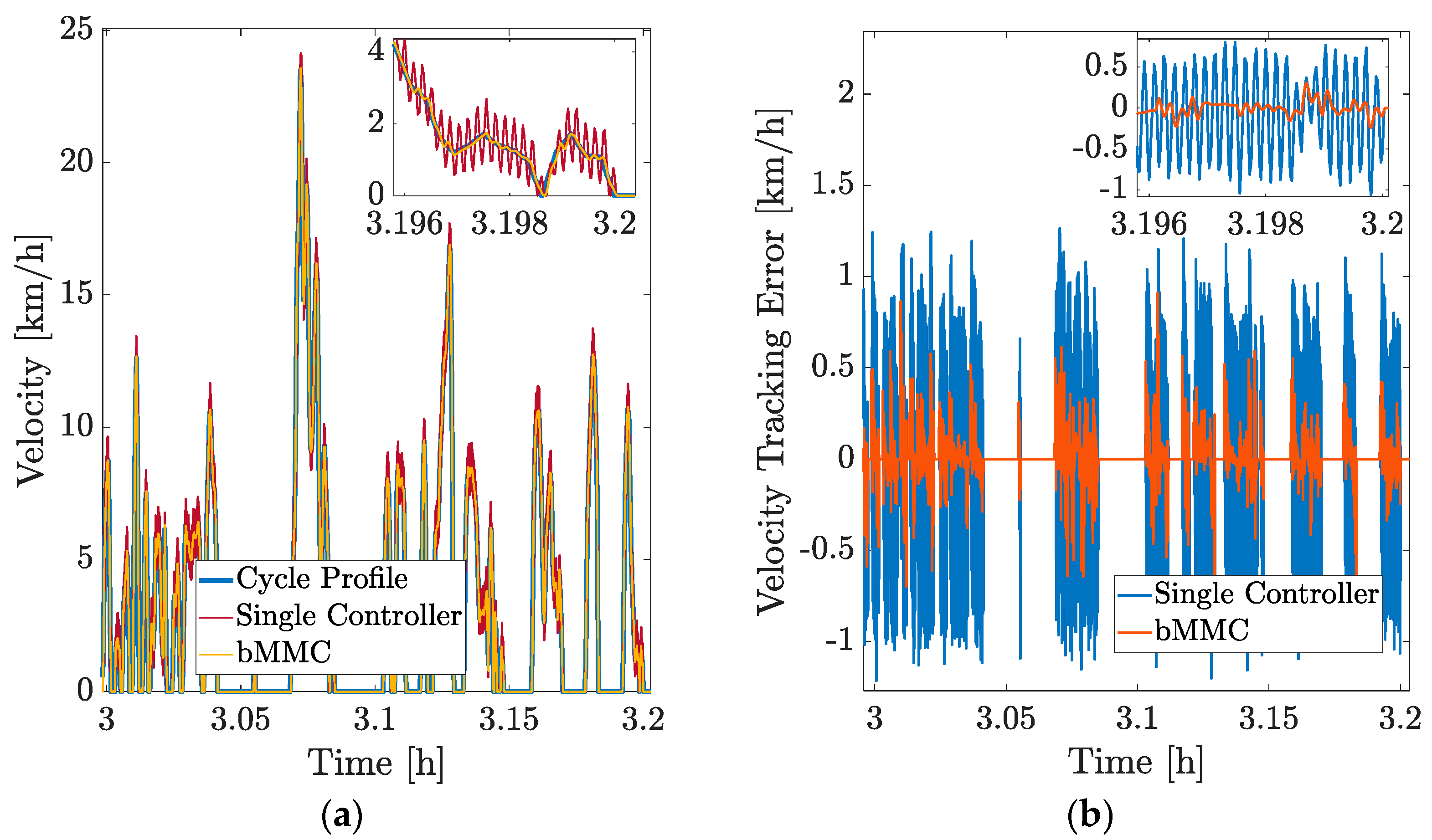
A clear improvement in the vehicle performance in terms of its energy consumption and velocity tracking ability is seen from the results. Moreover, the bMMC model is immune to large control input variations and its performance is robust in non-linear systems. This is important because the drive cycle input does not follow a linear trend and contains unpredictable variations. When such a non-linear input is given to a single controller, a lot of chattering is seen in the control output due to poor gain allocation. However, in bMMC, since the gains adapt themselves according to change in the control input, the output is smooth and does not contain any chatter, as shown in Figure 9.

Figure 9 shows the velocity profile of the vehicle using a single controller and bMMC and, as expected, a significant amount of chatter is seen when using the single controller. In this aspect, bMMC performs better than the existing approaches. Furthermore, Figure 9 also shows the difference in velocity tracking error while using a single controller and bMMC. In the former case, the velocity tracking error is approximately 200% higher than in the latter case.

7. Conclusions

In this paper, a novel adaptive control strategy based on blended multiple model control and particle swarm optimization is proposed to enhance the performance of autonomous refuse collection trucks in both autonomous and manual driving modes. In refuse collection application, the weight of the truck undergoes a significant variation throughout its drive cycle. Due to this, traditional control strategies employing a single controller that consider the vehicle weight constant are highly inefficient in optimizing the energy and velocity tracking ability of the vehicle. The design of the proposed control strategy is discussed and simulated for a real-time recorded drive cycle of Eskisehir city in Turkiye and compared with traditional approaches to show its superiority in refuse collection application. The results show that the performance of the vehicle improves by 5.19% in autonomous driving mode and 0.534% in manual driving mode. Moreover, since the system in question is highly non-linear in nature, single controllers with fixed gains show high chattering in the control output. The proposed bMMC strategy is robust against large control input variations and, hence, is suggested as the preferred method for refuse collection applications.

While this study focuses on a specific application scenario, the proposed bMMC-PSO strategy shows strong potential for broader use. Future work may extend this approach to include lateral dynamics control and evaluate its scalability across more diverse operating conditions. These developments would support the continued evolution of adaptive, energy-efficient control systems in real-world automated vehicle deployments.