Vortex-Induced Turbulence Optimized Membrane Enthalpy Exchanger: Dynamic Humidity Modulation and Coupled Heat–Mass Transfer Enhancement

Abstract

A bioinspired vortex-inducing architecture was engineered within the hydrodynamic focusing region of membrane-based enthalpy exchangers (MEEs) to generate controlled Kármán vortex shedding, strategically enhancing thermal–hygric coupling through boundary layer modulation. Computational simulations employing ANSYS Fluent 2024R1 and grid-convergence validation (GCI < 1.8%) demonstrated that at Re = 392 (2.57 m/s flow velocity), the vortex-integrated configuration achieved temperature exchange efficiency enhancements of 3.91% (summer) and 3.58% (winter), latent efficiency gains of 3.71% and 3.53%, alongside enthalpy effectiveness improvements of 3.37% and 3.36%, respectively. The interconnected momentum–heat–mass analogies culminated in peaks of performance evaluation criterion (PEC) = 1.33 (heat transfer) and 1.22 (mass transfer), substantiating vortex-induced Reynolds analogy optimization under typical HVAC operational scenarios (summer: 27 °C/50.3% RH; winter: 21 °C/39.7% RH).

1. Introduction

A considerable body of research has focused on air-to-air heat exchangers [1,2,3] in recent decades, driven by the evolving global energy consumption landscape. Reports indicate that building energy consumption accounts for a significant portion of total energy use and is a major contributor to carbon emissions [4]. In China, building energy consumption represents approximately 2% to 6% of total energy consumption [5]. Particularly in northern regions, heating energy consumption constitutes an even higher share of total building energy use. Among heating energy consumption, approximately 40% is lost due to factors such as building structure. The literature in [6] suggests that carbon emissions from building energy consumption contribute to 50% of total carbon emissions. Therefore, optimizing the building energy consumption structure is a critical step toward achieving carbon neutrality and realizing the dual-carbon economy, a sustainable strategic goal that benefits both the nation and its citizens.

Air-to-air heat exchangers are devices designed to recover energy lost in building energy consumption. Current research primarily focuses on enhancing the efficiency of energy recovery. Recently, studies have investigated the performance of air-to-air heat exchangers using various heat exchange materials [1,7,8]. These studies have shown that MEEs offer superior cost–performance ratios. A considerable body of literature has been published on MEEs [3,9,10,11,12,13]. While structural optimization strategies for microchannel heat exchangers are well documented [14,15,16,17], membrane-mediated thermal–hygric coupling in MEEs imposes fundamentally distinct constraints. Specifically, the semi-permeable membrane materials (e.g., selective water vapor transport layers) employed in MEEs require controlled, low-velocity flows to achieve optimal moisture transport, preventing membrane degradation and maintaining high hygric performance.

In addition, efforts have been made to optimize the structural design of heat exchangers. For instance, Zhang [18] optimized the structure of an MEE using the Number of Transfer Units (NTUS) method, achieving a design with optimal performance. Valerii I. Deshko [19] and colleagues compared numerical models of heat transfer in parallel plate channels with and without fins under varying wall temperatures. Neda Asasian-Kolur [20] and her team reviewed the performance of an MEE under different flow channel configurations, including cross-flow, quasi-counterflow, and triangular structures. Previous studies have explored various pin fin geometries for turbulence induction, including square [21,22] and elliptical [23] configurations. Square structures, while effective in creating flow separation at higher Re (>500), suffer from excessive pressure drop penalties in MEE conditions due to sharp-edge recirculation zones. Elliptical profiles demonstrate reduced form drag, but their orientation-dependent vortex shedding characteristics complicate manufacturability in thin (<0.1 mm) membrane spacers. In contrast, cylindrical structures exhibit axisymmetric flow separation that generates predictable Kármán vortex streets even at Re < 400 [24,25], making them particularly suitable for MEE’s spatially constrained, low-inertia flows. The cylindrical vortex-inducing elements (diameter d = 0.3 mm, pitch L = 10 mm) were dimensioned based on two-phase optimization criteria: Vortex Interaction Length Scale, where the L/d ratio (~33) exceeds the critical value of 20 required for full vortex street development in confined channels, ensuring that coherent vortices persist downstream [26]. Blockage Ratio Control [27]: with a channel height H = 2.5 mm, the 12% blockage ratio (d/H) minimizes permanent recirculation zones while maintaining sufficient momentum injection to disrupt concentration boundary layers.

In contemporary development efforts, a variety of research methods have been employed. Among these, numerical simulation techniques provide high-fidelity predictions of device performance. Many research institutions now use digital tools to accelerate development and reduce testing costs for MEEs. Commonly employed methods include finite element analysis [28,29], effectiveness-NTU methods [30,31,32], and computational fluid dynamics (CFD) modeling [2,7,8,11]. This study primarily utilizes CFD simulation software Fluent from the ANSYS commercial software package to conduct the simulations. The structural optimization of the air channels in an MEE is performed, and performance predictions are made using CFD tools. The theory of flow–solid coupling, which enhances heat transfer in microchannels, has been extensively applied in microchannel heat sinks for electronic equipment cooling [14]. Qing-wen Li [15] and colleagues simulated two types of intermittent microchannel configurations: straight and staggered. The results indicated that staggered microchannels exhibited the lowest thermal resistance and the highest friction factor, while continuous microchannels demonstrated the opposite performance. Yifan Li [16] and co-authors conducted numerical studies on the heat dissipation performance of microchannels combined with micro pin fins using a 3D conjugate heat transfer model, revealing the coupled mechanisms between fluid flow and heat transfer. Prabhakar Bhandari [17] numerically investigated the heat transfer and fluid flow characteristics of open microchannel heat sinks with square pin fins, predicting the performance of the devices. To date, a substantial body of the literature has focused on structural optimization for heat transfer enhancement, including pin fin configurations such as square [21,22], circular [33,34], water wing [21,35], elliptical [35], and others. In the case of MEEs, the Reynolds number (Re) is significantly lower than 2300 (with Re below 300 under the conditions described later in this study), indicating a fully developed laminar flow structure within the fluid domain. Therefore, to enhance both heat and mass transfer, it is essential to disrupt the laminar flow structure and induce turbulence.

In this study, a simplified CFD model was initially developed to verify the mesh-independent solution and compare it with experimental test data. The experimental data were used to validate the effectiveness of the CFD model and quantify the distribution of physical fields within the model. Subsequently, theoretical analysis revealed that introducing disturbance structures in the x- or y-direction within the fully developed laminar flow domain can effectively induce turbulence, specifically Kármán vortex street flow, thereby enhancing heat and mass transfer in microchannels. The physical field distribution and heat–mass transfer characteristics within the MEE were then visualized to elucidate the enhancement mechanisms. To our knowledge, this represents the first systematic demonstration of bioinspired cylindrical vortex generators in low-Re MEE environments. Unlike previous flow disruption strategies focusing solely on heat transfer enhancement [21,22,33,34], our approach explicitly addresses coupled thermal–hygric transport through synchronized vortex-induced boundary layer renewal as a critical mechanism for latent heat recovery optimization in membrane-based systems. Finally, the resistance distribution and efficiency balance of the MEE provided insights into potential research directions, with future work targeting the multi-objective optimization of variable geometries and materials—including scale-up strategies for full-size ERV cores through modular multi-cell array configurations, geometry ratio scaling (L/D = 5–30), and ΔP management under industrial airflow rates (1–3 m/s)—alongside integrating dynamic sorption hysteresis measurements into a multiscale CFD framework to couple vortex-enhanced transport with non-equilibrium sorption effects, with the findings offering significant implications for further understanding the principles of heat and mass transfer enhancement for sustainable HVAC systems.

2. CFD Model

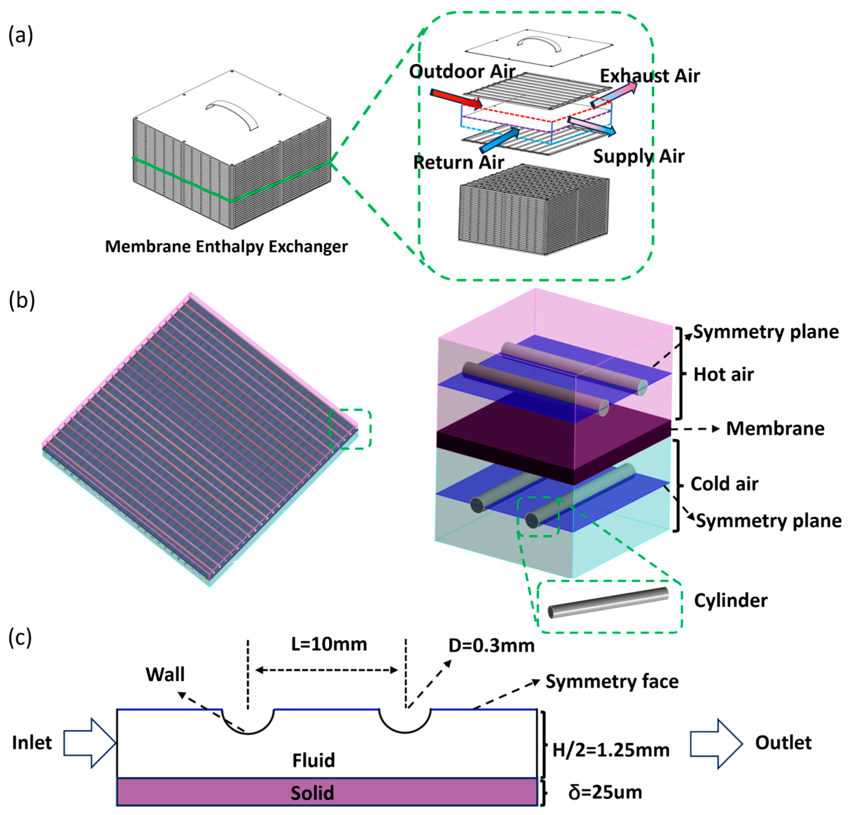
The subject of this study is the MEE device, as illustrated in Figure 1a. The device primarily consists of an injection-molded support structure made of Acrylonitrile–butadiene–styrene (ABS) material and a high-performance permeable polymer membrane from Fortuneway Technologies Inc. (Zhongshan, China), which functions as the thermal and humidity management medium for the enthalpy heat exchanger. A simplified schematic of the equivalent structure is shown in Figure 1b. For the purposes of modeling, the two adjacent airflow channels are referred to as the cold and hot channels, and the entire system is represented by an equivalent model. The model is divided into three layers: the upper layer represents the hot fluid, the middle layer represents the solid membrane material, and the lower layer represents the cold fluid, with the two fluids arranged in a cross-flow configuration. The operating conditions of the enthalpy heat exchanger, which constitute the primary focus of this simulation, include flow rates of 150 m³/h, 200 m³/h, 250 m³/h, 300 m³/h, and 350 m³/h.

2.1. Assumptions

For enthalpy exchangers, two primary technical strategies are commonly employed to enhance exchange efficiency: structural optimization and the selection of isolation materials. The choice of isolation layer material is crucial, as it influences both the heat and mass transfer efficiency of the exchanger and plays a key role in ensuring the long-term hygiene and effective operation of the air system. Common isolation materials can be categorized into paper-based and polymer materials. There is an extensive amount of literature that demonstrates that MEEs offer longer lifespans, lower degradation rates, and superior heat and mass transfer efficiencies [1]. Among these materials, the mass transfer behavior of polymers is particularly complex and warrants in-depth investigation. S. Koester [36] and colleagues investigated selectively permeable polymer membranes used in enthalpy exchangers. Their findings indicated that the gas permeation efficiency of membrane materials is primarily determined by two key parameters: selectivity and permeability. Selectivity depends largely on the physicochemical properties of the selective polymer layer, while permeability is influenced by the fluid dynamics near the membrane interface. Therefore, studying the dynamic behavior of enthalpy exchangers is critical, and this study focuses on the dynamics of these devices.

It is essential to simplify or omit certain details that have minimal impact on the actual results. These simplifications, though seemingly minor, are grounded in significant insights derived from the extensive research efforts of previous scholars. The key assumptions made in this study are as follows:

• Heat and mass transfer processes are assumed to be steady-state.
• The transport of water vapor through the membrane material is modeled as an adsorption–diffusion–desorption process, which is assumed to be in dynamic equilibrium. While adsorption/desorption hysteresis may modulate sorption capacity under transient conditions [37], its effects are excluded here due to the steady-state assumption of a simplification validated for isolating vortex-enhanced transport mechanisms [38]. Additionally, the latent heat of vaporization and adsorption heat on both sides of the membrane are assumed to be equal.
• Given the small temperature and water vapor concentration differences across the membrane, the thermal and moisture resistance within the membrane is assumed to be constant, with isotropic and constant thermal conductivity and diffusion coefficient for water vapor [8,12,29,39].
• The heat and mass transfer process within the entire enthalpy exchanger is simplified as the thermal and material exchange between two adjacent fluid channels.
• Solid surfaces are modeled using no-slip boundary conditions. In the equivalent model, the laminar flow model is employed to solve the equations, whereas the standard κ-ε turbulence model is used in the optimized model to enhance wall treatment.

2.2. Governing Equations

Currently, a wide range of commercial CFD software is available, with an extensive amount of the literature reporting on the simulation of heat exchangers using Fluent and the simulation of heat and mass transfer behaviors in enthalpy exchangers using COMSOL, among others. In this study, ANSYS Fluent 2024R1 is employed to simulate the heat and mass transfer processes in air-to-air MEEs. Although the Fluent solver efficiently handles fluid–solid coupling for heat transfer, it lacks a dedicated module for simulating the mass transfer process in MEEs. Therefore, this study utilizes Fluent’s user-defined function (UDF) feature [40] to implement mass transfer coupling simulations based on the actual operating conditions of the model. This paper focuses on examining heat and mass transfer behavior under both laminar flow and forced turbulence conditions.

2.2.1. Laminar Flow

In the current version of Fluent software [40], the general form of the governing equations for fluid–solid-coupled heat and mass transfer is presented in Equation (1). The first term on the lefthand side represents the transient term, while the second term represents the convective term. On the righthand side, the first term corresponds to the diffusion term, and the second term represents the source term. By solving Equation (1), the continuity equation is obtained, as shown in Equation (2).

$${\displaystyle \frac{\mathit{\partial }\rho \varphi }{\mathit{\partial }t}}+\nabla \cdot \left(\rho \varphi \overrightarrow{\mathrm{V}}\right)=\nabla ·\left({\Gamma }_{\varphi }{\nabla }_{\varphi }\right)+{\mathrm{S}}_{\varphi }$$

(1)

$${\displaystyle \frac{\mathit{\partial }\rho }{\mathit{\partial }t}}+\nabla \cdot \left(\rho \overrightarrow{\mathrm{V}}\right)=0$$

(2)

For incompressible gases, the density ρ is assumed to be constant, allowing the equation to be simplified as follows:

$$\nabla \cdot \left(\rho \overrightarrow{\mathrm{V}}\right)=0$$

(3)

$$\nabla \cdot \left(\rho \overrightarrow{\mathrm{V}}{\mathrm{Y}}_i\right)=\nabla ·{\overrightarrow{\mathrm{J}}}_i$$

(4)

By solving the continuity equation (Equation (3)) and the multi-species transport equations (Equation (4)), the mass distribution of multiple species within the fluid domain can be determined. The temperature field distribution is obtained by solving the energy equation (Equation (5)).

$$\nabla \cdot \left(\overrightarrow{\mathrm{V}}\left(\rho \mathrm{E}+\mathrm{P}\right)\right)=\nabla ·\left(k\nabla \mathrm{T}-\sum _i{h}_i{\overrightarrow{\mathrm{J}}}_i\right)$$

(5)

According to the literature [41], during the adsorption and desorption processes of water vapor on both sides of the membrane, the latent heat of vaporization and the latent heat of adsorption are equal in magnitude but opposite in direction. Therefore, Equation (5) can be simplified as follows:

$$\nabla \cdot \left(\overrightarrow{\mathrm{V}}\left(\rho \mathrm{E}+\mathrm{P}\right)\right)=\nabla ·\left(k\nabla \mathrm{T}\right)$$

(6)

In the above equation, k represents thermal conductivity, T denotes the temperature of the humid air, ${\mathrm{Y}}_i$ is the mass fraction of species i, and ${\overrightarrow{\mathrm{J}}}_i$ is the diffusion flux of species i. The diffusion flux of species i (either air or water vapor) increases with the concentration gradient. By default, the dilute approximation is employed. Under laminar flow conditions, the diffusion flux is described by the following equation (Equation (7)):

$${\overrightarrow{\mathrm{J}}}_i=-\rho {\mathrm{D}}_{i,ma}\nabla {\mathrm{Y}}_i$$

(7)

${\mathrm{D}}_{i,ma}$ is the mass diffusion coefficient of species i (m²/s), which is defined for multi-component fluids as follows:

$${\mathrm{D}}_{a,ma}={\mathrm{D}}_{v,ma}=1.87\times {10}^{-10}{\displaystyle \frac{{\mathrm{T}}^{2.072}}{\mathrm{P}}}$$

(8)

2.2.2. Turbulence Flow

The diffusion flux equation for turbulence flow is given by Equation (9):

$${\overrightarrow{\mathrm{J}}}_i=-\left(\rho {\mathrm{D}}_{i,ma}+{\displaystyle \frac{{\mu }_t}{{\mathrm{S}c}_t}}\right)\nabla {\mathrm{Y}}_i$$

(9)

$${Sc}_t={\displaystyle \frac{{\mu }_t}{\rho {\mathrm{D}}_t}}$$

(10)

In the equation, ${Sc}_t$ is the turbulent Schmidt number, ${\mu }_t$ is the turbulent viscosity, and ${\mathrm{D}}_t$ is the turbulent diffusion coefficient. In Fluent, commonly recommended turbulence models include low-Reynolds-number $\kappa -\epsilon$, Realizable $\kappa -\epsilon$, RNG $\kappa -\epsilon$, STE $\kappa -\omega$, and the Reynolds Stress Model (RSM). Among these, the STE $\kappa -\omega$ model is considered the most cost-effective for simulating complex industrial turbulent flows. Previous researchers [41,42] have employed the standard $\kappa -\epsilon$ model and found it to yield accurate results. Two-equation models solve a pair of transport equations and use the eddy viscosity approach to represent Reynolds stresses. Turbulence kinetic energy (k) and its dissipation rate (ε) are derived from the following transport equations [43]:

$${\displaystyle \frac{\mathit{\partial }}{\mathit{\partial }{x}_i}}\left(\rho k{u}_i\right)={\displaystyle \frac{\mathit{\partial }}{\mathit{\partial }{x}_j}}\left[\left(\mu +{\displaystyle \frac{{\mu }_t}{{\sigma }_k}}\right){\displaystyle \frac{\mathit{\partial }k}{\mathit{\partial }{x}_j}}\right]+G_k+G_b-\rho \epsilon$$

(11)

$${\displaystyle \frac{\mathit{\partial }}{\mathit{\partial }{x}_i}}\left(\rho \epsilon u_i\right)={\displaystyle \frac{\mathit{\partial }}{\mathit{\partial }{x}_j}}\left[\left(\mu +{\displaystyle \frac{{\mu }_t}{{\sigma }_{\epsilon }}}\right){\displaystyle \frac{\mathit{\partial }\epsilon }{\mathit{\partial }{x}_j}}\right]+C_{1\epsilon }{\displaystyle \frac{\epsilon }{k}}\left(G_k+C_{3\epsilon }{G}_b\right)-C_{2\epsilon }\rho {\displaystyle \frac{{\epsilon }^2}{k}}$$

(12)

Here, $G_k$ denotes the production of turbulence kinetic energy arising from mean velocity gradients, while $G_b$ represents the production of turbulence kinetic energy due to buoyancy. The constants $C_{1\epsilon }$, $C_{2\epsilon }$, and $C_{3\epsilon }$ are fixed values, and ${\sigma }_k$ and ${\sigma }_{\epsilon }$ are turbulence. Prandtl numbers are denoted by k and ε. The default values for these model constants are as follows: $C_{1\epsilon }=1.44,C_{2\epsilon }=1.92,C_{\mu }=0.09,{\sigma }_k=1.0,{\sigma }_{\epsilon }=1.3$. The standard $\kappa -\epsilon$ turbulence model was adopted in this study, as it demonstrates superior predictive accuracy for high-strain-rate flows (e.g., vortex street shear layers) compared to the Realizable $\kappa -\epsilon$ model [44,45].

2.3. Membrane Modeling and Boundary Conditions

The sample utilized in this study is a self-prepared specimen. The parameters of the sample and its membrane material are detailed in

Table 1. The geometric dimensions of the MEE core.

Dimensions	X	Y	H
Lt (mm, total dimensions)	250	250	375
Lc (mm, clear dimensions)	230	230	371
D (mm, membrane spacing)	2.5
N (cell numbers)	182
δm (mm, membrane thickness)	0.026
Dwm (m2/s, water vapor diffusivity)	2 × 10−6
Km (W/(m·K), thermal conductivity)	0.3
Cp,m (J/(kg·K), membrane heat capacity)	871
ρm (kg/m3, density)	407.2

. The membrane material is a commercially available asymmetric composite polymer, with a total thickness of 0.026 mm. This composite consists of a porous support layer (0.025 mm) and a permeable functional layer (0.001 mm). The SEM microstructure of the membrane is presented in Figure 2. The support material of the composite polymer is polyethylene (PE), while the coating is composed of a polyether block copolymer. EDS analysis reveals that part of the coating has infiltrated the porous support layer.

For the air-to-air enthalpy exchanger, the membrane serves as a critical medium for transferring heat and mass. Under the assumed conditions, heat and mass transfer occur exclusively in a one-dimensional direction. Consequently, by applying the principles of energy and mass conservation, the following expression can be derived:

$${\displaystyle \frac{{\mathit{\partial }}^2{\mathrm{T}}_m}{\mathit{\partial }{\delta }^2}}=0$$

(13)

$${\displaystyle \frac{{\mathit{\partial }}^2{\mathrm{Y}}_{i,m}}{\mathit{\partial }{\delta }^2}}=0$$

(14)

Figure 3 illustrates a typical diagram of heat and moisture flux through the selectively permeable layer and the porous support layer, based on resistance principles. Given the assumption of no-slip conditions at the membrane surface, the mass flux of water vapor can be determined using Fick’s law [46].

$$j_v=-{\rho }_a{D}_{v,ma}{\left.{\displaystyle \frac{\mathit{\partial }{Y}_v}{\mathit{\partial }\mathcal{Z}}}\right|}_{hs}=-{\rho }_m{D}_m{\left.{\displaystyle \frac{\mathit{\partial }{Y}_{v,m}}{\mathit{\partial }\mathcal{Z}}}\right|}_m=-{\rho }_a{D}_{v,ma}{\left.{\displaystyle \frac{\mathit{\partial }{Y}_v}{\mathit{\partial }\mathcal{Z}}}\right|}_{cs}$$

(15)

Consequently, the energy and mass conservation equations, together with the boundary conditions for the MEE model, can be described as presented in

Table 2. The conservation equations of the MEE model.

Item	Conservation Equations
	Supply Air	Exhaust Air	Membrane
Energy	${\displaystyle \frac{{\dot{m}}_s}{n_s{y}_F}}{c}_{ps}{\displaystyle \frac{\mathit{\partial }{T}_s}{\mathit{\partial }x}}+2h_s\left(T_s-T_{ms}\right)=0$	${\displaystyle \frac{{\dot{m}}_e}{n_e{y}_F}}{c}_{pe}{\displaystyle \frac{\mathit{\partial }{T}_e}{\mathit{\partial }x}}-2h_e\left(T_e-T_{me}\right)=0$	${\dot{m}}_w{c}_{pw}{\displaystyle \frac{\mathit{\partial }{T}_m}{\mathit{\partial }\mathcal{Z}}}-{\lambda }_m{\displaystyle \frac{{\mathit{\partial }}^2{T}_m}{\mathit{\partial }{x}^2}}-{\lambda }_m{\displaystyle \frac{{\mathit{\partial }}^2{T}_m}{\mathit{\partial }{y}^2}}-{\lambda }_m{\displaystyle \frac{{\mathit{\partial }}^2{T}_m}{\mathit{\partial }{\mathcal{Z}}^2}}=0$
Mass	${\displaystyle \frac{{\dot{m}}_s}{n_s{y}_F}}{\displaystyle \frac{\mathit{\partial }{\omega }_s}{\mathit{\partial }x}}+2h_{ms}\left({\omega }_s-{\omega }_{ms}\right)=0$	${\displaystyle \frac{{\dot{m}}_e}{n_e{y}_F}}{\displaystyle \frac{\mathit{\partial }{\omega }_e}{\mathit{\partial }x}}-2h_{me}\left({\omega }_e-{\omega }_{me}\right)=0$	${\dot{m}}_w=-D_{wm}{\rho }_m{\displaystyle \frac{\mathit{\partial }\theta }{\mathit{\partial }\mathcal{Z}}}$

and

Table 3. The boundary conditions of the MEE model.

Item	Boundary Conditions
	Membrane Surface to Supply Air	Membrane Surface to Exhaust Air
Energy	$-{\lambda }_m{\left.{\displaystyle \frac{\mathit{\partial }{T}_m}{\mathit{\partial }\mathcal{Z}}}\right|}_{\mathcal{Z}=0}=h_s\left(T_s-T_{ms}\right)+{\dot{m}}_w{L}_w$	$-{\lambda }_m{\left.{\displaystyle \frac{\mathit{\partial }{T}_m}{\mathit{\partial }\mathcal{Z}}}\right|}_{\mathcal{Z}=\delta }={-h}_e\left(T_e-T_{me}\right)+{\dot{m}}_w{L}_w$
Mass	${\dot{m}}_w=-D_{wm}{\rho }_m{\left.{\displaystyle \frac{\mathit{\partial }\theta }{\mathit{\partial }\mathcal{Z}}}\right|}_{\mathcal{Z}=0}=h_{ms}\left({\omega }_s-{\omega }_{ms}\right)$	${\dot{m}}_w=-D_{wm}{\rho }_m{\left.{\displaystyle \frac{\mathit{\partial }\theta }{\mathit{\partial }\mathcal{Z}}}\right|}_{\mathcal{Z}=\delta }={-h}_{me}\left({\omega }_e-{\omega }_{me}\right)$

.

For the entire computational domain, the high-temperature, high-humidity fluid transfers heat and diffuses water vapor in the normal direction of the membrane toward the low-temperature, low-humidity fluid. To clearly depict the contour plots of the fluid–solid contact surface and the continuous variations in temperature and humidity at the interface between the two phases, the following formula [47] can be utilized:

$$\theta ={\displaystyle \frac{W_{max}}{1-C+\frac{C}{\varphi }}}$$

(16)

$${\displaystyle \frac{\varphi }{\omega }}={\displaystyle \frac{e^{\left(\frac{5294}{T}\right)}}{{10}^6}}-1.61\varphi$$

(17)

$$\omega ={\displaystyle \frac{Y_v}{1-Y_v}}$$

(18)

On the hot fluid side, water vapor in the high-humidity fluid is adsorbed by the hydrophilic groups of the membrane material. On the cold fluid side, water vapor within the membrane diffuses toward the low-humidity fluid and is subsequently carried away, a process known as desorption. This study primarily focuses on steady-state conditions; therefore, the effects of adsorption hysteresis are negligible.

Based on the boundary conditions outlined in Table 3 and the system of Equations (16)–(18),

$$Y_{V,mc}=Y_{V,cs}+a_1\cdot \left(Y_{V,hs}-Y_{V,mh}\right)$$

(19)

$$Y_{V,mh}={\displaystyle \frac{{\frac{{\rho }_c}{{\rho }_h}\cdot Y}_{V,cs}+(a_1\cdot \frac{{\rho }_c}{{\rho }_h}+a_2)\cdot Y_{V,mc}}{(a_1\cdot \frac{{\rho }_c}{{\rho }_h}+a_2+1.0)}}$$

(20)

$$a_1=a_2={\displaystyle \frac{D_m\cdot ∆Z}{D_{v,ms}\cdot \delta }}$$

(21)

Under the assumption of negligible discrepancies in air density and water vapor diffusion coefficients between cold and hot fluid streams, and given the highly symmetric configuration of the numerical model in this study, the coefficients $a_1$ and $a_2$ are defined as equivalent. The user-defined function (UDF) governing mass transfer was subsequently coded in C+ code, leveraging Equations (19)–(21) to dynamically update boundary conditions and ensure bidirectional coupling between thermal and hygric transport mechanisms.

2.4. Definition of Effectiveness

To verify the validity of the simulation data, this study will conduct enthalpy difference efficiency tests on the test sample in accordance with the GB/T 21087-2020 standard [48]. The test conditions are detailed in

Table 4. The operating and simulation conditions of GB/T21087-2020.

Parameter	Cooling Mode (Summer)		Heating Mode (Winter)
	Outdoor Air	Indoor Air	Outdoor Air	Indoor Air
Dry-bulk temperature (°C)	35	27	2	21
Wet-ball temperature (°C)	28	19.5	1	13
Relative humidity (%)	59.5	50.3	83.9	39.7
Enthalpy (kJ/kg)	89.14	55.10	11.1	36.11

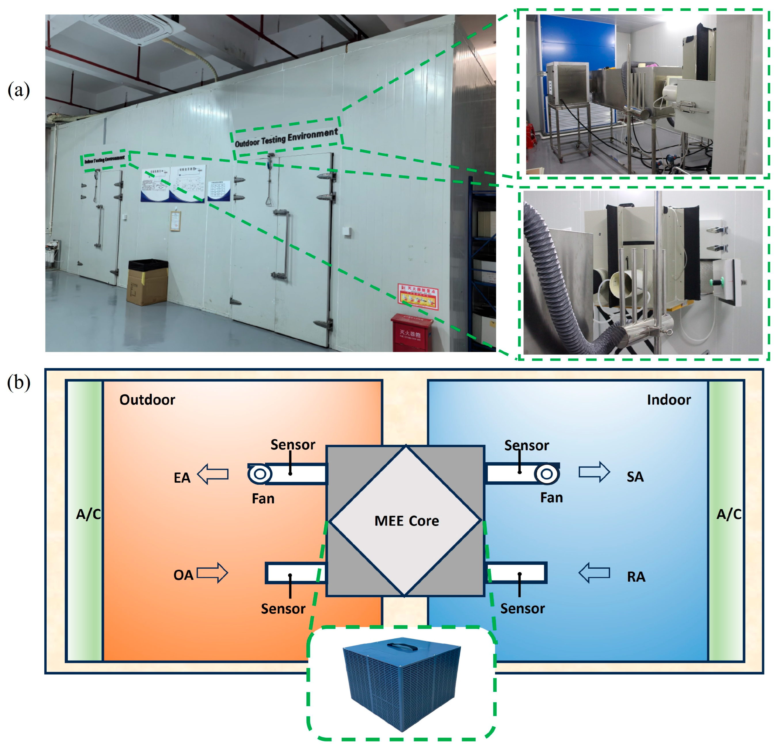
. The experimental system incorporated three calibrated Vaisala HMT333 humidity sensors (accuracy: ±1.0% RH at 25 °C) and T-type thermocouples (accuracy: ±0.5 °C) positioned at both supply/exhaust air streams: (a) humidity validation with saturated salt solutions (LiCl: 11.3% RH, MgCl₂: 33.0% RH, NaCl: 75.3% RH); (b) temperature calibration against a Fluke 724 precision thermometer in water bath (±0.1 °C resolution). Each measurement campaign consisted of five independent replicates under identical operating conditions (ΔT = 15 ± 0.3 °C, φ = 50 ± 2% RH), with data recorded at 10 s intervals over 30 min stabilized periods. Figure 4a presents the enthalpy difference test laboratory for the MEE device, which primarily consists of two refrigeration/heating chambers designed to simulate indoor and outdoor environments. Figure 4b illustrates the layout of the air-to-air total heat exchange ventilator and the test environment utilized to validate the experimental data. The core components of the ventilator include the total heat exchange core, two variable-frequency fans, and multiple temperature and humidity sensors. The fans operate using negative pressure suction to provide airflow, ensuring equal air volume for both the fresh air and exhaust airflow. The tests are conducted in the standard enthalpy difference laboratory in accordance with GB/T 21087-2020. To calculate the sensible heat, latent heat, and enthalpy efficiency of the MEE, the following formulas are employed:

$${\epsilon }_s={\displaystyle \frac{\left(T_{SA}-T_{OA}\right)}{\left(T_{RA}-T_{OA}\right)}}$$

(22)

$${\epsilon }_l={\displaystyle \frac{\left({\omega }_{SA}-{\omega }_{OA}\right)}{\left({\omega }_{RA}-{\omega }_{OA}\right)}}$$

(23)

$${\epsilon }_H={\displaystyle \frac{\left(H_{SA}-H_{OA}\right)}{\left(H_{RA}-H_{OA}\right)}}$$

(24)

Here, T, ω, and H denote temperature (°C), the humidity ratio (kg/kg), and enthalpy (kJ/kg), respectively. The subscripts RA, OA, and SA represent return air, outdoor air, and supply air, respectively.

2.5. Uncertainty Analysis

Measurement uncertainty in the experimental results was evaluated following Moffat’s method [49], using the root-sum-square (RSS) approach. For CFD simulations, numerical uncertainties were quantified via the grid convergence index (GCI < 1.8%) and turbulence model sensitivity tests (±5% eddy viscosity variation). The baseline model exhibited higher uncertainties (±2.1–2.5%) due to simplified assumptions, while the turbulence-enhanced model with vortex generators reduced errors to ±1.5–2.0%. Winter conditions showed marginally higher uncertainties than summer (e.g., ±1.7–2.4% vs. ±1.5–1.8%) due to viscosity effects. Detailed values are shown in

Table 5. Experimental and CFD uncertainties of sensible, latent, and enthalpy efficiencies in summer and winter conditions.

Condition	Parameter	Experimental Uncertainty (±%)	CFD Model Uncertainty (±%)	CFD Model with Turbulent Uncertainty (±%)
Summer	Sensible efficiency	1.2	2.1	1.5
	Latent efficiency	1.6	2.5	1.8
	Enthalpy efficiency	1.4	2.3	1.6
Winter	Sensible efficiency	1.3	2.0	1.7
	Latent efficiency	1.7	2.4	2.0
	Enthalpy efficiency	1.5	2.2	1.8

.

$$U=\sqrt{{\left({\displaystyle \frac{\mathit{\partial }Y}{\mathit{\partial }T}}{U}_T\right)}^2+{\left({\displaystyle \frac{\mathit{\partial }Y}{\mathit{\partial }RH}}{U}_{RH}\right)}^2+{\left({\displaystyle \frac{\mathit{\partial }Y}{\mathit{\partial }V}}{U}_V\right)}^2}$$

(25)

$${ U}_{CFD}=\sqrt{{\left(GCI\right)}^2+{\left(∆Y_{model}\right)}^2}$$

(26)

where $U_T$, $U_{RH}$, and $U_V$ denote the uncertainties associated with temperature, humidity, and airflow velocity measurements, respectively. Sensitivity coefficients ($\mathit{\partial }Y/\mathit{\partial }T$, $\mathit{\partial }Y/\mathit{\partial }RH$, $\mathit{\partial }Y/\mathit{\partial }V$) were calculated based on the experimental correlations obtained from the measured data. Through this uncertainty propagation analysis, the combined uncertainties for the temperature exchange efficiency, latent heat exchange efficiency, and enthalpy exchange efficiency were quantified and are shown in Table 5.

3. Results and Discussion

3.1. Grid Independence Study

To enhance simulation accuracy while optimizing computational resources, mesh independence verification was rigorously performed. The first-layer boundary mesh height was determined via Y⁺ theory (targeting 30 < Y⁺ < 300 [45] for standard wall functions), ensuring compatibility with the hybrid turbulence model. Theoretical calculations and simulation validation were integrated to achieve grid convergence, with detailed steps outlined below:

$$Y^{+}={\displaystyle \frac{u^{*}Y}{\upsilon }}$$

(27)

$$u^{*}=\sqrt{{\displaystyle \frac{{\tau }_w}{\rho }}}$$

(28)

$${\tau }_w=C_f·{\displaystyle \frac{1}{2}}\rho U^2$$

(29)

In the equation, $u^{\mathrm{*}}$ denotes the friction velocity near the wall, $Y$ represents the distance from the first layer of mesh nodes to the wall, υ is the kinematic viscosity of the fluid, ${\tau }_w$ is the wall shear stress, and $C_f$ is the wall friction coefficient. The friction velocity $u^{\mathrm{*}}$ is dimensionless, and the value of $Y$ calculated in this study is 0.1 mm, which is incorporated into the grid division calculation. To comply with the standard wall function requirements (30 < y+ < 300), we iteratively determined Y = 0.1 mm based on the target y + ≈50, which was subsequently validated through mesh sensitivity analysis.

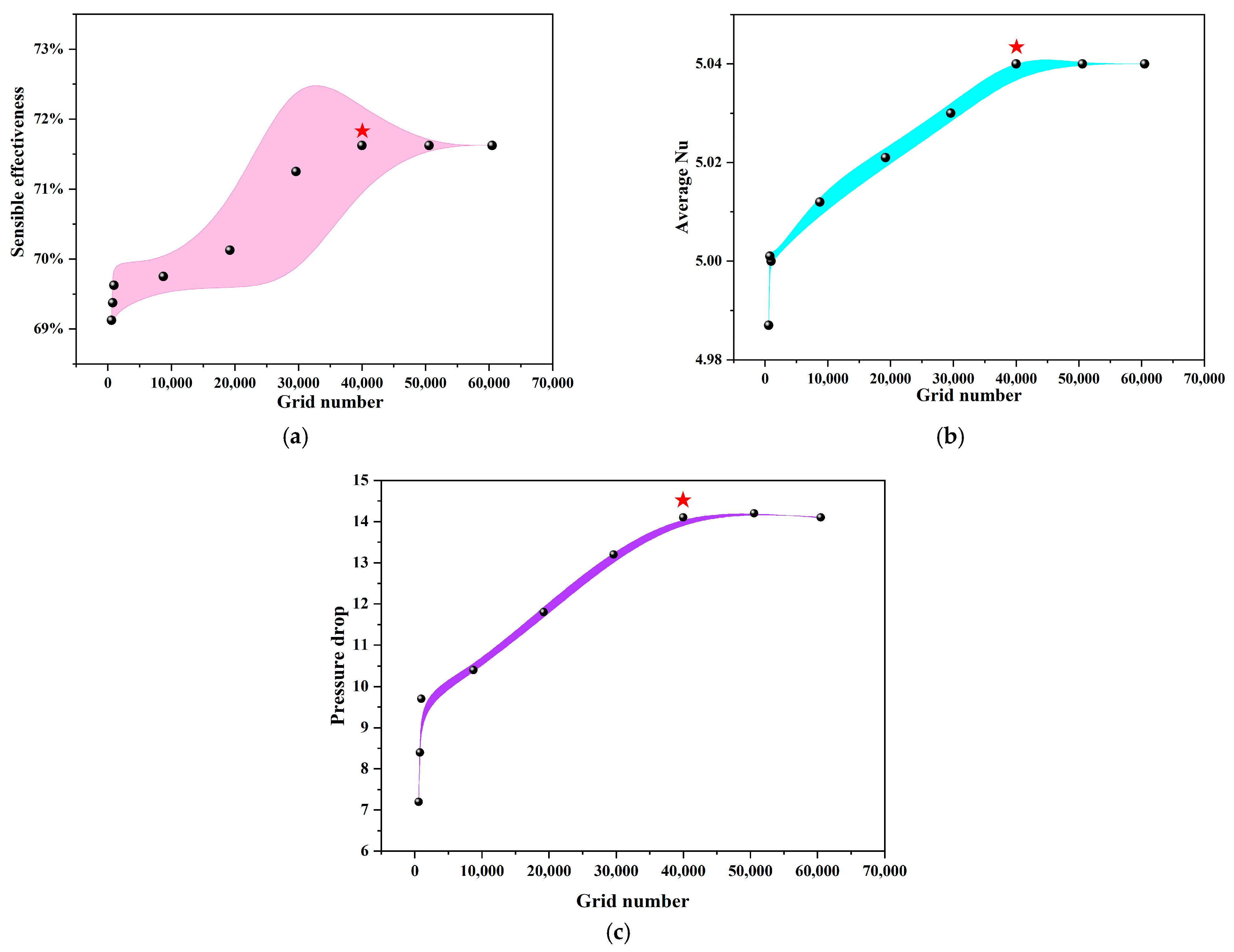
This study conducts nine sets of mesh independence verification on the equivalent model of the test sample at an air velocity of v = 1.1 m/s, evaluating their temperature efficiency ${\epsilon }_s$, Nusselt number (Nu), pressure drop ΔP, and corresponding errors to determine the optimal number of grid cells. As shown in Figure 5, it can be observed that as the number of grids increases, the efficiency value gradually increases until it stabilizes at approximately 71.6%. In all sections of Figure 5, the optimal grid number is marked with an asterisk. The data curve indicates that after optimizing the grid number, the percentage change in effectiveness no longer fluctuates significantly. When the grid count reaches 40,000, the temperature exchange efficiency ${\epsilon }_s$ is 71.63%, the Nu is 5.03, and the pressure drop ΔP is 10.3 Pa. Further increasing the grid size results in negligible changes in temperature exchange efficiency (0.00%), Nu (0%), and pressure drop (0.09%). This indicates that the grid-independent convergence is less than 1.8% and confirms that a grid count of 40,000 is the optimal solution among the nine sets of grid counts.

3.2. Model Optimization

After simplifying the experimental sample into an equivalent model, Figure 6a illustrates the Fluent mesh for the MEE. Figure 6b,c depict the cross-sectional view of the model at x = 133 mm on the y-z plane when the fluid flow velocity is 1.1 m/s, where a laminar flow pattern is evident. This observation confirms the previously mentioned fact that the fluid domain exhibits a fully developed laminar flow. For enhancing single-phase convective heat transfer, this study employs turbulence flow to improve heat and mass transfer [50,51]. Therefore, it is necessary to disrupt the original laminar flow structure and induce turbulence, generating a Kármán vortex street flow, to enhance the heat and mass transfer behavior in the MEE. The standard k-ε turbulence model was selected for its superior accuracy in predicting vortex street shear flows (experimental deviation <1.8%), while grid convergence analysis (GCI < 1.8%) and global sensitivity studies (d = 0.2–0.4 mm) identified the optimal vortex generator diameter as d = 0.3 mm, yielding a Strouhal number (St ≈ 0.21) consistent with classical Kármán vortex theory. According to the theoretical basis for the generation of Kármán vortex streets, when Re < 40, the flow is stable and does not form periodic vortices. When 40 < Re < 30, regular Kármán vortex street formations appear, with vortices alternating in a regular pattern. When 300 < Re < 10,000, the vortex street persists but becomes more complex and irregular in arrangement and shape. Consequently, this study primarily sets up evenly spaced cylindrical disturbance structures at the symmetrical plane of the equivalent model. Based on the experimental test conditions in this study, the required cylinder dimensions to generate Kármán vortex street flow at different flow velocities are calculated, as shown in

Table 6. Cylindrical diameter dimensions that can produce Kármán vortex flow at different air volumes for MEE.

Velocity (m/s)	Re	The Dimensions of the Cylinder Producing the Kármán Vortex Street (mm)
1.10 (150 m3/h)	168	0.69 (27.6%)
1.47 (200 m3/h)	224	0.52 (20.8%)
1.83 (250 m3/h)	280	0.42 (16.8%)
2.20 (300 m3/h)	336	0.35 (13.9%)
2.57 (350 m3/h)	392	0.30 (12%)

. As the fluid velocity increases, the minimum diameter of the Kármán vortex street generator required to produce vortices also increases. However, as the cylinder diameter increases, the pressure difference ΔP in the fluid domain also rises. This creates a trade-off when evaluating the comprehensive performance of the MEE. We need to balance the size of the Kármán vortex street generator. Therefore, we selected a design cylinder diameter of D = 0.3 mm, which increases the resistance interface of the fluid domain by 12%.

For the digital model, the fluid layers consist of two layers, and the mesh is composed of tetrahedral elements. In the Fluent model, the energy equation is enabled. Component transport mode is activated, with component conditions specified in the boundary conditions, and mass transfer is calculated using UDF. The solution method employs the SIMPLE algorithm, with pressure solved using the Second-Order scheme. The momentum equation, H₂O transport equation, and energy equation are solved using the Third-Order MUSCL scheme.

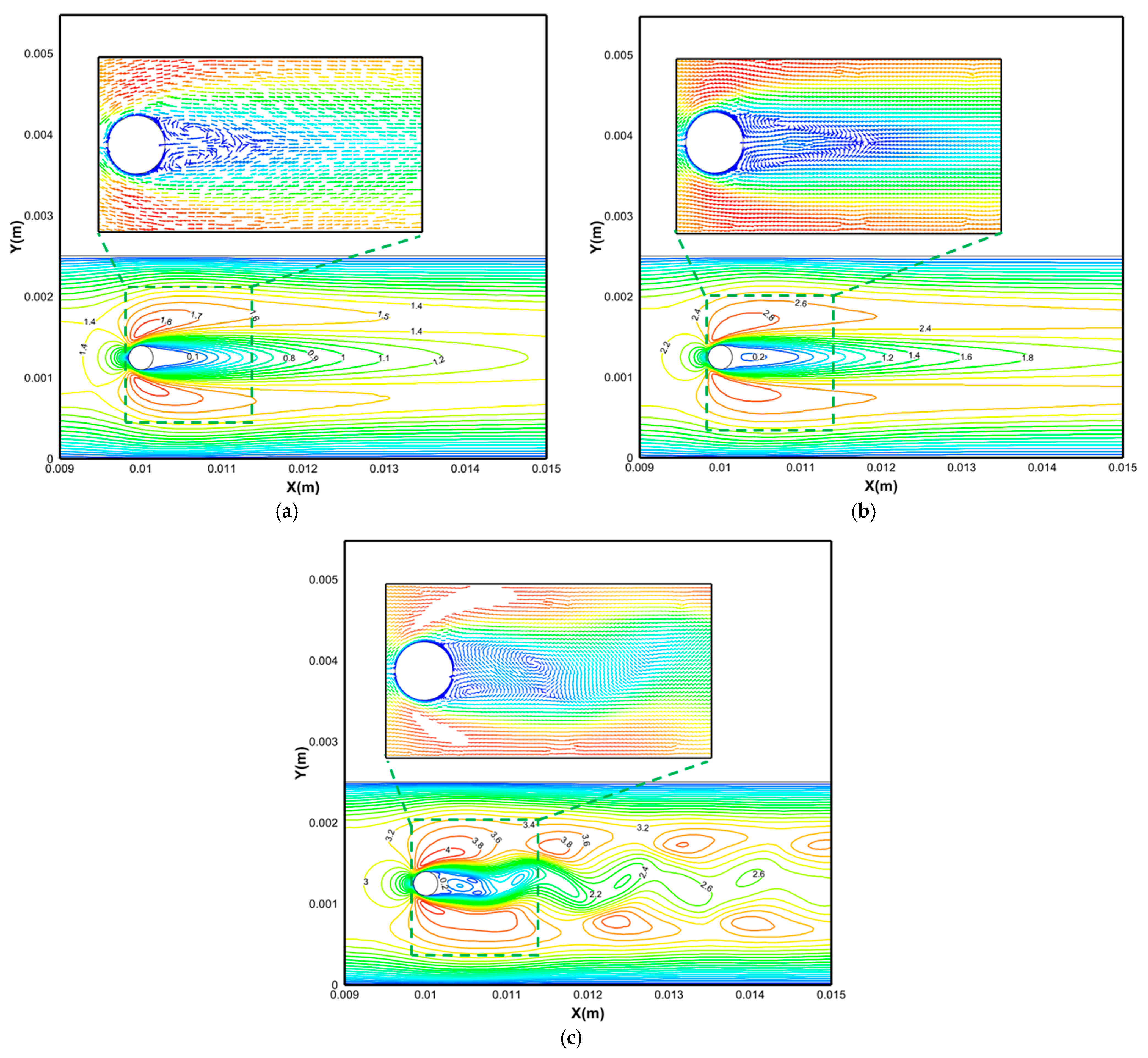
For the optimized model, we primarily calculated the predicted results for the inlet boundary conditions at air velocities of 1.1 m/s, 1.47 m/s, 1.83 m/s, 2.2 m/s, and 2.57 m/s. Representative results with significant changes at air velocities of 1.1 m/s, 1.83 m/s, and 2.57 m/s were selected for the analysis. Figure 7 shows the lift coefficient spectrum of the first Kármán vortex street generator structure at the inlet of the hot fluid domain flow field. Figure 8 presents the flow field contour plot of the first Kármán vortex street generator region in the hot fluid domain. Figure 9 illustrates the local flow field velocity contour plot in the hot fluid domain. When the fluid flow speed is 1.1 m/s, no periodic fluctuation occurs on the cylinder surface. As the iteration steps increase, the lift coefficient remains stable (as shown in Figure 7a), indicating that no Kármán vortex-induced turbulence is formed. The flow field contour plot and velocity cloud plot in the cylinder’s local region also confirm this conclusion. When the fluid flow speed increases to 1.83 m/s, the flow field airflow starts to show fluctuations, but after the flow channel fully develops, it behaves similarly to the situation at 1.1 m/s. In the low-speed flow field with the added cylindrical disturbance structure, no Kármán vortex street-like turbulent structure forms because the Re on the cylinder surface has not reached the critical value required for vortex formation, which requires Re > 40. At flow velocities of 1.1 m/s and 1.83 m/s, the Re on the cylinder surface denotes 20 and 27, respectively. However, it can be observed that as the fluid velocity increases, the velocity gradient rate in the wall membrane area in the contour plot increases. When the fluid flow speed reaches 2.57 m/s, the Reynolds number based on the channel height (2.5 mm) is 392. This places the flow in the subcritical regime (40 < Re < 3 × 10⁵) according to Williamson’s vortex classification [25]. The oscillatory lift coefficient in Figure 7c and periodic vortical structures in Figure 8c and Figure 9c confirm the emergence of an 2S vortex street, characterized by single-row alternating vortices shedding from the cylinder. The Strouhal number (Sr = 0.21) aligns with classical 2S dynamics in this Re range [25], further validating the observed flow patterns.

$$f=S_r\cdot {\displaystyle \frac{\nu }{D}}$$

(30)

When Re < 3 × 10⁵, Sr can be approximated as 0.21. V is the fluid velocity (m/s), and D is the characteristic length of the flow obstruction (m). Therefore, the theoretical vortex shedding period is calculated to be 5.56 × 10⁻⁴ s, which has an error of 3.60% compared to the simulated vortex shedding period of 5.76 × 10⁻⁴ s. This closely matches the actual predicted result. In Figure 8c and Figure 9c, periodic turbulent flow can be observed within the fluid domain. The 2S vortex street generates coherent vortical structures that periodically destabilize the thermal and concentration boundary layers, amplifying momentum and mass transfer through advective mixing, a mechanism critical to the observed heat and mass transfer enhancement. The direction of this turbulent airflow group, when the angle θ between the movement direction of the airflow and the vector direction of the inlet fluid is not 90°, results in a significant velocity gradient near the wall. This indicates that the fluid is being compressed and moves towards the wall, concentrating heat towards the wall and ultimately enhancing the heat and mass transfer processes. Future studies could explore higher Re regimes (e.g., 2P or P + S vortex modes) to assess their potential for further performance optimization [25]. Next, the performance evaluation of the MEE device will be analyzed based on the predicted results.

3.3. Comparison Analysis of Different Model Configurations with Experimental Results

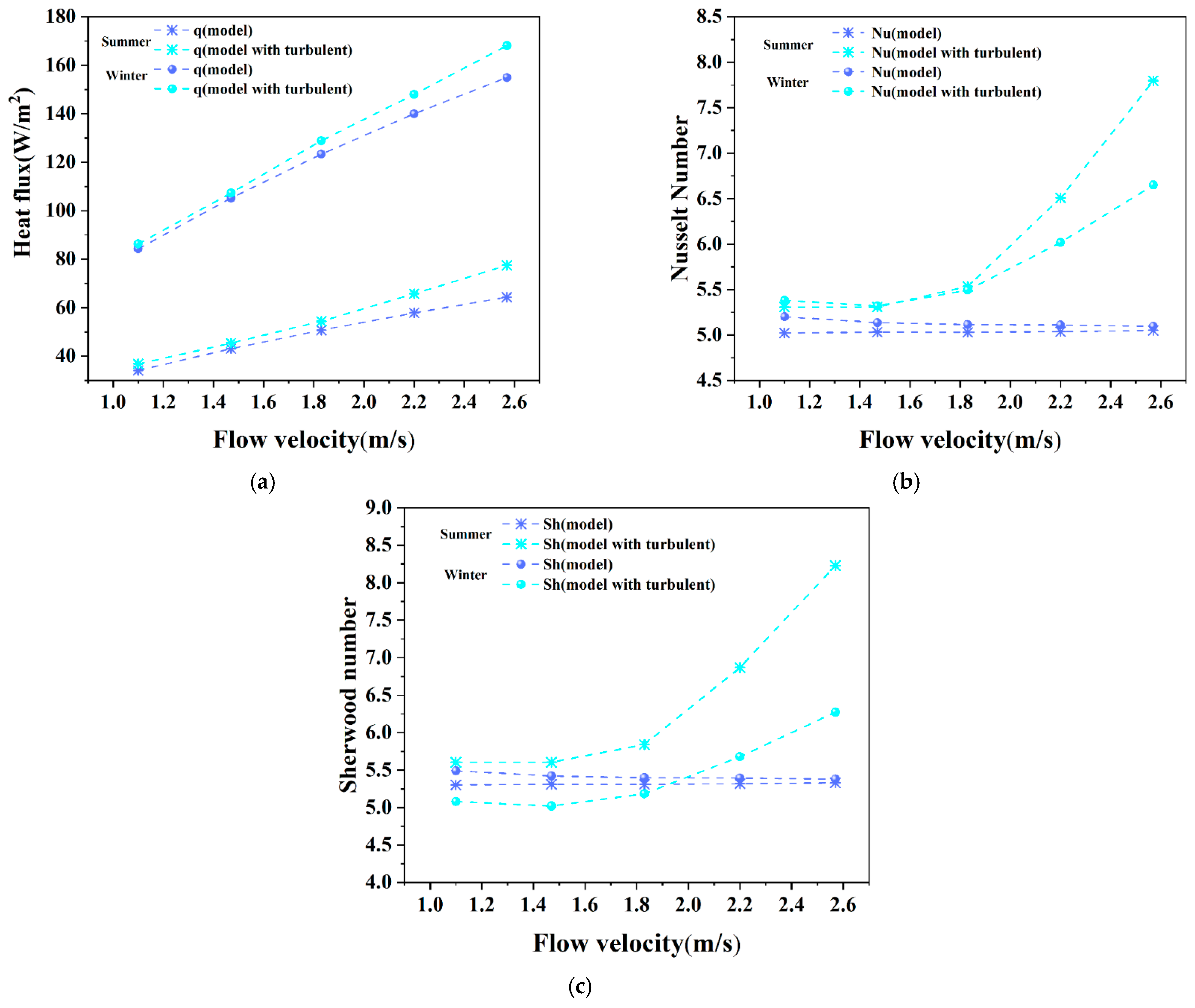
Through the analysis presented above, it is evident that the flow field of the optimized fluid within the model’s fluid domain undergoes a transformation at a specific velocity, resulting in the formation of a Kármán vortex street airflow pattern. Figure 10 illustrates the heat flux, Nu, and Sherwood number (Sh) profiles of the model’s membrane wall under varying fluid flow rates.

As illustrated in Figure 10, both the equivalent and optimized models show that the heat flux of the membrane wall increases with rising fluid flow velocity. However, when the flow velocity reaches 11.83 m/s, a significant increase in the average Nu is observed under both winter and summer conditions, deviating from the previously established linear trend. At a flow velocity of 2.57 m/s, the optimized model exhibits an average Nu of 7.8 and an average Sh of 8.3 in summer, while in winter, these values are 6.7 and 6.3, respectively. Compared to the equivalent model, the flow characteristics improve by 54.35% and 30.49%, respectively. The greater enhancement observed in summer is attributed to two key mechanisms: (1) higher ambient humidity amplifies water vapor diffusion flux ($J=-D\cdot \nabla C$, Fick’s law), significantly boosting latent heat transfer; (2) membrane hygroscopicity under humid conditions increases surface adsorption capacity, temporarily enhancing vapor permeability despite long-term swelling risks. In contrast, winter conditions prioritize sensible heat transfer due to limited vapor concentration gradients, while membrane permeability is optimized to suppress condensation without sacrificing mass transfer efficiency.

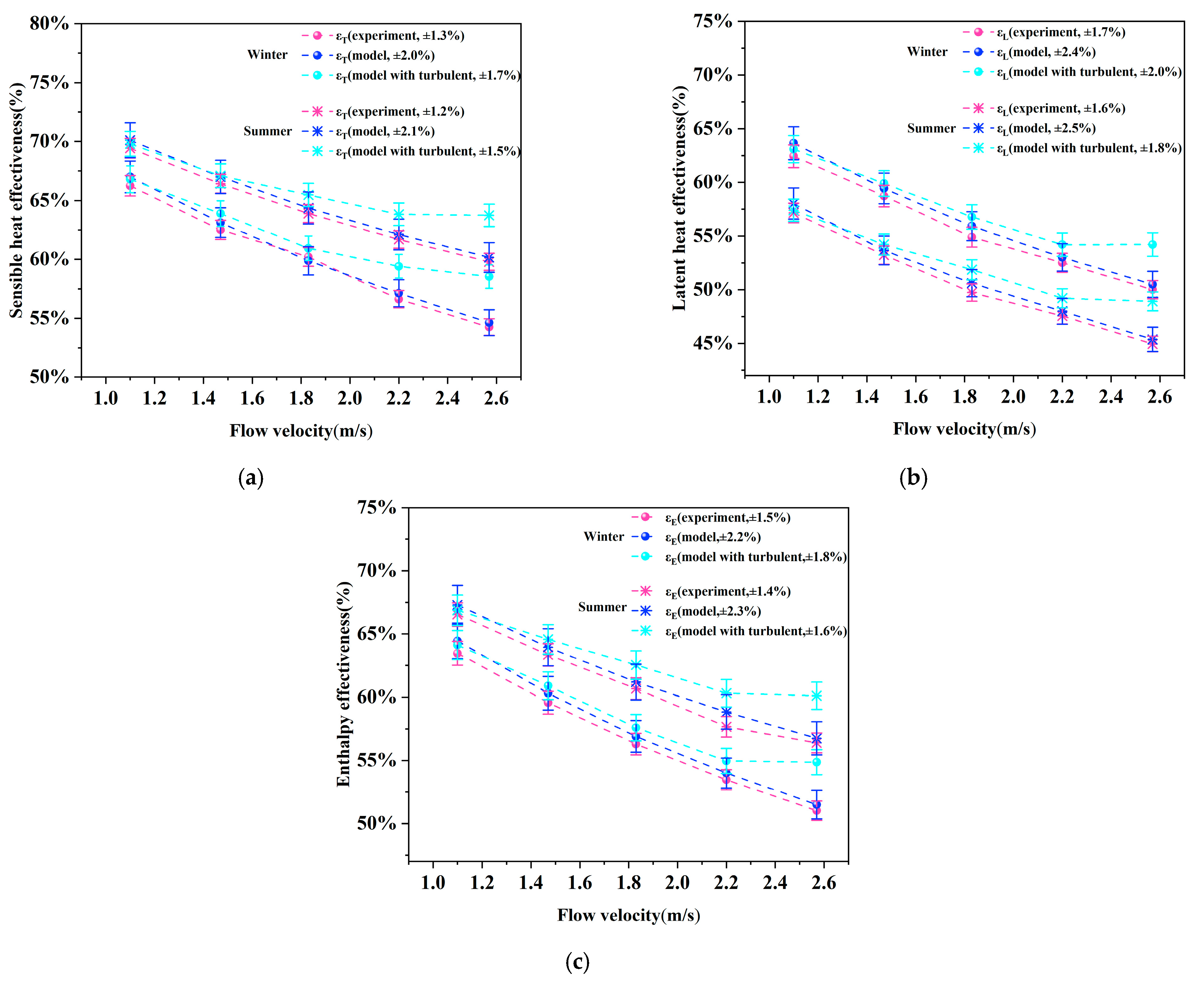
The performance efficiencies of the MEE under winter and summer conditions are systematically compared in Figure 11. The experimental results show strong agreement with the turbulence-enhanced model predictions, with expanded uncertainties of ±1.5–1.8% (summer) and ±1.7–2.0% (winter), as quantified in Table 5. Notably, at low flow velocities (<1.5 m/s), the optimized model (with cylindrical vortex generators) aligns closely with the baseline model (dashed lines) due to the absence of coherent Kármán vortex shedding, resulting in similar heat–mass transfer dynamics. As the flow velocity increases to 2.57 m/s, the turbulence-enhanced model demonstrates a 3.37% (summer) and 3.36 (winter) improvement in enthalpy efficiency compared to the baseline model. This enhancement is attributed to periodic vortex-induced boundary layer renewal, which disrupts the laminar concentration gradient and amplifies latent heat recovery. Seasonal variations further highlight the model’s robustness: winter conditions exhibit marginally higher uncertainties (±2.0%) than summer (±1.8%), consistent with the viscosity-driven flow resistance effects observed in Section 3.2. To address practical HVAC velocity variations, Figure 11 indicates that the enthalpy efficiency gain decreases to 2.1% at 1.83 m/s (Re ≈ 280), where vortex shedding is incomplete. Beyond the tested range, preliminary extrapolation of the efficiency curve suggests a gradual decline in enhancement (e.g., ~3.2% at 3.0 m/s, Re ≈ 450), accompanied by a potential pressure loss increase of ~15%. These observations imply that Re = 392 represents a region of optimal balance between efficiency gains and flow resistance, though further validation is needed for extended operational ranges. It is noteworthy that this study focuses on extreme seasonal conditions (peak summer/winter) to establish baseline performance boundaries for the membrane-based enthalpy exchanger (MEE). However, the theoretical framework—governed by Fickian diffusion dynamics and humidity-dependent membrane hygroscopicity—can be extended to predict transitional seasons (e.g., spring/fall) or other climatic zones by dynamically adjusting vapor concentration gradients (∇C) and permeability coefficients. This adaptability highlights the model’s generalizability and provides a foundational research direction for future studies, such as climate-specific optimization strategies or adaptive membrane designs under varying environmental conditions, ensuring broader applicability beyond the current extreme-case scenarios.

The error bars in Figure 11c explicitly differentiate experimental variability (purple) from numerical uncertainties (gray bands for CFD), ensuring transparent validation of the coupled thermal–hygric transport mechanisms.

3.4. Loss and Comprehensive Performance Evaluation

When a turbulent flow structure is introduced into the channel, both the ΔP and the Cf of the fluid flowing through this region increase. The Cf is defined as follows [52]:

$$C_f={\displaystyle \frac{2∆P\cdot D_h}{\rho \cdot L\cdot {V_{air}}^2}}$$

(31)

Here, ρ, D_h, L, and V_air represent air density (kg/m³), hydraulic diameter, channel length, and air velocity, respectively. The hydraulic diameter D_h is defined as the ratio of the cross-sectional area of the fluid domain to its wetted perimeter, which can be expressed as follows [52]:

$$D_h={\displaystyle \frac{4V_{cyc}}{A_{cyc}}}$$

(32)

where V_cyc denotes the volume of the target fluid domain and A_cyc signifies the effective contact area between the solid domain and the fluid domain. For this study, the hydraulic diameter D_h is 2.5 × 10⁻³ m.

Figure 12 illustrates the curves of ΔP and Cf. The incorporation of the Kármán vortex generator results in a 10% to 40% increase in ΔP and a 29% to 55% increase in Cf. Specifically, at a flow rate of 2.57 m/s (350 m³/h), ΔP increases by 36%, while Cf rises by 41%. Although the addition of a Kármán vortex generator can enhance heat and mass transfer by inducing forced turbulent airflow, it also leads to higher friction coefficients and increased pressure loss. To evaluate the net energy benefit, a simplified energy balance was performed. The electrical power penalty from added pressure loss is calculated as follows:

$$P_{fan}={\displaystyle \frac{∆P\cdot Q}{{\eta }_{fan}}}$$

(33)

$${ P}_{recovered}={\eta }_{recovered}\cdot \rho \cdot Q\cdot c_p\cdot ∆T$$

(34)

For Q = 350 m³/h, η_fan = 60%, and ρ = 1.2 kg/m³, the analysis shows contrasting seasonal outcomes: summer conditions (η_E = 3.37%, ΔT = 8 K) yield a net energy loss of 2.7 W, while winter conditions (η_E = 3.36%, ΔT = 19 K) achieve a net gain of 11.0 W. This divergence highlights that summer’s negative net recovery and winter’s positive net recovery necessitate climate-specific engineering considerations for practical HVAC integration.

Therefore, optimizing the heat and mass transfer performance of MEE devices through structural modifications necessitates a comprehensive evaluation of potential performance trade-offs. This paper will assess the optimization value through an in-depth performance evaluation. To fully evaluate the flow and heat transfer performance of the MEE, the product (fRe) of the drag coefficient Cf and the Re is considered [53]. As shown in Figure 12c, the addition of the Kármán vortex generator increases the fRe value from 32 to 41, with the maximum value of 41 occurring at a Re of 388. This indicates a significant change in the fluid flow characteristics. Future designs could mitigate ΔP penalties through aerodynamic refinements (e.g., streamlined vortex generators) while retaining efficiency gains, a critical step toward practical HVAC integration.

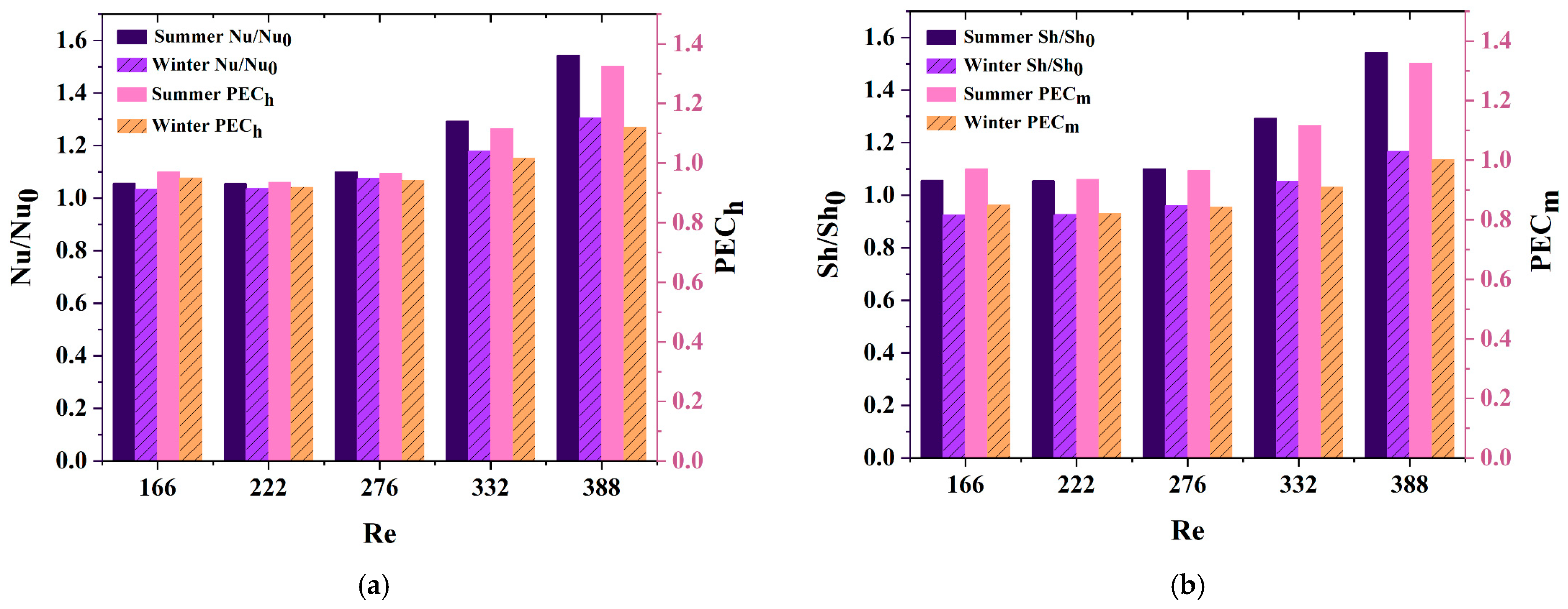
To comprehensively evaluate the flow and heat transfer performance of the MEE, the performance evaluation criterion (PEC) [54] is commonly utilized as follows:

$$PEC={\displaystyle \frac{\frac{Nu}{{Nu}_0}}{{\left(\frac{f}{f_0}\right)}^{\frac{1}{3}}}}$$

(35)

Here, the subscript 0 denotes the initial state as represented by the equivalent model. Nu/Nu0 and Sh/Sh₀ represent the relative Nu and the relative friction factor, respectively. For MEE devices, if the PEC ratio exceeds 1, this indicates that the enhancement in heat transfer performance outweighs the increase in resistance. Conversely, a PEC ratio less than or equal to 1 suggests a disadvantageous trade-off. In this context, PEC_h and PEC_m denote the evaluation indices for heat and mass transfer, respectively.

As illustrated in Figure 13, the ratios Nu/Nu₀ and Sh/Sh₀ initially exhibit a gradual increase, followed by a more pronounced rise after the inflection point at a Re of 276. Notably, the PEC values remain below 1 up to this point, indicating suboptimal overall device performance. However, when a Re reaches 332, both PEC_h and PEC_m exceed 1, signifying a significant enhancement in the device’s overall performance. The optimal performance occurs at a Re of 388, where PEC_h and PEC_m achieve their maximum values of 1.33 and 1.22, respectively. Furthermore, the summer operating conditions demonstrate superior performance compared to the winter conditions, particularly in terms of thermal efficiency, as evidenced by the curves presented in Figure 13a,b.

4. Conclusions

A three-dimensional computational fluid dynamics (CFD) model was established to simulate coupled heat and mass transfer in membrane-based enthalpy exchangers (MEEs). Through theoretical optimization integrating cylindrical vortex generators, periodic Kármán vortex shedding was achieved, enhancing thermal–hygric transport efficiency. Systematic analysis of heat flux, Nusselt number (Nu), Sherwood number (Sh), pressure drop (ΔP), friction coefficient (C_f), and performance evaluation criterion (PEC) yielded the following key findings:

• Model Validation

The CFD results align with experimental data within a 1% discrepancy, confirming the model’s reliability in predicting MEE performance under both steady and vortex-enhanced conditions.

2.

Vortex-Enhanced Efficiency

Cylindrical spoilers induced effective Kármán vortices at 2.57 m/s flow velocity, improving temperature, latent heat, and enthalpy exchange efficiencies by 3.37–3.91% compared to the baseline. Seasonal energy balance revealed a net loss of 2.7 W under summer conditions (ΔT = 8 °C) versus a net gain of 11.0 W in winter (ΔT = 19 °C), necessitating climate-specific deployment strategies.

3.

Energy Penalty Trade-offs

Vortex generation increased ΔP by 36% and C_f by 41% at 2.57 m/s (350 m³/h). While PEC peaked at 1.33 (heat) and 1.22 (mass) when Re = 388, efficiency gains diminished outside the optimal Re range (300–400), constrained by incomplete vortex shedding (Re < 270) and turbulence dissipation (Re > 450).

4.

Practical Implications and Limitations

The winter-biased energy recovery supports prioritized adoption in heating-dominated climates. Scalability to industrial ERV cores may leverage modular multi-cell arrays with geometry ratios L/D = 5–30, though transient sorption hysteresis and manufacturing costs require further analysis. Current limitations include steady-state assumptions and single-row vortex testing; future work will explore multi-row staggered configurations and techno-economic lifecycle assessments.