Article

The Temporal and Spatial Characteristics of Wind–Photovoltaic–Hydro Hybrid Power Output Based on a Cloud Model and Copula Function †

1
School of Water Resources and Hydropower Engineering, North China Electric Power University, Beijing 102206, China
2
Economic and Technological Research Institute, State Grid Qinghai Electric Power Company, Xining 810000, China
*
Author to whom correspondence should be addressed.
This paper is an extended version of our paper published in 2022 6th International Conference on Power and Energy Engineering Conference, Shanghai, China, 25–27 November 2022; pp. 7–11.
Energies 2024, 17(5), 1024; https://doi.org/10.3390/en17051024
Submission received: 22 January 2024 / Revised: 12 February 2024 / Accepted: 16 February 2024 / Published: 22 February 2024
(This article belongs to the Section A: Sustainable Energy)

Abstract

:
In a high proportion of wind–photovoltaic–hydro hybrid power systems, fluctuation and dispersion make it difficult to accurately quantify the output characteristics. Therefore, in this study, a cloud model and copula correlation coefficient matrix were constructed for a hybrid power generation system based on the output data. Multiple backward cloud transformation based on the sampling-with-replacement method was proposed to calculate the improved entropy and hyperentropy to analyze the fluctuation range and dispersion degree quantitatively. A similarity index was proposed to evaluate the similarity between wind power, PV power, and hydropower. A suitable copula function was selected, and the Kendall and Spearman coefficients show the correlation relationships of the hybrid systems. The temporal and spatial characteristics of the hybrid systems were analyzed based on the two models. A typical example in Qinghai proved the effectiveness and applicability of the method. The results show that the correlation between photovoltaic power and hydropower is better and that, in summer, hydropower can be used to adjust the output of renewable energy.

1. Introduction

With the rapid development of renewable energy and the goals of energy policies [1], the impact of high-penetration power systems is becoming increasingly obvious [2]. Wind power and photovoltaic power have strong randomness and volatility [3]. Large-scale integration into the power grid will cause the problem of insufficient system flexibility [4], which, in turn, will cause large-scale power abandonment [5]. Given its large scale [6], good regulation performance [7], and clean, environmentally friendly, and high-quality energy [8], hydropower can effectively stabilize the output fluctuations in wind and photovoltaic power [9]. In the current energy context, wind power, photovoltaic power, and hydropower have gained importance due to their abundant resources and low pollution [10]. Constructing a high proportion of clean-energy power systems is an inevitable trend in the development of global power systems [11].
In order to analyze the temporal and spatial characteristics of the wind–photovoltaic–hydro hybrid power output, researchers have carried out a large amount of research from different perspectives [12]. On the one hand, many researchers only pay attention to the simple mathematical model of hybrid stations [13]. For instance, Zhao et al. quantified and evaluated the degree of power generation complementarity of various energy systems within a certain time scale by defining a complementary coefficient [14]. Chen et al. used the copula function to model and describe the load-matching abilities of multiple renewable energy stations so as to obtain the complementary evaluation of the renewable energy outputs [15]. Tan et al. used the output curve to analyze the complementary characteristics of the wind power–photovoltaic power–hydropower system from the perspective of natural and technical characteristics [16]. These models fail to analyze the inherent correlation characteristics of the complementary system output.
On the other hand, at present, the analysis of output power mostly adopts the method of data mining to establish the mapping relationships between the input variables and output of each power generation system [17]. When extreme conditions occur, this deterministic model cannot accurately reflect the overall output of the system [18]. Due to the randomness and fuzziness of renewable energy output, the output curve cannot strictly reflect the change in output [19], and the actual output value should change within a certain range. The cloud model is an algorithm that combines randomness and fuzziness [20]. It is a cognitive model based on the theory of the probability measure space [21]. The model realizes the problems of bidirectional transformation between the qualitative perspective and quantitative perspective [22]. Therefore, it is of great significance to establish a cloud model to describe the output of multi-energy complementary generation systems [23]. Nowadays, there are few studies that build correlation relationships with cloud models. Wang et al. used the cloud model to analyze the correlation between the indicators and warnings of the transmission line operation status [24]. However, single-cloud models fail to construct high-dimensional models. Copulas are widely used to construct multivariate probabilities [25]. Due to the systematic theories, copulas have advantages in correlations between multiple variables [26]. The copula function is often used to measure the correlations of hybrid complementary systems [27]. Because cloud models can only capture the two-dimensional similarity, three-dimensional copulas are constructed to analyze the correlations of wind power–photovoltaic power–hydropower hybrid systems. In addition, the copula function can be used to effectively construct the mathematical relationship between wind power, photovoltaic power, and hydropower. Therefore, the copula function can not only build the correlation coefficient but also improve the computation efficiency. Lin et al. proposed the multivariate Gaussian kernel copula to describe the correlation of wind speeds among multiple wind farms [28]. It is difficult to obtain the exact correlation under different operating conditions with a single copula function.
Based on the idea of the cloud model and copula function, this paper establishes a correlation model to analyze the temporal and spatial characteristics of the wind–photovoltaic–hydro hybrid power output based on the cloud model and copula function.

2. Research Methodology

2.1. Basic Output Cloud

The cloud model combines the randomness and fuzziness of events through three characteristic indexes (expectation E x , entropy E n , and hyperentropy H e ) to form the transformation and mapping between qualitative analysis and quantitative analysis [29]. In this section, the basic structure of cloud theory is given, along with a description of the uncertainty in hybrid systems.
U is a common set of variables x .The set can be described as U = x , and U is a quantitative domain called the domain of discourse. Assume that C is a random qualitative concept on the quantitative domain U . If the quantitative data set x U is a random realization of the qualitative concept μ ( x ) 0 , 1 , and the uncertainty μ ( x ) from x to C is a random number with a stable distribution trend, then the relationship can be expressed by the following relation:
μ ( x ) : U 0 , 1 x U
The distribution of x on the domain U then becomes a cloud model. The quantitative value x is called a cloud droplet, which is used to represent the randomness of the quantitative concept. μ ( x ) is used to represent the degree to which the quantitative concept x belongs to the qualitative concept C ,and it is called the affiliation function.
The cloud model can not only use the affiliation function μ ( x ) to describe the fuzziness of the concept, but also describe the randomness of the affiliation function μ ( x ) and the randomness of the cloud droplets. The range of the affiliation degree is from 0 to 1, and the mapping from x to U is one-to-many, indicating that the affiliation degree is a probability distribution rather than a fixed value, resulting in an ambiguous boundary of cloud, which is not a clear curve. A cloud image is composed of multiple cloud droplets, and each cloud droplet reflects the transformation between quantitative data and qualitative data. It is meaningless to analyze the affiliation degree of a certain point separately, and the entirety of each cloud model can reflect the characteristics of qualitative concepts. When the affiliation function satisfies the following formula, the distribution of random variables composed of all cloud droplets is called the normal cloud model. The normal cloud model is the most common cloud model.
μ ( x ) = exp x E x 2 2 y 2
The cloud generator is a function that establishes the relationship between qualitative and quantitative data, including forward generators, reverse generators, and index approximation methods. This paper uses a reverse generator to estimate the parameters. The statistical method is used to estimate the parameters of the data samples to obtain the digital characteristic parameters of the connotation. In the process of reverse cloud transformation there will inevitably be errors. Excessive prediction faults will make it difficult to achieve two-way transformation between qualitative and quantitative data. The traditional reverse cloud algorithm based on the first-order absolute central moment and the reverse cloud algorithm based on the fourth-order absolute central moment cannot guarantee the following equality. The two algorithms will cause major errors.
S 2 E n 2 > 0
S 2 = 1 N 1 i = 1 N ( x i X ¯ ) 2
X ¯ = 1 N i = 1 N x i
E n = 9 ( S 2 ) 2 μ 4 6 4
μ 4 = 1 N 1 i = 1 N ( x i X ¯ ) 4
where S 2 is the sample variance, N is the number of samples, x i is the sample variable, X ¯ is the average value of the samples, and μ 4 is the fourth-order central moment.
The reverse cloud algorithm based on the first- and fourth-order absolute central moments directly obtains the digital characteristic parameters of the cloud model through the moment estimation of different orders, that is, the single-step estimation, ignoring the characteristics of the cloud droplets being generated by two random processes.
Multiple backward cloud transformation based on sampling replacement (MBCT-SR) was used in this study. MBCT-SR is a multi-step cloud transformation process [30], and through random sampling grouping, E x and H e are generated in different subset intervals, which increases the stability [31]. The algorithm for calculating hyperentropy and cloud entropy used in this work can ensure that the estimation of hyperentropy will not appear as an imaginary number and has strong stability [32].
The expectation E x is the central value of the cloud droplets in the domain space, that is, the average output of the wind–photovoltaic–hydropower complementary power generation system.
E x = X ¯ = 1 N i = 1 n x i
The entropy E n is the value range of cloud droplets in the domain space, which reflects the uncertainty information in the cloud model and represents the fluctuation range of output in the complementary system.
Y i 2 = 1 n 1 j = 1 n ( x i j x ¯ i ) 2
E n 2 = 1 2 4 ( E Y 2 ) 2 2 Y 2
where Y i 2 is the variance of random samples by MBCT-SR, n is the number of elements contained in each random sample by MBCT-SR, and x i j is the random samples of MBCT-SR.
The hyper entropy H e is the uncertainty of the cloud entropy in the domain space, reflecting the randomness of the dispersion and membership degrees of the cloud droplets, and it also describes the concentration degree of the output in the fluctuation range in the complementary system. The greater the hyperentropy, the greater the degree of dispersion of the cloud, the greater the randomness of the membership degree, and the greater the thickness of the cloud.
H e 2 = E Y 2 E n 2
Through the above process, a certain input sample is transformed into three eigenvalue forms of the cloud model, and the output quantitative distribution characteristics in each input variable interval are obtained.
An example is displayed for clarity. A cloud model with the parameters E x = 4 , E n = 1 , and H e = 0.1 is shown in Figure 1. The cloud model uses the distribution of cloud drops to reflect the robustness and fuzziness of the qualitative concept.

2.2. Output Cloud Similarity

Cloud models can not only provide uncertainty representation in data mining but also provide qualitative analysis methods; this is more in line with human cognition for mining results. In general, quantitative data can be transformed into qualitative data through a cloud model, and data mining tasks based on qualitative concepts require similarity measurements.
According to the output cloud model of wind power, photovoltaic power, and hydropower, the similarity between two output clouds is calculated to reflect and evaluate the degree of correlation between each power generation system, which provides a basis for extracting the complementarity and differences of the wind–photovoltaic, wind–hydropower, and hydropower–photovoltaic power generation systems.
Assuming that the Euclidean distance between the output cloud a and output cloud b is d a , b , the calculation formula is as follows [33].
d a , b = 1000 / ( E x a E x b ) 2 + ( E n a E n b ) 2 + ( H x a H x b ) 2

2.3. Correlation Degree Based on the Copula Function

The copula can reflect the multivariate joint probability distribution with marginal distribution [34]. Compared with other simple correlation models, such as the regression model, the copula function can better capture the tail relationship. Therefore, copula functions are generally used to build correlation models for hybrid systems [35]. The copula density can be expressed as
U ( x 1 , x 2 , , x a ) = C ( F 1 ( x 1 ) , F 2 ( x 2 ) , F n ( x a ) )
where U ( x a ) is the joint distribution of variables x a , and F a is the marginal distribution of x a .
If F x is a continuous function, the joint probability function can be calculated with (12).
u ( x 1 , x 2 , , x a ) = C ( F 1 ( x 1 ) , F 2 ( x 2 ) , F a ( x a ) ) i = 1 a f a ( x a )
where f ( x a ) is the marginal density function.
The Kendall coefficient and Spearman rank correlation coefficient were selected as the correlation coefficient methods. The two evaluation indicators were calculated based on a suitable copula function [36].
The Kendall coefficient ρ τ is calculated as
ρ τ = P A 1 A 2 B 1 B 2 > 0 P A 1 A 2 B 1 B 2 < 0
where P · is the probability operation. A i and B i are independent variables.
The Spearman rank correlation coefficient ρ s is calculated as
ρ s = 3 P A 1 A 2 B 1 B 3 > 0 A 1 A 2 B 1 B 3 < 0
The copula functions are divided into the elliptic family and the Archimedes family. The elliptic copula contains a Gaussian copula and a t-copula. Compared with the Archimedes copula family, the elliptic family copula can show high-dimensional correlation characteristics. Therefore, this paper selects the Gaussian copula and t-copula to construct the three-dimensional copula function.
The probability distribution function of the Gaussian copula is expressed as
C u 1 , u 2 , u 3 = Φ Φ 1 u 1 , Φ 1 u 2 , Φ 1 u 3
where Φ 1 is the inverse function of the standard normal distribution function.
The probability distribution function of the t-copula is expressed as
C u 1 , u 2 , u 3 ; ρ , v = T v ( T v 1 ( u 1 ) , T v 1 ( u 2 ) , T v 1 ( u 3 ) )
T v 1 is the inverse function of the unary t distribution function, the degree of freedom of which is v .
The root mean square error ( R M S E ), Akaike information criterion ( A I C ), and Bayesian information criterion ( B I C ) were selected to judge the fitness of the model.
R M S E = i = 1 n ( E p i E i ) 2
A I C = N log ( i = 1 n ( E p i E i ) 2 ) + 2 k
B I C = k ln ( N ) + N log ( i = 1 n ( E p i E i ) 2 )
where E p i is the predicted value of the copula function, E i is the real value of the copula function, and k is the number of copula function parameters.

3. Results and Discussion

3.1. Basic Data

This paper takes a wind–photovoltaic–hydropower complementary power generation system in Qinghai, China as an example for analysis. Qinghai Province is located in the northeast of China, and the quantity of wind, photovoltaic, and hydropower is abundant [37]. The rich energy storage volume and vast Gobi desert conditions are appropriate for the development of a hybrid system [38]. The wind–photovoltaic–hydropower hybrid system in the study area was a typical complementary structure, and it clearly reflects the power cases. The actual data of the power generation system from 00:00 on 13 November 2022 to 23:00 on 13 November 2023 were selected to form the data sample library, and the sampling interval was 1 h. The output of the hybrid system in the typical year is shown in Figure 2. In this multi-energy complementary system, due to the proximity to the Yellow River, hydropower resources are abundant, and hydropower output is much larger than wind power and photovoltaic output. In addition, the installed capacity of photovoltaics in this area is small, and the wind power output is greater than the photoelectric output. The wind and photovoltaic output experienced great uncertainty and variability during the analysis. The power distribution of wind is more disperse compared to the photovoltaic output. Compared with renewable energy, the output of hydropower is steadier.
Violin plots are used to show the distribution and probability density of multiple sets of continuous data. The size of the box depends on the quartile distance and black area of the data. The large box indicates that the data distribution is discrete and fluctuates greatly, while the small box indicates that the data are concentrated. The distribution of the violin plot in Figure 3 shows that the wind power output is larger in April, May, July, and August, and the degree of dispersion is also larger. The output in September, October, November, and December is more concentrated. The output of photovoltaic power is the largest in July, and the output is significantly larger than that of the other months. The output of photovoltaic power is larger in spring and summer, and the output is more concentrated in autumn and winter. The hydropower output is larger and more concentrated in July and August, and the output is the most dispersed in December. The output is larger in summer and smaller in winter.
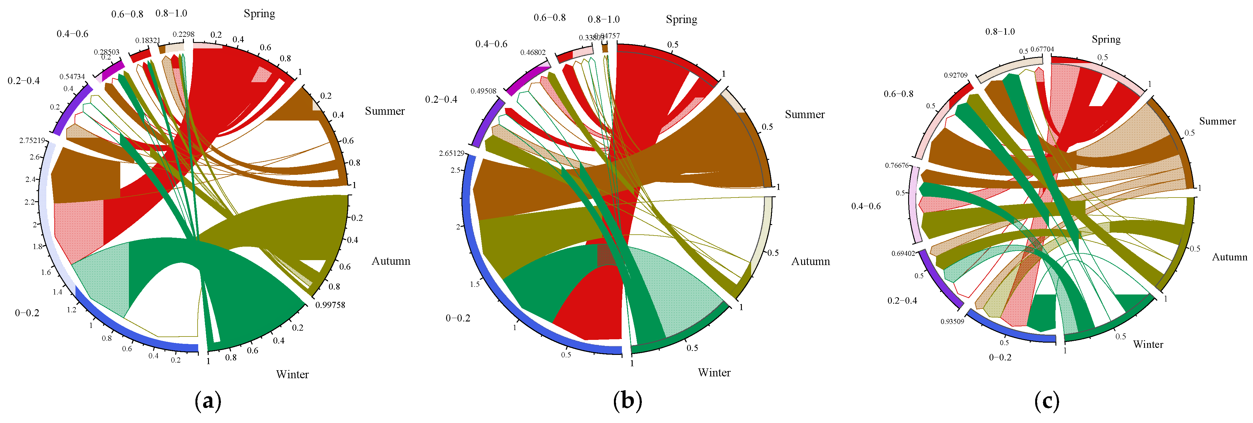
The distribution of the complementary system in each output interval was analyzed using the string diagram in Figure 4, and the normalized output was divided into five intervals: lowest, lower, medium, higher, and highest output intervals. The wind power output was concentrated in the [0,0.2] output interval, and the cumulative normalized output reached 2.75. The output probability interval in summer was larger, and the output probability interval in autumn was smaller. The photovoltaic output was also concentrated in the [0,0.2] interval, and the cumulative normalized output reached 2.65. For the photovoltaic output, the probability interval of [0.8–1] was the smallest, and the photovoltaic output was largest in summer. The distribution of hydropower output in each interval is relatively uniform, and the probability was larger in the output interval of [0.6–0.8] and greater in summer.

3.2. Output Cloud Model Analysis

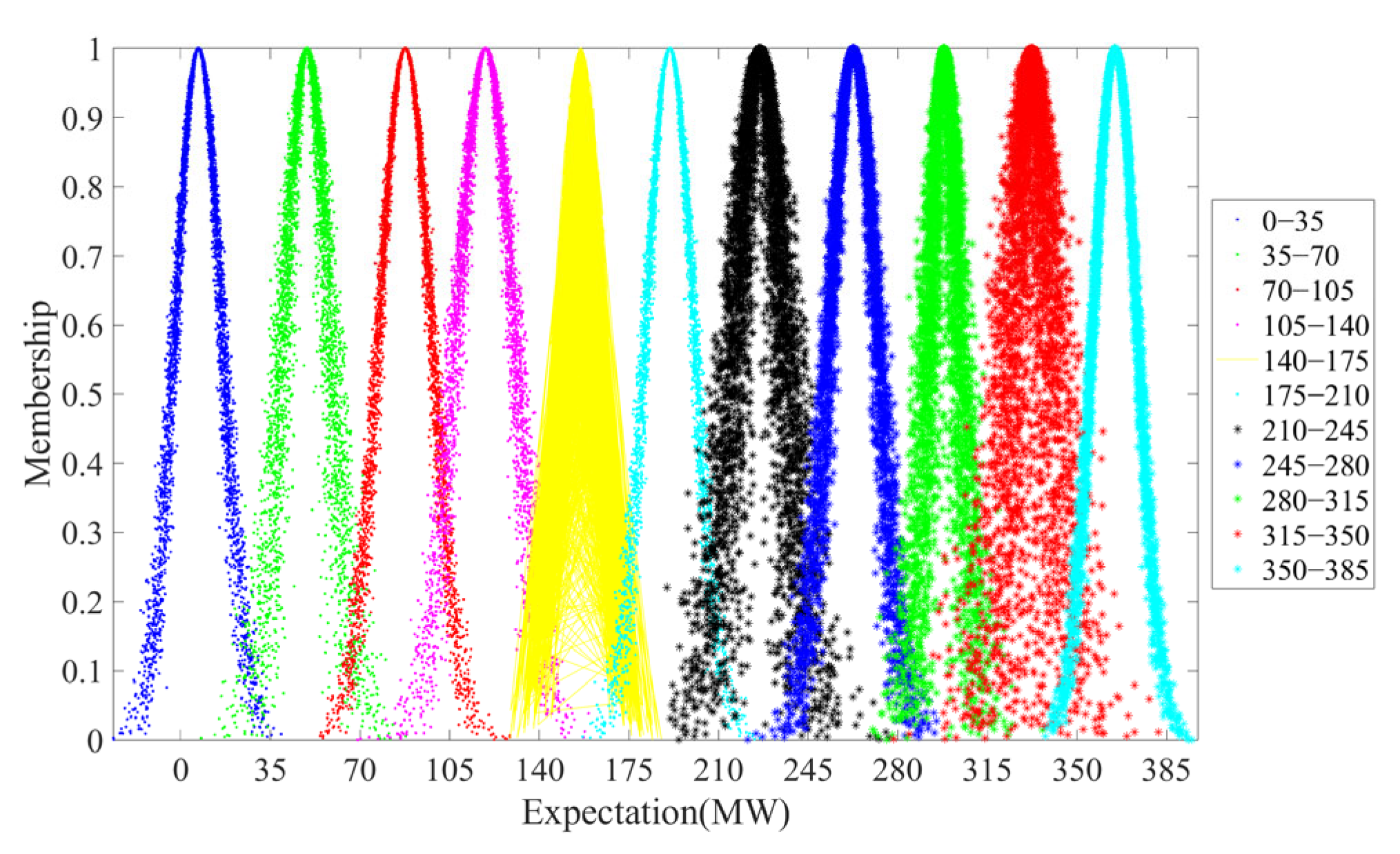
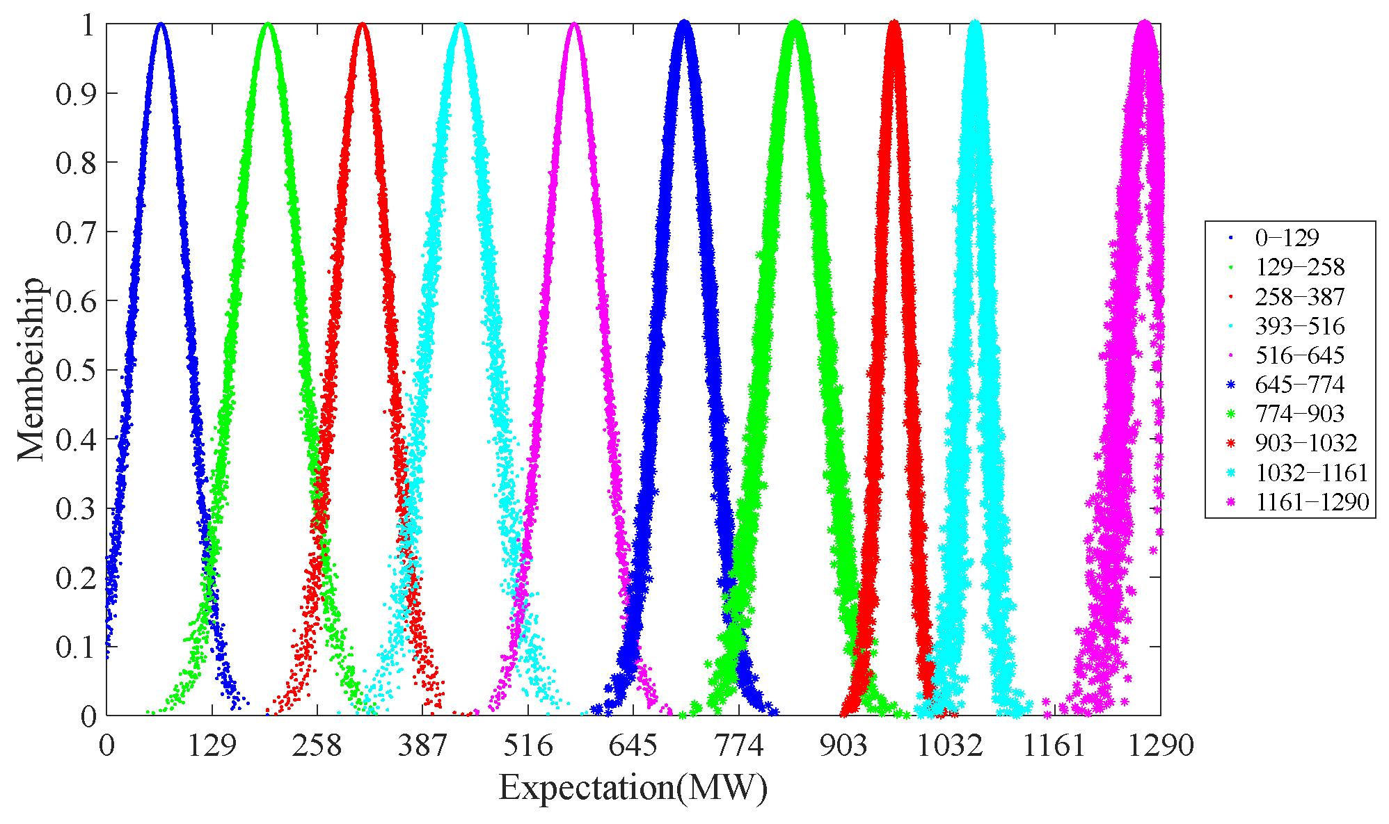
The wind power output, photovoltaic output, and hydropower output were divided into intervals of 35 MW wind power output, 17 MW photovoltaic output, and 129 MW hydropower output, and the outputs of different input variable intervals were counted. The results are shown in Figure 5, Figure 6 and Figure 7.
By constructing the output cloud model of three power sources, the output distribution, fluctuation, and concentration can be seen. In the wind power output distribution between 0 and 385 MW, the entropy in the [105,140] output interval is 11.1638, indicating that the output fluctuation in this interval is large. The entropy in the [280,315] output interval is 5.8725, and the output varies smoothly. The hyperentropy in the [315,350] output interval is 4.735, indicating that the output dispersion in this interval is greater. The hyperentropy in the [350,385] output interval is 0.6644, and the output concentrates in this interval. Overall, the hyperentropy of wind power in each output interval is larger, the dispersion degree of fluctuation is larger, and it has strong uncertainty.
The photovoltaic output is distributed between 0 and 170 MW, with the lowest expected output. The fluctuation range of the output in each output interval does not differ by much. The entropy in the [153–170] interval is 5.4985, and this is the maximum of the photovoltaic power entropy. The output dispersion in the [153,170] interval is large. The output fluctuation of photovoltaic output in each interval is relatively average, and the overall photovoltaic output is relatively stable.
The hydropower output is distributed between 0 and 1290 MW. The entropy in the [1032,1161] output interval is only 14.7385, and the fluctuation degree is the smallest. The entropy of hydropower is the greatest for the hybrid system, indicating that the fluctuation in hydropower is much larger than wind and photovoltaic power in the output interval. The hyperentropy in the [903,1032] output interval is 1.8326, and the output is the most concentrated.
Compared with the output scatter diagram, which can only qualitatively reflect the output trend and fluctuation of the power generation system, the output cloud model quantitatively reflects the output characteristics of each power generation system from qualitative evaluation to quantitative evaluation. It also more intuitively and comprehensively reflects the fluctuation and dispersion degree of each power generation system.

3.3. Cloud Model Similarity

According to the calculation method of cloud similarity, the monthly average outputs of wind power, photovoltaic power, and hydropower were used to calculate the cloud similarity of wind power–photovoltaic power, wind power–hydropower, and photovoltaic power–hydropower generation systems in each month. The results are shown in Table 1.
The wind–photovoltaic complementary system has the highest similarity in January, reaching 29.995, and the highest complementarity in July, with a similarity of 11.891. The wind–hydropower complementary system has the highest similarity in April, reaching 2.439, and the highest complementarity in August, with a similarity of 1.269. The photovoltaic–hydropower complementary system has the highest similarity in April, reaching 2.111, and the highest complementarity in August, with a similarity of 1.160. It can be seen from the above table that the similarity between wind power and photovoltaic power is the highest of the three hybrid systems. In summer, the difference between wind and photovoltaic power output is larger. The similarity between wind power and hydropower, photovoltaic power, and hydropower is the highest in spring, and the difference in summer is the largest. In the summer, hydropower can effectively adjust the wind and photovoltaic power output. The output similarity cloud reflects the difference and complementarity between the output clouds.

3.4. Correlation Analysis of Hybrid Systems

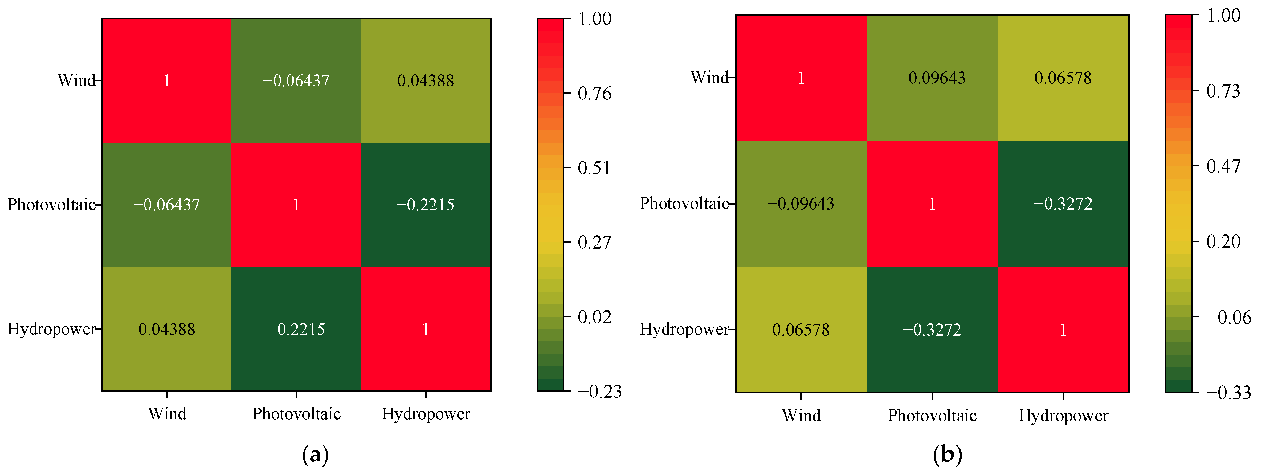
Furthermore, to analyze the correlation of the hybrid systems, the Kendall correlation coefficient and Spearman rank coefficient were used in this study to judge the three-dimensional correlation coefficient. The goodness-of-fit test results are shown in Table 2. The RMSE, AIC, and BIC of the Gaussian copula are all smaller than the t-copula. Therefore, the Gaussian copula was selected to fit the model.
Through the comparison of the two correlation coefficients in Figure 8, it was found that the correlation between photoelectricity and hydropower is the largest, with the Kendall correlation coefficient and Spearman rank coefficient being −0.2215 and −0.3272, respectively. This indicates that hydropower has a high correlation with photoelectricity. The period of large hydropower output is generally when the summer rainfall is large, and at this time, the photovoltaic panel can rarely receive sunlight and generate electricity; therefore, there is a significant negative correlation between the two. The correlation between wind power and hydropower is the smallest, with the Kendall correlation coefficient and Spearman rank coefficient being 0.04388 and 0.06578, respectively. The two correlation coefficients between wind and hydropower are positive, indicating that hydropower and wind power have similar output distributions. Based on the real-world scenario of Qinghai Province, hydropower plays an important role in regulating the output of renewable energy in the complementary system. The correlation coefficient between wind power and photovoltaic power is involved in the correlation coefficient between the other two systems, indicating that there is a certain negative correlation between wind power and photovoltaic power. In the period of large wind power output, photovoltaic output is often small, and this complementary relationship can be used to adjust the daily output of the system.

4. Conclusions

In the current energy context, future power systems are trending toward the construction of a high proportion of wind–photovoltaic–hydro complementary systems. Due to the fluctuation and dispersion of wind power, PV power, and hydropower, it is difficult to accurately quantify the output characteristics of the power generation system. Therefore, a cloud model was constructed in this study to characterize the volatility and dispersion of the complementary system. The MBCT-SR method was proposed to calculate the improved entropy and hyperentropy to quantitatively analyze the fluctuation range and dispersion degree. The similarity index of the output cloud and Kendall and Spearman coefficients of the Gaussian copula was proposed to evaluate the temporal and spatial characteristics of wind–photovoltaic–hydropower hybrid power output.
(1)
The cloud model can be extended from qualitative to quantitative evaluation, which can more accurately reflect the output characteristics. Correlation analysis can characterize the similarity of complementary power generation systems.
(2)
The hyperentropy of the hydropower system is larger than others, meaning the output of hydropower is more concentrated in the interval between 1161 and 1290, and thus the degree of dispersion in the output interval is greater. The wind and photovoltaic outputs have better similarity in January; the index of similarity is 29.995.
(3)
Due to the RMSE, AIC, and BIC, the Gaussian copula is more suitable for describing hybrid systems. The Kendall correlation and Spearman rank correlations of the Gaussian copula were −0.2215 and −0.3272, respectively. The results suggest that the correlation between hydropower and photovoltaic power is better.
In practical applications, the cloud model for hybrid power generation systems can provide a demand reference for peak regulation. The similarity index of the cloud model and Gaussian copula function will promote analysis of the interaction of each subsystem in the hybrid power system.

Author Contributions

Conceptualization, H.M. and F.X.; methodology, H.M. and P.H.; software, C.L.; investigation, C.L. and L.Y.; resources, L.Y.; writing—original draft preparation, H.M. and P.H.; writing—review and editing, H.M. and F.X.; supervision, F.X. All authors have read and agreed to the published version of the manuscript.

Funding

The work was supported by the Science and Technology project of Qinghai Province (2023-GX-158).

Data Availability Statement

The data are available in this paper.

Acknowledgments

The authors thank the reviewers whose comments improved the quality of this paper.

Conflicts of Interest

Authors Chunlai Li and Libin Yang were employed by the State Grid Qinghai Electric Power Company. The remaining authors declare that the research was conducted in the absence of any commercial or financial relationships that could be construed as a potential conflict of interest.

Nomenclature

MBCT-SRMultiple backward cloud transformation based on sampling with replacement Y 2 Variance of random samples by MBCT-SR
RMSERoot mean square error d Euclidean distance between the output clouds
AICAkaike information criterion U ( · ) Joint distribution of variables
BICBayesian information criterion F a Marginal distribution of variables
Parameters u ( · ) Joint probability function of variables
E x Expectation value f a Marginal density function.
E n Entropy C Set of marginal distribution function
H e Hyperentropy ρ τ Kendall coefficient
U Domain of discourse ρ s Spearman rank correlation coefficient
C Random qualitative concept A B Independent random vectors
μ ( x ) Affiliation function Φ 1 Inverse function of the standard normal distribution function
S 2 Variance of samples T v 1 Inverse function of the unary t distribution function
N Number of samples v Degree of freedom
x i Sample variable E p i Predicted value of copula function
X ¯ Average value of samples E i Real value of copula function
μ 4 Fourth-order central moment k Number of copula function parameters

References

  1. Shayan, M.E.; Najafi, G.; Ghobadian, B.; Gorjian, S.; Mazlan, M.; Samami, M.; Shabanzadeh, A. Flexible Photovoltaic System on Non-Conventional Surfaces: A Techno-Economic Analysis. Sustainability 2022, 14, 3566. [Google Scholar] [CrossRef]
  2. Zhu, F.; Zhong, P.; Xu, B.; Liu, W.; Wang, W.; Sun, Y.; Chen, J.; Li, J. Short-Term Stochastic Optimization of a Hydro-Wind-Photovoltaic Hybrid System under Multiple Uncertainties. Energy Convers. Manag. 2020, 214, 112902. [Google Scholar] [CrossRef]
  3. Huang, K.; Liu, P.; Ming, B.; Kim, J.S.; Gong, Y. Economic Operation of a Wind-Solar-Hydro Complementary System Considering Risks of Output Shortage, Power Curtailment and Spilled Water. Appl. Energy 2021, 290, 116805. [Google Scholar] [CrossRef]
  4. Chen, Y.; Wang, Y.; Kirschen, D.; Zhang, B. Model-Free Renewable Scenario Generation Using Generative Adversarial Networks. IEEE Trans. Power Syst. 2018, 33, 3265–3275. [Google Scholar] [CrossRef]
  5. Zhang, Y.; Lian, J.; Ma, C.; Yang, Y.; Pang, X.; Wang, L. Optimal Sizing of the Grid-Connected Hybrid System Integrating Hydropower, Photovoltaic, and Wind Considering Cascade Reservoir Connection and Photovoltaic-Wind Complementarity. J. Clean. Prod. 2020, 274, 123100. [Google Scholar] [CrossRef]
  6. Shayan, M.E.; Najafi, G.; Ghobadian, B.; Gorjian, S.; Mazlan, M. A Novel Approach of Synchronization of the Sustainable Grid with an Intelligent Local Hybrid Renewable Energy Control. Int. J. Energy Environ. Eng. 2023, 14, 35–46. [Google Scholar] [CrossRef]
  7. AN, Y.; Zhao, Z.; Wang, S.; Huang, Q.; Xie, X. Coordinative Optimization of Hydro-Photovoltaic-Wind-Battery Complementary Power Stations. CSEE J. Power Energy Syst. 2020, 6, 410–418. [Google Scholar] [CrossRef]
  8. Tang, Y.; Fang, G.; Tan, Q.; Wen, X.; Lei, X.; Ding, Z. Optimizing the Sizes of Wind and Photovoltaic Power Plants Integrated into a Hydropower Station Based on Power Output Complementarity. Energy Convers. Manag. 2020, 206, 112465. [Google Scholar] [CrossRef]
  9. Xu, B.; Zhu, F.; Zhong, P.; Chen, J.; Liu, W.; Ma, Y.; Guo, L. Identifying Long-Term Effects of Using Hydropower to Complement Wind Power Uncertainty through Stochastic Programming. Appl. Energy 2019, 253, 113535. [Google Scholar] [CrossRef]
  10. Wang, X.; Chang, J.; Meng, X.; Wang, Y. Short-Term Hydro-Thermal-Wind-Photovoltaic Complementary Operation of Interconnected Power Systems. Appl. Energy 2018, 229, 945–962. [Google Scholar] [CrossRef]
  11. Hu, X.; Min, H.; Dai, S.; Cai, Z.; Yang, X.; Ding, Q.; Yang, Z.; Xiao, F. Research on Maintenance Strategies for Different Transmission Sections to Improve the Consumption Rate Based on a Renewable Energy Production Simulation. Energies 2022, 15, 9262. [Google Scholar] [CrossRef]
  12. Wang, F.; Xie, Y.; Xu, J. Reliable-Economical Equilibrium Based Short-Term Scheduling towards Hybrid Hydro-Photovoltaic Generation Systems: Case Study from China. Appl. Energy 2019, 253, 113559. [Google Scholar] [CrossRef]
  13. Li, Q.; Zhang, Y.; Liu, W.; Li, Z.; Chen, J.; Hu, J.; Liang, S. Analysis of Output Coupling Characteristics among Multiple Photovoltaic Power Stations Based on Correlation Coefficient. Energy Rep. 2022, 8, 908–915. [Google Scholar] [CrossRef]
  14. Zhao, S.; Jin, T.; Li, Z.; Liu, J.; Li, Y. Wind Power Scenario Generation for Multiple Wind Farms Considering Temporal and Spatial Correlations. Dianwang Jishu Power Syst. Technol. 2019, 43, 3997–4004. [Google Scholar] [CrossRef]
  15. Chen, J.J.; Zhuang, Y.B.; Li, Y.Z.; Wang, P.; Zhao, Y.L.; Zhang, C.S. Risk-Aware Short Term Hydro-Wind-Thermal Scheduling Using a Probability Interval Optimization Model. Appl. Energy 2017, 189, 534–554. [Google Scholar] [CrossRef]
  16. Tan, Q.; Wen, X.; Sun, Y.; Lei, X.; Wang, Z.; Qin, G. Evaluation of the Risk and Benefit of the Complementary Operation of the Large Wind-Photovoltaic-Hydropower System Considering Forecast Uncertainty. Appl. Energy 2021, 285, 116442. [Google Scholar] [CrossRef]
  17. He, Y.; Wang, M. Applicability Evaluation of China’ s Retail Electricity Price Package Combining Data Envelopment Analysis and a Cloud Model. Energies 2020, 13, 6. [Google Scholar] [CrossRef]
  18. Liu, T.; Min, H.; Li, C.; Zhou, W.; Xiao, F. MBCT-SR Coupled Cloud Model for Wind-Photovoltaic-Hydro Hybrid Power Generation System. In Proceedings of the 2022 6th International Conference on Power and Energy Engineering (ICPEE 2022), Shanghai, China, 25–27 November 2022; pp. 7–11. [Google Scholar]
  19. Zhu, Y.; Li, J.; Lan, X.; Lu, S.; Yu, J. Research on Evaluation Method of Digital Project Cloud Model Considering Weight Sensitivity. Energies 2022, 15, 5738. [Google Scholar] [CrossRef]
  20. Chen, S.; Guo, X.; Han, S.; Xiao, J.; Wu, N. A Novel Stochastic Cloud Model for Statistical Characterization of Wind Turbine Output. IEEE Access 2021, 9, 7439–7446. [Google Scholar] [CrossRef]
  21. Wang, Q.; Gong, R.; Qin, L.; Feng, Z. Control Strategy for Buck DC/DC Converter Based on Two-Dimensional Hybrid Cloud Model. J. Electr. Eng. Technol. 2016, 11, 1684–1692. [Google Scholar] [CrossRef]
  22. Lei, J.; Gong, Q. Comprehensive Prediction Method for Failure Rate of Transmission Line Based on Multi-Dimensional Cloud Model. IET Gener. Transm. Distrib. Res. 2019, 13, 1672–1678. [Google Scholar] [CrossRef]
  23. Dong, J.; Wang, D.; Liu, D.; Ainiwaer, P.; Nie, L. Operation Health Assessment of Power Market Based on Improved Matter-Element Extension Cloud Model. Sustainability 2019, 11, 5470. [Google Scholar] [CrossRef]
  24. Wang, M.; Li, C.; Wang, X.; Piao, Z.; Yang, Y.; Dai, W.; Zhang, Q. Research on Comprehensive Evaluation and Early Warning of Transmission Lines’ Operation Status Based on Dynamic Cloud Computing. Sensors 2023, 23, 1469. [Google Scholar] [CrossRef]
  25. Goh, H.H.; Peng, G.; Zhang, D.; Dai, W.; Kurniawan, T.A.; Goh, K.C.; Cham, C.L. A New Wind Speed Scenario Generation Method Based on Principal Component and R-Vine Copula Theories. Energies 2022, 15, 2698. [Google Scholar] [CrossRef]
  26. Zhang, X.; Zhu, H.; Li, B.; Wu, R.; Jiang, J. Power Transformer Diagnosis Based on Dissolved Gases Analysis and Copula Function. Energies 2022, 15, 4192. [Google Scholar] [CrossRef]
  27. Shan, B.; Guo, S.; Wang, Y.; Li, H.; Guo, P. Vine Copula and Cloud Model-Based Programming Approach for Agricultural Water Allocation under Uncertainty. Stoch. Environ. Res. Risk Assess. 2021, 35, 1895–1915. [Google Scholar] [CrossRef]
  28. Lin, Y.; Ji, T.; Jiang, Y.; Wu, Q.H. Stochastic Economic Dispatch Considering the Dependence of Multiple Wind Farms Using Multivariate Gaussian Kernel Copula. CSEE J. Power Energy Syst. 2022, 8, 1352–1362. [Google Scholar] [CrossRef]
  29. Dong, X.; Zhang, X.; Zhang, G.; Wang, S. Analysis of Wind Turbine Output Power Characteristic Based on Cloud Model. J. Mech. Eng. 2017, 53, 198–205. [Google Scholar] [CrossRef]
  30. Liang, X.; Liang, W.; Zhang, L.; Guo, X. Risk Assessment for Long-Distance Gas Pipelines in Coal Mine Gobs Based on Structure Entropy Weight Method and Multi-Step Backward Cloud Transformation Algorithm Based on Sampling with Replacement. J. Clean. Prod. 2019, 227, 218–228. [Google Scholar] [CrossRef]
  31. Xu, C.; Wang, G. Bidirectional Cognitive Computing Model for Uncertain Concepts. Cognit. Comput. 2019, 11, 613–629. [Google Scholar] [CrossRef]
  32. Xu, J.; Ding, R.; Li, M.; Dai, T.; Zheng, M.; Yu, T.; Sui, Y. A New Bayesian Network Model for Risk Assessment Based on Cloud Model, Interval Type-2 Fuzzy Sets and Improved D-S Evidence Theory. Inf. Sci. 2022, 618, 336–355. [Google Scholar] [CrossRef]
  33. Hosseini, F.; Safari, A.; Farrokhifar, M. Cloud Theory-Based Multi-Objective Feeder Recon Fi Guration Problem Considering Wind Power Uncertainty. Renew. Energy 2020, 161, 1130–1139. [Google Scholar] [CrossRef]
  34. Rajabalizadeh, S. A Practicable Copula-Based Approach for Power Forecasting of Small-Scale Photovoltaic Systems. IEEE Syst. J. 2020, 14, 4911–4918. [Google Scholar] [CrossRef]
  35. Wang, Y.; Yang, R.; Xu, S.; Tang, Y. Capacity Planning of Distributed Wind Power Based on a Variable-Structure Copula Involving Energy. Energies 2020, 13, 3602. [Google Scholar] [CrossRef]
  36. Liu, X.; Wang, L.; Cao, Y.; Ma, R.; Wang, Y.; Li, C.; Liu, R. Renewable Scenario Generation Based on the Hybrid Genetic Algorithm with Variable Chromosome Length. Energies 2023, 16, 3180. [Google Scholar] [CrossRef]
  37. Esmaeili Shayan, M.; Ghasemzadeh, F.; Rouhani, S.H. Energy Storage Concentrates on Solar Air Heaters with Artificial S-Shaped Irregularity on the Absorber Plate. J. Energy Storage 2023, 74, 109289. [Google Scholar] [CrossRef]
  38. Shayan, M.E.; Najafi, G.; Ghobadian, B.; Gorjian, S.; Mamat, R.; Ghazali, M.F. Multi-Microgrid Optimization and Energy Management under Boost Voltage Converter with Markov Prediction Chain and Dynamic Decision Algorithm. Renew. Energy 2022, 201, 179–189. [Google Scholar] [CrossRef]
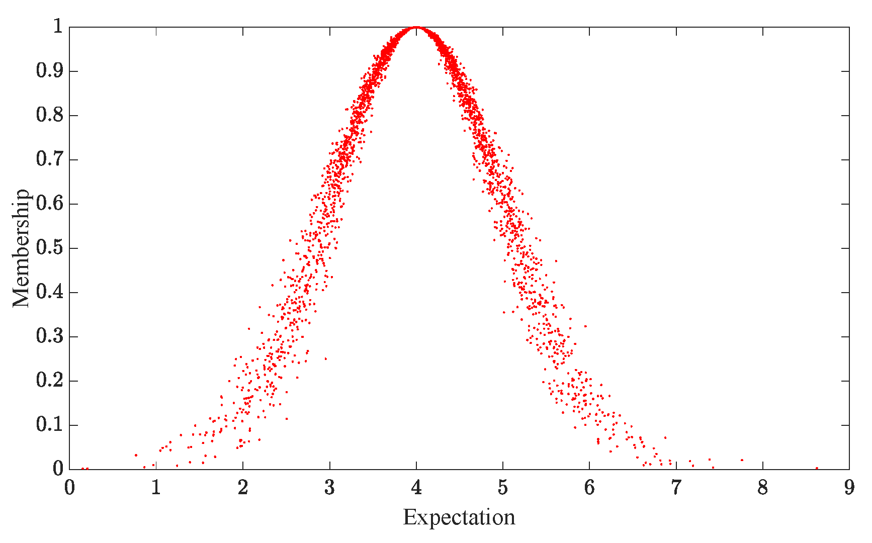
Figure 1. The cloud model concept.
Energies 17 01024 g001
Figure 2. (a) Original output of wind in the study area. (b) Original output of photovoltaic power in the study area. (c) Original output of hydropower in the study area.
Energies 17 01024 g002
Figure 3. (a) Output characteristics of wind. (b) Output characteristics of photovoltaic power. (c) Output characteristics of hydropower.
Energies 17 01024 g003
Figure 4. (a) Probability distribution of wind. (b) Probability distribution of photovoltaic power. (c) Probability distribution of hydropower.
Energies 17 01024 g004
Figure 5. Output cloud of the different wind power output intervals.
Energies 17 01024 g005
Figure 6. Output cloud of the different photovoltaic power output intervals.
Energies 17 01024 g006
Figure 7. Output cloud of the different hydropower output intervals.
Energies 17 01024 g007
Figure 8. (a) Kendall correlation coefficient of the Gaussian copula. (b) Spearman rank coefficient of the Gaussian copula.
Energies 17 01024 g008
Table 1. Cloud similarity value of every month.
Complementary SystemWind–PhotovoltaicWind–HydropowerPhotovoltaic–Hydropower
January29.9951.9101.881
February17.6682.3022.099
March29.7611.9571.927
April14.4172.4392.111
May12.7102.0181.780
June18.4651.9251.743
July12.3021.3771.242
August11.8911.2691.160
September27.2971.5961.513
October26.1201.8971.809
November23.9811.6651.635
December23.1821.3671.379
Table 2. Three-dimensional copula function of the goodness-of-fit test.
Copula FunctionRMSEAICBIC
Gaussian copula0.0138−75207759
t-copula0.0190−69657741
Disclaimer/Publisher’s Note: The statements, opinions and data contained in all publications are solely those of the individual author(s) and contributor(s) and not of MDPI and/or the editor(s). MDPI and/or the editor(s) disclaim responsibility for any injury to people or property resulting from any ideas, methods, instructions or products referred to in the content.