Medium- and Long-Term Power System Planning Method Based on Source-Load Uncertainty Modeling

Abstract

In order to consider the impact of source-load uncertainty on traditional power system planning methods, a medium- and long-term optimization planning method based on source-load uncertainty modeling and time-series production simulation is proposed. First, a new energy output probability model is developed using non-parametric kernel density estimation, and the spatial correlation of the new energy output is described using pair-copula theory to model the uncertainty analysis of the new energy output. Secondly, a large number of source-load scenarios are generated using the Markov chain Monte Carlo simulation method, and the optimal selection method for discrete state numbers is provided, and then the scenario reduction is carried out using the fast forward elimination technology. Finally, the typical time-series curves of the source-load uncertainty characteristics obtained are incorporated into the optimization planning method together with various flexible resources, such as the demand-side response and energy storage, and the rationality of the planning scheme is judged and optimized based on key indicators such as the cost, wind–light abandonment rate, and loss-of-load rate. Based on the above methods, this paper offers an example of the power supply planning scheme for a certain region in the next 30 years, providing effective guidance for the development of new energy in the region.

1. Introduction

Due to the volatility and stochastic nature of wind and solar resources, wind and solar power generation is characterized by uncertain, uncontrollable and unbalanced output. Under the new power system framework, the traditional power system planning method can no longer meet the needs of new energy development [1]. The uncertainty characteristics of source loads can affect the feasibility, economics, and environmental benefits of power system planning, and they need to be reasonably portrayed and dealt with by planning methods [2,3]. At the same time, from the perspective of the integration of the source network load storage, the medium- and long-term planning of the power system needs to take into account the distribution of wind and light resources, potential installed capacity, consumption, demand-side response, energy storage technology and other factors to optimize the allocation of various types of flexibility resources, improve the utilization rate of wind and light power generation and economic efficiency, and reduce the loss of wind and light abandonment and environmental pollution [4,5].

When the geographic locations of new energy stations are close to each other, the wind and solar resources in the region are similar, which makes the power outputs of the stations have correlation with each other. Scholars at home and abroad have utilized copula theory to portray the correlation of the power outputs between new energy stations [6,7,8]. The literature [9] proposed the theory of using the copula method to portray the correlation of random variables in the uncertainty analysis of new energy output and modeled the correlation of 15 wind farms in the Netherlands using the Gaussian copula. Other literature [10], on the other hand, pointed out that the simple use of the Gaussian copula is not capable of accurately portraying the correlation between wind farms and proposed the use of Archimedes copula clusters to portray the correlation between wind farms and photovoltaic plants. By comparing and analyzing the marginal distributions of the actual and forecasted power generation of new energy, a copula model was established to reveal the dependency structure between them. A multi-scenario forecasting modeling method based on this dependency relationship was then proposed in [11]. Subsequently, by analyzing the impact of forecasting deviations on the power supply balance and utilizing the patterns of forecasting deviations across different time periods in multiple scenarios, a method was proposed to incorporate the forecast credibility into the scheduling plans of provincial power grids.

A framework that integrates the K-means algorithm and the Monte Carlo method to generate a typical scenario set to describe the uncertainty of photovoltaic output and load is proposed in [12]. In order to describe the uncertainty of distributed generation and load, the literature [13] introduces the concept of interval numbers and solves the uncertain power flow through affine numbers. Sun Weiqing et al. constructed a polyhedron uncertainty set for the DG prediction error and determined the uncertainty of the DG output [14]. A method for typical output scenarios of multiple wind farms considering the spatiotemporal correlation is proposed in the literature [15]. The copula conditional distribution function is introduced to generate a dynamic scenario set with spatiotemporal correlation, which makes up for the shortcomings of existing scenario generation methods.

This type of method primarily describes uncertainty variables through uncertainty sets. The scenario reduction process for generating the set mainly focuses on extreme scenarios but weakens some high-expectation scenarios. Repeated coordination leads to the loss of some representative scenarios, which presents certain limitations. Although the above research effectively analyzes the correlation between wind and solar power, as well as the uncertainty of their output, it does not delve deeply into the dynamic changes in the temporal correlation of the joint distribution characteristics of wind and solar power, nor does it thoroughly explore scenario analysis in combination with uncertain output.

The existing new energy output data have problems such as insufficient data volume and insufficient record length, which make it difficult to reflect the temporal change characteristics and probability distribution characteristics of new energy sources [16,17,18]. At the same time, with the vigorous development of electric vehicles, home energy storage and other equipment resources, the volatility of the load increases, which will likewise have an impact on the power system [19,20,21]. Scenario analysis techniques can generate a large number of random scenarios that satisfy the characteristics of original uncertainty and randomness, effectively portraying the impact of various uncertainties in the power system [22,23]. The literature [24] proposed a scenario generation method for scenery based on a generative adversarial network (GAN). The literature [25] improved the generative adversarial network method and proposed the conditional generative adversarial network method, which solved the problem of the difficulty of modeling uncertainty in new energy to a certain extent, but it requires a large amount of high-quality data for training and it is difficult to assess the accuracy and diversity of the generated results. The literature [26] established a PV power plant output prediction model based on the ARMA model, but it only considers the case that the weather is sunny. The literature [27] established a real-time wind power output prediction model based on data mining and fuzzy clustering, but it needs to be based on a given wind speed and only real-time data can be obtained. The time-series method can fit the autocorrelation of the series better, but it cannot characterize the probability distribution of random variables over long time scales [28,29].

Aas et al. offered a detailed introduction to the pair-copula theory [30], the essence of which is that the joint density function of multivariate variables can be decomposed into the product of a series of binary copula density functions and marginal distribution functions according to a certain structure. The advantage is the flexibility of choosing different copula functions to fit different correlation structures without the limitation of a single copula function. The Markov chain Monte Carlo (MCMC) method is a dynamic simulation approach [31,32]. It combines Markov chains in stochastic processes (Markov chains) with traditional Monte Carlo sampling methods. Compared with the static simulation of the MC method, the sampling distribution of the MCMC method changes as the simulation proceeds, which can effectively characterize the temporal autocorrelation and probability distribution of the time series.

The contents of this paper can be mainly summarized as follows:

(1)

The tail fitting of the spatiotemporal joint probability distribution of the renewable energy output usually performs poorly. The spatial correlation of new energy output is modeled using the pair-copula theory; compared with the copula method, the effect of fitting the tails of the joint probability distribution is improved.

(2)

The scenario sets generated by existing scenario generation methods often exhibit significant homogeneity and are difficult to effectively reduce. Using the MCMC method for scene generation, the optimal discrete state number selection method is given, taking into account the temporal correlation of the new energy output; the scene reduction is carried out by using the fast predecessor elimination technique to obtain the typical scene of the source load.

(3)

Using the multi-scenario stochastic planning method to incorporate the impact of new energy uncertainty in power supply planning, it judges the reasonableness of the planning scheme and optimizes the adjustment based on the indicators of cost, the wind and light abandonment rate, and the lost load rate. It addresses the challenges faced in medium- to long-term power system planning under the coupling of source-load uncertainty.

2. Modeling the Spatial Correlation of New Energy Outputs

To reflect the spatial correlation of renewable energy output, we first use the non-parametric kernel density estimation method to model the probability of renewable energy output. Subsequently, the pair-copula method is employed to derive the joint probability distribution function of the renewable energy output.

2.1. Non-Parametric Kernel Density Estimation Method

Kernel density estimation is a non-parametric test method. This method does not need to assume the form of the probability distribution in advance, as the sample data can be obtained from the variable distribution characteristics. Let the sample of the random variable be $x_1,x_2\dots ,x_n$, then the kernel density estimate of the probability density function is:

$$\phi (x)={\displaystyle \frac{1}{nh}}{\displaystyle \sum _{j=1}^{n}K(\frac{x-x_j}{h})}$$

(1)

where n is the sample capacity; h is the bandwidth; and K is the kernel function. The types of kernel function are the uniform kernel function, triangular kernel function, gamma kernel function, Epanechnikov kernel, normal kernel and so on.

2.2. Pair-Copula Theory

Let $F\left(x_1,x_2,\dots ,x_n\right)$ be the joint distribution function with the marginal distribution $F_1(x_1),F_2(x_2),\dots ,F_n(x_n)$, then there exists a copula function $C:{[0,1]}^n\to [0,1]$ satisfying:

$$F\left(x_1,x_2,\dots ,x_n\right)=C\left(F_1(x_1),F_2(x_2),\dots ,F_n(x_n)\right)$$

(2)

If $F_1(x_1),F_2(x_2),\dots ,F_n(x_n)$ is continuous, then C is uniquely determined [32,33]. A partial derivation of both ends of the Equation (2) gives the joint density function as:

$$f\left(x_1,x_2,\dots ,x_n\right)=c\left(F_1(x_1),F_2(x_2),\dots ,F_n(x_n)\right){\displaystyle \prod _{i=1}^n{f}_i(x_i)}$$

(3)

where $f_i(x_i)$ is the edge density function and C is the copula density function, which can be expressed as:

$$c\left(F_1(x_1),F_2(x_2),\dots ,F_n(x_n)\right)={\displaystyle \frac{C\left(F_1(x_1),F_2(x_2),\dots ,F_n(x_n)\right)}{\partial F_1(x_1)\partial F_2(x_2)\dots \partial F_n(x_n)}}$$

(4)

The pair-copula theory decomposes a high-dimensional joint distribution into multiple two-dimensional distributions according to a certain structure, thus utilizing various two-dimensional copula functions to describe the correlation between different variables.

The formula derivation of the pair-copula is carried out using a ternary example. The joint density function of three variables can be decomposed using the conditional probability formula as:

$$f(x_1,x_2,x_3)=f(x_3)·f(x_2|x_3)·f(x_1|x_2,x_3)$$

(5)

For conditional probabilities $f(x_2|x_3)$ and $f(x_1|x_2,x_3)$, which satisfy:

$$f(x_2|x_3)=c_{23}(F_2(x_2),F_3(x_3))·f_2(x_2)$$

(6)

$$f(x_1|x_2,x_3)=c_{12|3}(F_{1|3}(x_1|x_3),F_{2|3}(x_2|x_3))·f(x_1|x_3)$$

(7)

Through Equations (5)–(7), the expression for the joint density function is given by:

$$f(x_1,x_2,x_3)=c_{12|3}(F_{1|3}(x_1|x_3),F_{2|3}(x_2|x_3))·c_{13}(F_1(x_1),F_3(x_3))·c_{23}(F_2(x_2),F_3(x_3)·{\displaystyle \prod _{k=1}^3{f}_k(x_k)}$$

(8)

The resulting iterative formula for the conditional probability density function for n variables is:

$$f(x|v)=c_{x{v}_j|v_{-j}}(F(x|v_{-j}),F(v_j|v_{-j}))·f(x|v_{-j})$$

(9)

The iterative formula for the conditional probability distribution function is:

$$F(x|v)={\displaystyle \frac{\partial C_{x,v_j|v_{-j}}(F(x|v_{-j}),F(v_j|v_{-j}))}{\partial F(v_j|v_{-j})}}$$

(10)

where $v_{-j}$ is the new vector obtained by removing element $v_j$ from $v$, and $C_{x,v_j|v_{-j}}$ is the copula distribution function.

For high-dimensional joint distributions, pair-copula decomposition exists in various structures, and the three main constructions are R-vine, C-vine, and D-vine. In general, C-vine is suitable for describing correlation structures with dominant variables, while D-vine is suitable for describing correlation structures with proximity relationships. A five-variable R-vine decomposition structure with four trees $T_i,i=1,2,3,4$ is shown in Figure 1.

The decomposition of the entire joint distribution consists of $n(n-1)/2$ edges and the marginal density function for each variable. The two most important steps of the pair-copula are the selection of the structure of the decomposition vine and the determination of the optimal binary copula for each.

3. Source-Load Bilateral Scene Generation and Reduction Methods

3.1. MCMC-Based Source-Load Scene Generation

A stochastic process is said to be Markov if it satisfies the requirement that its outcome at any moment depends on only the previous moment’s outcome and is independent of the outcome before that, and it is mathematically described as follows:

$$P[x(t_n)=x_n|x(t),t\le t_{n-1}]=P[x(t_n)=x_n|x(t_{n-1})]$$

(11)

By dividing all the values of the stochastic process $x(t)$ into N discrete states, the transfer probability matrix P can be obtained from the state transfer of the Markov chain, which quantifies the transfer probability properties of the Markov chain between different states [34,35,36]. The matrix remains unchanged during the state transfer process, and its i row and j column elements represent the probability of the Markov chain transferring from the previous state i to the next state j, as shown in Equation (12).

$$P(X_t=j|X_{t-1}=i)=p_{ij}$$

(12)

The autocorrelation coefficient (ACF) is the correlation coefficient between each moment in the time series and the data in a certain time interval before it, which is calculated as shown in Equation (13).

$$ACF(k)={\displaystyle \frac{\frac{1}{N-k}{\displaystyle \sum _{t=k+1}^N(x_t-\overline{x})(x_{t-k}-\overline{x})}}{\frac{1}{N}{\displaystyle \sum _{t=1}^N{(x_t-\overline{x})}^2}}}$$

(13)

The principle is to minimize the gap between the generated sequence and the original sequence ACD curve, as shown in Equation (14).

$$RSS={\displaystyle \sum _{i=1}^k{[AC{F}_0(i)-AC{F}_N(i)]}^2}$$

(14)

where $AC{F}_0$ is the $ACF$ curve of the original sequence, $AC{F}_N$ is the $ACF$ curve of the generated sequence, and k is the lag step of $ACF$.

The steps in the scene generation by the MCMC method are as follows:

(1)

Obtain the CDF probability distribution of the original sequence.

(2)

Delineate the discrete states and transform the original sequence into a state sequence.

(3)

Obtain the Markov transfer matrix P based on the state sequence P, and obtain the cumulative distribution matrix3 $P_{cum}$.

(4)

Generate random numbers between 0 and 1, and obtain the initial value according to the inverse distribution of the CDF of the original sequence, and further obtain the initial state.

(5)

Generate a random sequence according to the process in Figure 2.

(6)

After generating a certain length of random sequence, select the optimal number of discrete states N according to the RSS index, and then repeat steps 2–5 to obtain the final random sequence.

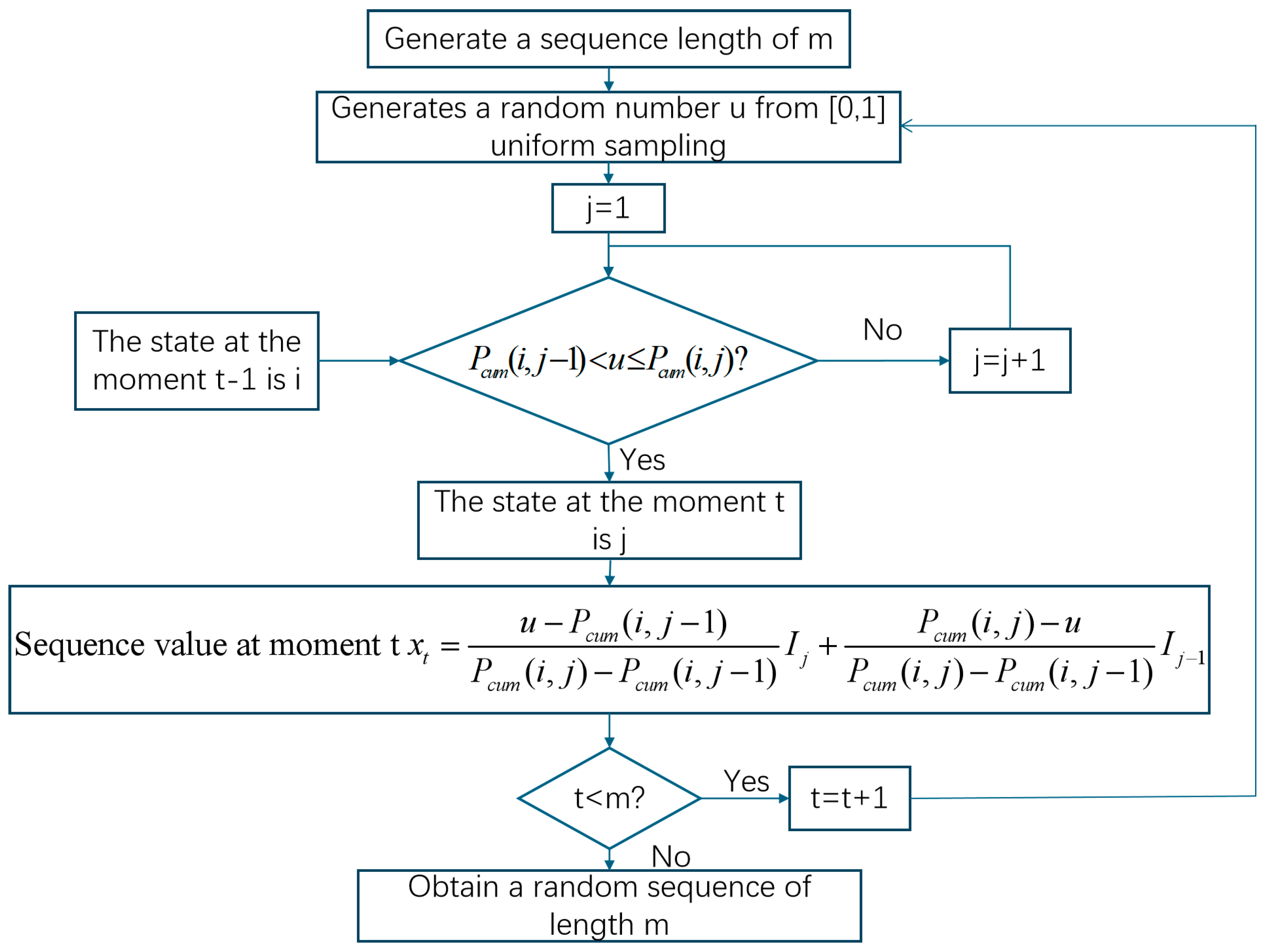
Figure 2. Flowchart for generating random sequences.

Figure 2. Flowchart for generating random sequences.

If there are multiple fluctuating sources in the power system, both temporal and spatial correlations need to be taken into account when performing scenario generation. Taking two fluctuating sources as an example, the conditional probability is:

$$P(X_{1,t}=j_1,X_{2,t}=j_2|X_{1,t-1}=i_1,X_{2,t-1}=i_2)$$

(15)

This can be obtained by solving Equations (16)–(18) using the pair-copula theory in Section 1:

$$\begin{array}{c}f(x_{1,t},x_{2,t}|x_{1,t-1},x_{2,t-1})=f(x_{1,t}|x_{1,t-1},x_{2,t-1})·\\ f(x_{2,t}|x_{1,t-1},x_{2,t-1})·c(F(x_{1,t}|x_{1,t-1},x_{2,t-1}),F(x_{2,t}|x_{1,t-1},x_{2,t-1}))\end{array}$$

(16)

$$\begin{array}{c}f(x_{1,t}|x_{1,t-1},x_{2,t-1})=c(F(x_{1,t}|x_{1,t-1}),\\ F(x_{2,t-1}|x_{1,t-1}))f(x_{1,t}|x_{1,t-1})\end{array}$$

(17)

$$F(x|v)={\displaystyle \frac{\partial C(F(x|v_{-j}),F(v_j|v_{-j}))}{\partial F(v_j|v_{-j})}}$$

(18)

3.2. Scene Reduction

The scene reduction method based on the fast antecedent elimination technique is more widely used. This method reduces the number of scenes by calculating the probabilistic distance between scenes and merging similar scenes into one representative scene. Compared with the K-means algorithm, the advantage of the fast prior generation elimination technique is that it is better for high-dimensional, noise-containing data; the selection of the initial clustering center of the K-means algorithm is random, which makes it difficult to determine the quality of its clustering convergence. Meanwhile, the scene obtained after cutting based on the fast antecedent elimination technique is the real time series, while the sequence obtained after K-means clustering is the average of the clusters, which will be smoother compared to the real sequence. The algorithm idea of the fast forward generation elimination technique is given below [37,38,39].

(1)

Compute the geometric distance between each pair of scenes s and s’ in the set of scenes S:

$$d(s,s^{\prime })=\sqrt{{\displaystyle \sum _{t=1}^T{(s(i)-s^{\prime }(i))}^2}}$$

(19)

(2)

Select the scene that minimizes the sum of the probability distances to the remaining scenes $s_m$:

$$z_d(s)=p_s{\displaystyle \sum _{u\in S\backslash \left\{s\right\}}{p}_{u}d(s,u)}$$

(20)

$$s_m=\arg \underset{s\in S}{\min } z_d(s)$$

(21)

where $p_s$ is the probability of scene s.

(3)

Replace the scene q with the scene q that has the closest probability distance from scene $s_m$ in the scene set S, add the probability of scene $s_m$ to the probability of scene q, and remove the scene from the scene set S:

$$q=\arg \underset{s\in S\backslash \left\{s_m\right\}}{\min }{p}_{s}d(s,s_m)$$

(22)

$$p_q=p_q+p_{s_m}$$

(23)

$$S=S\backslash \left\{s_m\right\}$$

(24)

(4)

If the number of scenes within the scene set S is greater than a given value, repeat steps 1–3; otherwise, complete the scene cut, where the remaining scenes in the scene set S are the cut scenes, and $p_s,s\in S$ is the probability of the scene.

4. Power Planning Model Based on Source-Load Uncertainty

4.1. Multi-Scenario Stochastic Planning Model

Compared with traditional planning, multi-scenario stochastic planning considers different scenarios, each representing a possible future situation, so it can more accurately assess the risk and feasibility of a scenario, leading to more reliable decisions. The mathematical model of multi-scenario stochastic planning is as follows:

$$\begin{array}{l}F=\min E(f(x,s))\\ s.t. h(x,s)\le 0,\forall s\in S\end{array}$$

(25)

where f is the objective function, h is the constraint function, x is the decision variable, s is the uncertain parameter, and S is the set of uncertain parameters. Each realization is called a scenario if S is discrete and takes a value in the range of $S=\{s_1,s_2\dots s_k\}$, corresponding to a probability of $p_1,p_2,\dots ,p_k$.

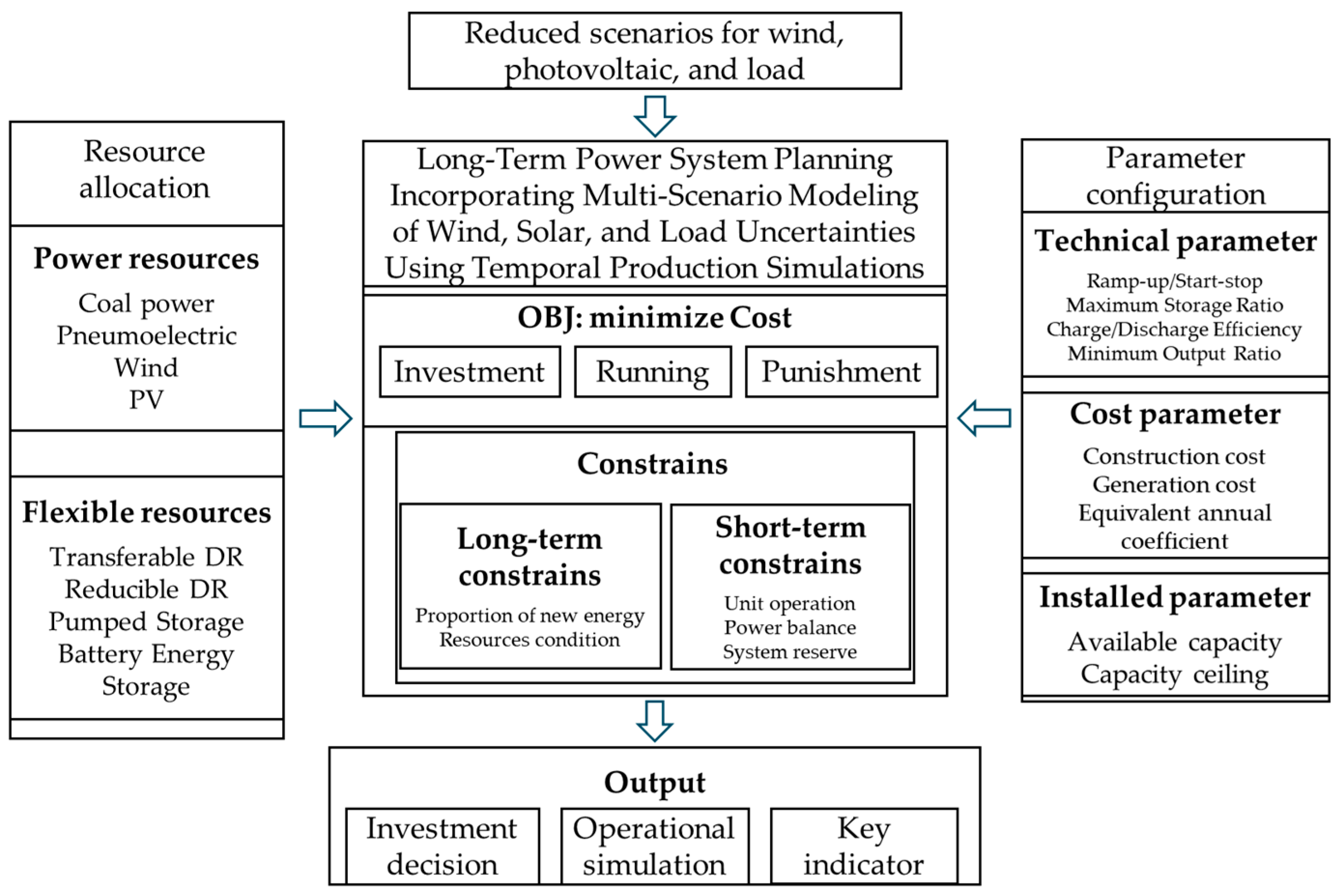
The process framework of the multi-scenario planning method is shown in Figure 3, including three parts: parameter input, optimization solution, and result output.

4.2. Optimization Planning Based on Time-Series Production Simulation

4.2.1. Objective Function

The objective of optimal planning based on time-series production simulation is to minimize the expected total system cost during the planning period with the following objective function:

$$F=\min C^{INV}+C^{OPR}+C^{PEN}$$

(26)

$$C^{INV}={\displaystyle \sum _{X}c(w,n^X)a^X{I}^X}$$

(27)

where $C^{INV}$ is the total system investment cost over the planning period; $X=\{G^{Gas},G^{Coal},W,PV,E{S}^{Battery},E{S}^{Hyrdo},D{R}^{Shed},D{R}^{Shift}\}$ is the set of types of generation and flexibility resources, which are, in order, coal, gas, wind, photovoltaic, battery storage, pumped storage, curtailable load demand response (hereinafter referred to as the curtailable DR), and transferable load demand response (hereinafter referred to as the transferable DR); $c(w,n^X)$ is the equivalent annual coefficient; $n_X$ is the benchmark discount rate; $n_X$ is the operating life of the resource; $a^X$ is the investment cost per unit of capacity of the resource $X$; and $a^X$ is the corresponding investment capacity of the resource $X$. $C^{OPR}$ is the total operating cost of the system during the planning period, which includes the generation cost of thermal power generating units and the load demand response cost, and $C^{PEN}$ is the penalty cost, which consists of the penalty cost for loss of load and penalty cost for abandonment of wind and solar energy.

4.2.2. Constraints

The constraints of the model mainly include resource capacity constraints, operation constraints, power balance constraints and standby constraints.

(1)

Landscape Scenario Generation Constraints

$$P_{s,t,w}^{The}={\overline{P}}_{s,t,w}^{The}{C}^W$$

(28)

$$P_{s,t,pv}^{The}={\overline{P}}_{s,t,pv}{C}^{PV}$$

(29)

${\overline{P}}_{s,t,w}^{The},{\overline{P}}_{s,t,pv}^{The}$ are the theoretical output values of wind power and photovoltaic under the scenario s moment t, while $C^W,C^{PV}$ are the installed capacities of wind power and photovoltaic.

(2)

Thermal power unit operation constraints

Thermal power units include coal power units and gas power units. For the overall planning of the region, thermal power units with similar output characteristics can be clustered, and the operation of the clustered thermal power units can be described by introducing three continuous variables, namely, start-up capacity, shutdown capacity, and online capacity, thus avoiding the introduction of 0–1 variables to describe the start-up and shutdown status of a single unit, which reduces the complexity of the model and effectively improves the solution rate.

$$O_{s,t,g}^Y{\alpha }_{\min }^Y\le P_{s,t,g}^Y\le O_{s,t,g}^Y{\alpha }_{\max }^Y$$

(30)

$$O_{s,t,g}^Y=O_{s,t-1,g}^Y+U_{s,t,g}^Y-D_{s,t,g}^Y$$

(31)

$$0\le D_{s,t+1,g}^Y\le O_{s,t,g}^Y-{\displaystyle \sum _{\tau =0}^{T_{on}^Y-1}{U}_{s,t-\tau ,g}^Y}$$

(32)

$$0\le U_{s,t+1,g}^Y\le C^Y-O_{s,t,g}^Y-{\displaystyle \sum _{\tau =0}^{T_{off}^Y-1}{D}_{s,t-\tau ,g}^Y}$$

(33)

$$P_{s,t,g}^Y-P_{s,t-1,g}^Y\le (O_{s,t,g}^Y-U_{s,t,g}^Y){\lambda }_{up}^Y+U_{s,t,g}^Y{\alpha }_{\min }^Y$$

(34)

$$P_{s,t-1,g}^Y-P_{s,t,g}^Y\le (O_{s,t,g}^Y-U_{s,t,g}^Y){\lambda }_{down}^Y$$

(35)

$U_{s,t,g}^Y,D_{s,t,g}^Y,O_{s,t,g}^Y$ are the start-up capacity, shutdown capacity, and online capacity of thermal power unit g at the scenario s moment t, respectively; $Y\in \{Gas,Coal\}$ denote the coal power unit and gas power unit, respectively; $C^Y$ is the installed capacity of the thermal power unit; ${\alpha }_{\min }^Y,{\alpha }_{\max }^Y$ are the ratio of the minimum and maximum outputs of thermal power unit g; and ${\lambda }_{up}^Y,{\lambda }_{down}^Y$ are the maximum value of the upward/downward climb rate of thermal power unit g. Equations (30) and (31) are the quantitative relationships among the start-up capacity, shutdown capacity, and online capacity; Equation (30) is the output constraint of thermal power unit g; Equation (31) is the quantitative relationship between the start-up capacity, shutdown capacity and online capacity; Equations (32) and (33) are the minimum start-up/shutdown time constraints of thermal power unit g; and Equations (34) and (35) are the ramp constraints of thermal power unit g.

(3)

Storage operation constraints

$$0\le P_{s,t,es}^{ES,dis},P_{s,t,es}^{ES,ch}\le C^{ES}$$

(36)

$$0\le E_{s,t,es}^{ES}\le C^{ES}{H}^{ES}$$

(37)

$$E_{s,t,es}^{ES}=E_{s,t-1,es}^{ES}+{\eta }^{ES,ch}{P}_{s,t,es}^{ES,ch}-{\displaystyle \frac{1}{{\eta }^{ES.dis}}}{P}_{s,t,es}^{ES,dis}$$

(38)

$${\displaystyle \sum _{s=1}^{N_s}{\rho }_s{\displaystyle \sum _{t=1}^T\left(P_{s,t,es}^{ES,dis}-P_{s,t,es}^{ES,ch}\right)}}=0$$

(39)

$Battery,Hydro$ denote the battery storage and pumped storage, respectively. $P_{s,t}^{ES,dis},P_{s,t}^{ES,ch}$ are the discharge power and charging power of the energy storage $ES$ in the scenario s at time t, respectively; $C^{ES}$ is the configured capacity of the energy storage $ES$; $E_{s,t}^{ES}$ is the energy state of the energy storage ES in the scenario s at time t; $H^{ES}$ is the maximum capacity–storage ratio of the energy storage ES; and ${\eta }^{ES.dis},{\eta }^{ES,ch}$ are the discharge efficiency and charging efficiency of the energy storage ES. Equation (36) is the energy storage charging and discharging power constraints; Equation (37) is the energy storage energy range constraints; and Equation (38) is the relationship between the energy and power storage constraints. Battery energy storage is a short-term energy storage, which needs to meet the charging and discharging power balance in each scene s, while pumped storage is a seasonal energy storage, which needs to meet the charging and discharging power balance in all the scenes.

(4)

Demand-side response constraints

$$0\le P_{s,t,d}^{Shed}\le C^{DR,Shed}$$

(40)

$$-C^{DR,Shift}\le P_{s,t,d}^{Shift}\le C^{DR,Shift}$$

(41)

$${\displaystyle \sum _{t=1}^T{P}_{s,t,d}^{Shift}}=0$$

(42)

$P_{s,t,d}^{Shed},P_{s,t,d}^{Shift}$ are the cuttable DR and transferable DR response power at scene s moment t, respectively; and $C^{DR,Shed},C^{DR,Shift}$ are the response capacity of cuttable DR and transferable DR, respectively. Equation (40) is the upper/lower limit constraint on the response power of the cuttable DR; Equation (41) is the upper/lower limit constraint on the response power of the transferable DR. For the transferable DR, it is necessary to satisfy that the load increase and decrease in each scene s are equal, as shown in Equation (42).

5. Simulation Example

To verify the effectiveness of the method proposed in this paper, simulation analysis was conducted using actual power source and load data from a specific region in China. The data resolution was 15 min, with a time span of one year.

5.1. Spatial Correlation of New Energy Power

Here is a case study involving three wind farms in a specific region within China, with installed capacities of 148.5 MW, 52.5 MW, and 54.9 MW, respectively.

The probabilistic modeling of the wind farms’ power output is conducted using the mixed Gaussian distribution, the Weibull distribution, and kernel density estimation methods, the outcomes of which are presented as

Table 1. Root mean square error value of the output fitting curve of the wind farms.

Probabilistic Modeling	Root Mean Square Error
Kernel Density Estimation	0.1436
Weibull Distribution	0.2126
Mixed Gaussian Distribution	0.2847

.

Calculate the Kendall correlation coefficients among the three wind farms, and further derive the copula functions between each pair of wind farms. The matrix corresponding to the decomposed vine structure is:

$$A=\left(\begin{array}{ccc}3& 3& 2\\ 0& 2& 3\\ 0& 0& 1\end{array}\right)$$

(43)

The matrix composed of the three selected optimal bivariate copula functions is:

$$family=\left(\begin{array}{cc}frank& 0\\ surclayton& frank\end{array}\right)$$

(44)

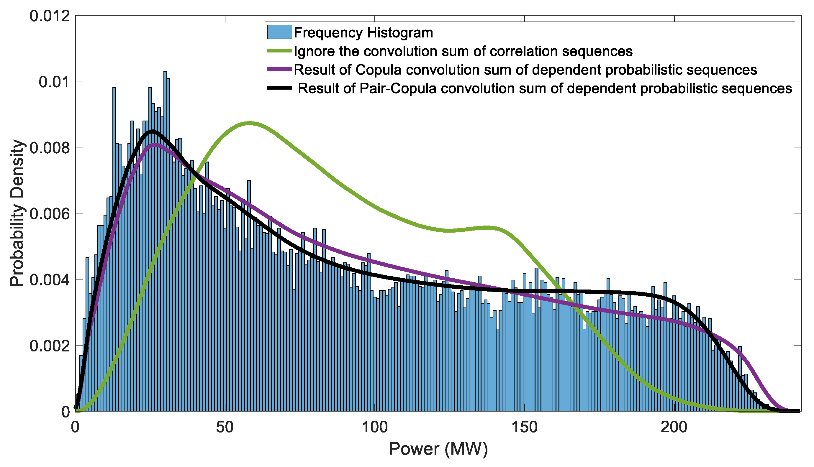
The Frank copula fitting joint probability distribution is shown in Figure 4. Using the theory of dependent probabilistic sequence operations, the probability distribution of the total output from the three wind farms is calculated, as shown in Figure 5. In the figure, the purple line represents the result calculated using the pair-copula method, and the black line represents the result obtained using the high-dimensional copula method. For comparison, the figure also includes a histogram depicting the actual total output probability statistics, and the green line represents the result obtained without considering the correlation between the wind farms, achieved simply by the convolution of the marginal distributions. As can be seen from the calculation results in Figure 5, both the high-dimensional copula and pair-copula methods yield total output probability distributions that are in good agreement with the actual total output probability distribution. Moreover, the pair-copula method provides a better fit to the tails of the output distribution curve. This research result shows that the pair-copula method can be used as a priority in the probabilistic modeling of wind power output uncertainty. By better fitting the probability characteristics of wind and solar power, the uncertainty of the renewable energy output faced by the medium- and long-term planning of the power system can be reduced and the confidence in the boundaries of the input data can be improved.

The quantitative evaluation using the K-S test for the results obtained by the three methods is shown in

Table 2. K-S test results of the wind farm total output probability distribution.

Method	p-Value	Significance Level	Results
Copula	1.3699	0.05	Pass
Pair-Copula	1.6933	0.05	Pass

. It can be observed that both the high-dimensional copula and the pair-copula methods pass the K-S test, with the pair-copula exhibiting a better fitting performance.

5.2. Generation and Reduction of Source-Load Scenarios

Based on wind power, photovoltaic, and load data from 2017, generate scenarios for the wind, solar, and load for the next 30 years, and perform a scenario reduction to obtain the typical source-load scenarios. Set the number of typical wind power scenarios to seven, the number of typical photovoltaic scenarios to eight, and the number of typical load scenarios to three.

Generate random sequences of a certain length separately for the wind power, photovoltaic (PV), and load in advance. Calculate the autocorrelation function (ACF) curves. The lag length for wind power is selected as 48, which is 12 h; the lag lengths for PV and load are selected as 96, which is 24 h.

Table 3. RSS index of the ACF curves of the wind power, PV, and load under different discrete state numbers.

Discrete State Number	RSS Index of ACF Curves
	Wind Power	PV	Load
10	0.0589	0.6593	0.0789
20	0.0383	0.0692	0.0464
30	0.0843	0.0860	0.0421
40	0.1033	0.1883	0.0421
50	0.1305	0.2784	0.0771
60	0.1453	0.3658	0.0827

presents the root sum square (RSS) indicators of the ACF curves for the wind power, PV, and load under different numbers of discrete states. Based on the calculation results, the discrete state numbers for wind power and photovoltaic are selected as 20, and the discrete state number for load is selected as 30.

The Kolmogorov–Smirnov (K-S) test is utilized to verify if the generated sequences comply with the probability characteristics of the original sequences. The K-S test statistics and corresponding p-value for the wind power, photovoltaic (PV) power, and load are presented in

Table 4. K-S test results of the generated sequences of wind power, photovoltaic and load.

Category	p-Value	Significance Level	Results
Wind power	1.9443	0.05	Pass
Photovoltaic	1.8591	0.05	Pass
Load	1.8822	0.05	Pass

. It can be observed that the generated sequences for the wind power, PV power, and load all pass the K-S test, indicating that they satisfy the probability characteristics of the original sequences. By reducing massive scenes through rapid predecessor elimination technology, we can solve the dimensionality disaster problem caused by too many scenes and improve the planning efficiency.

Figure 6, Figure 7 and Figure 8 showcase the curtailed typical scenarios of wind power, photovoltaics, and load based on the fast forward elimination technique, and they provide the probability of each scenario. Through probabilistic scenario generation and reduction technology, the size of the scenario set space can be effectively controlled, and at the same time, the power system planning boundaries under different confidence levels can be given in a targeted manner according to the probability of scenario occurrence.

5.3. Power Planning

Considering the construction progress of the new power system and the utilization rate of new energy consumption, calculations are carried out for six scenarios: three with new energy installed capacity penetration rates of 50%, 60%, and 70%, respectively, and each of these under two conditions—with and without wind curtailment and solar curtailment penalties. Let scenario 1, scenario 2, and scenario 3 represent the cases with new energy installed capacity penetration rates of 50%, 60%, and 70%, respectively, and without wind curtailment and solar curtailment penalties. Let scenario 4, scenario 5, and scenario 6 represent the cases with new energy installed capacity penetration rates of 50%, 60%, and 70%, respectively, but with wind curtailment and solar curtailment penalties. The planning schemes calculated for these six scenarios are shown as in

Table 5. Power planning schemes under scenarios 1–6.

Category/MW	Scenario 1	Scenario 2	Scenario 3	Scenario 4	Scenario 5	Scenario 6
New Coal Power	10,803	10,150	9963.2	10,545	10,182	10,053
New Pneumoelectric	384.7	946.2	1034.3	569.8	843.6	325.4
New Wind Power	10,551	10,236	10,631	9798.4	7435.6	6979.4
New Photovoltaic	3537.2	10,958	22,329	4216.5	13,653	24,538
New Demand Response	874.7	874.7	874.7	874.7	874.7	874.7
New Demand Response	874.7	874.7	874.7	874.7	874.7	874.7
New Battery Energy Storage	389.6	389.6	679.8	389.6	1096.6	1749.3
New Pumped Storage	0	0	0	0	244.7	1649.3
Total Coal Power	13,803	13,150	12,963	13,545	13,182	13,053
Total Pneumoelectric	684.7	1246.2	1334.3	869.8	1143.6	625.4
Total Wind Power	10,684	10,369	10,764	9931.4	7568.6	7112.4
Total Photovoltaic	3804.2	11,225	22,596	4483.5	13,920	24,805
Total Demand Response	874.7	874.7	874.7	874.7	874.7	874.7
Total Demand Response	874.7	874.7	874.7	874.7	874.7	874.7
Total Battery Energy Storage	389.6	389.6	679.8	389.6	1096.6	1749.3
Total Pumped Storage	100	100	100	100	344.7	1749.3

.

The planning schemes obtained from scenarios 1 to 6 are analyzed according to the criteria proposed in Section 3, and the results are shown in

Table 6. Indicators of planning schemes under scenarios 1–6.

Indicators	Scenario 1	Scenario 2	Scenario 3	Scenario 4	Scenario 5	Scenario 6
Total Cost (Million dollars)	2938.9	2991.4	3152.8	2948.6	3100.0	3594.6
Curtailment Rate (%)	1.63	6.34	17	0.03	0.69	1.9
Load Loss Rate (%)	0.0006	0.0015	0.0044	0.0013	0.0036	0.05

.

From the table, it is evident that as the penetration rate of new energy installations increases, the total planning cost rises, and the difference between the total planning cost with and without curtailment penalties becomes significantly larger.

When the penetration rate of new energy installations reaches 70%, the curtailment rate would be as high as 17% without curtailment penalties. The issue of new energy consumption can be addressed by incorporating curtailment penalties into the planning process. It can be seen from the table that after considering the wind curtailment penalties, the wind curtailment rate drops dramatically: at new energy installation penetration rates of 50%, 60%, and 70%, the curtailment rates fall from 1.63%, 6.34%, and 17%, respectively, to 0.03%, 0.69%, and 1.9%, effectively enhancing the capacity for new energy consumption.

However, after considering the penalty costs for the curtailed wind and solar power, the loss of load probability (LOLP) has seen a certain increase, particularly with a renewable penetration rate of 70%, where the LOLP rises from 0.0044% to 0.05%, an increase of more than tenfold. An excessively high LOLP may cause instantaneous fluctuations in the grid voltage and frequency, potentially endangering the entire power system, hence the need to impose limits on the LOLP. Aside from directly capping the LOLP, it can also be reduced by increasing the upper limit of flexible resource installations and raising the penalty costs for load loss.

Under a renewable installation capacity penetration rate of 70% and considering the penalties for curtailed wind and solar power, different conditions are added to the original scenario 6 to reduce the LOLP, resulting in scenarios 7 through 11. Scenario 7 adds an LOLP constraint to scenario 6; scenario 8 increases the energy storage capacity limit from 10% to 20% on top of scenario 7; scenario 9 raises the demand-side response limit from 5% to 10% on scenario 8; scenario 10 doubles the load loss penalty cost from 1428 MWh to 2856 MWh on scenario 9; and scenario 11 reintroduces the LOLP constraint on top of scenario 10.

Table 7. Indicators of planning schemes under scenarios 6–11.

Indicators	Scenario 6	Scenario 7	Scenario 8	Scenario 9	Scenario 10	Scenario 11
Load Rate Constraints (0/1)	0	1	0	0	0	1
Upper Limit of DR	0.05	0.05	0.05	0.1	0.1	0.1
Upper Limit of Storage	0.1	0.1	0.2	0.2	0.2	0.2
Load Loss Penalty Cost ($/MWh)	1428	1428	1428	1428	2856	2856
LOLP (${10}^{-3}\%$)	50.18	0.13	16.93	5.08	1.59	0.13
Wind Curtailment Rate (%)	5.86	7.84	2.34	1.44	1.42	0.01
Solar Curtailment Rate (%)	0.89	1.52	0.03	0.013	0.014	0
Transferable DR (MW)	874.7	874.7	874.7	1749.3	1749.3	1749.3
Reducible DR (MW)	874.7	874.7	874.7	1749.3	1749.3	1749.3
Battery Energy Storage (MW)	1749.3	1749.3	3498.7	3269.4	3465.3	3498.7
Pumped Storage (MW)	1749.3	1749.3	3498.7	1686.1	1691.6	1827.1
Cost (Million dollars)	3594.6	3674.9	3526.2	3350.9	3355.0	3361.5

presents the LOLP and other indicators under the conditions of scenarios 6 through 11.

Against the backdrop of scenario 6, the load ratio has plummeted to 0.00013%, but flexible resources still touch the ceiling of the installed capacity, with both the wind spillage and total cost on the rise. Essentially, scenario 7 merely adjusts to compress the renewable energy output to meet the under-load ratio criteria. In scenario 8, contrasted with scenario 6, the under-load ratio has dipped to 0.01693%, falling short of the under-load ratio requirement, and the storage capacity has also hit the upper limit, signaling that the system’s flexibility is still inadequate under this scenario. Scenario 9, in comparison to scenario 8, shows a further decline in wind spillage, with the under-load ratio settling at 0.00508% and the storage capacity not reaching its peak, suggesting that the system’s flexibility is now sufficient and the under-load ratio’s failure to meet the requirement might be due to inadequate penalties for under-load situations. Scenario 10, juxtaposed against scenario 9, observes the under-load ratio to be reduced to 0.00159%, nearly meeting the under-load ratio requirement, and sees a marked decrease in the total planning cost and wind spillage rate compared to scenarios 6 and 7, illustrating that the energy storage and demand-side response cannot only boost system flexibility and integrate renewable energy but also enhance the system’s economic performance. Scenario 11 sees an increase in the installed capacity of flexibility resources compared to scenario 10. Finally, comparing scenario 11 and scenario 7 reveals that scenario 11 experiences a significant drop in the planning cost and wind spillage rate, highlighting the pivotal status of flexibility resources in future power systems characterized by high proportions of renewable energy.

6. Conclusions

The biggest problem facing medium- and long-term power system planning is the high uncertainty of source loads and their mutual coupling. The new energy output probability distribution fitting method and operation scenario probabilistic generation technology proposed in this paper can provide boundary conditions with higher credibility for medium- and long-term power system planning and improve the confidence level of the planning results.

The output of the new energy sources model is built in this paper, and a joint probability distribution model for new energy output that accounts for spatial correlation is established. It proposes a method for source-load bilateral scenario generation and curtailment that considers temporal correlation, deriving typical source-load bilateral scenarios. It also presents a method for power system production sequence simulation using multi-scenario stochastic programming, with critical indicators used to evaluate the planning schemes. The conclusions of this study are as follows:

(1)

The pair-copula method provides a better fit for new energy output, making it more adaptable to the uncertainty of new energy output.

(2)

The scenario reduction method based on the fast forward sweep technique effectively reduces the number of scenarios while providing the probability of each scenario.

(3)

The planning results indicate that flexible resources can significantly reduce the curtailment rate of new energy and the loss of load probability, playing an irreplaceably important role in future power systems with a high proportion of new energy.

References

1. Yao, Z.; Wang, Z. A two-level collaborative optimization configuration method for integrated energy systems considering wind and solar uncertainties. Power Syst. Technol. 2020, 44, 4521–4531. [Google Scholar]
2. Ma, N.; Liu, G.; Wu, J.; Wang, Y.; Xin, L.; Peng, Q. Collaborative Optimization Model for “Source Storage” Capacity Configuration for Carbon Emissions [J/OL]. Southern Power System Technology. pp. 1–11. Available online: http://kns.cnki.net/kcms/detail/44.1643.tk.20240701.1519.005.html (accessed on 29 July 2022).
3. Dou, Z.; Zhang, C.; Duan, C.; Wen, X.; Sun, C. Multi-time scale economic regulation model of virtual power plant considering multiple uncertainties of source, load and storag. J. Comput. Methods Sci. Eng. 2024, 24, 935–953. [Google Scholar] [CrossRef]
4. Yuan, Z.; Zhang, H.; Cheng, H.; Zhang, S.; Zhang, X.; Lu, J. Low-carbon oriented power system expansion planning considering the long-term uncertainties of transition tasks. Energy 2024, 307, 132759. [Google Scholar] [CrossRef]
5. Liu, D. Planning strategy for new energy systems in distribution networks considering source load uncertainty. Guangdong Electr. Power 2023, 36, 77–83. [Google Scholar]
6. Li, J.; Chen, J.; Chen, Z.; Nie, Y.; Xu, A. Short-term wind power forecasting based on multi-scale receptive field-mixer and conditional mixture copula. Appl. Soft Comput. 2024, 164, 112007. [Google Scholar] [CrossRef]
7. Hu, K.; Fu, Z.; Lang, C.; Li, W.; Tao, Q.; Wang, B. Short-Term Photovoltaic Power Generation Prediction Based on Copula Function and CNN-CosAttention-Transformer. Sustainability 2024, 16, 5940. [Google Scholar] [CrossRef]
8. Moradian, S.; Gharbia, S.; Iglesias, G.; Olbert, A.I. A copula post-processing method for wind power projections under climate change. Energy Convers. Manag. X 2024, 23, 100660. [Google Scholar] [CrossRef]
9. Papaefthymiou, G.; Kurowicka, D. Using Copulas for Modeling Stochastic Dependence in Power System Uncertainty Analysis. IEEE Trans. Power Syst. 2009, 24, 40–49. [Google Scholar] [CrossRef]
10. Valizadeh Haghi, H.; Tavakoli Bina, M.; Golkar, M.A.; Moghaddas-Tafreshi, S.M. Using Copulas for analysis of large datasets in renewable distributed generation: PV and wind power integration in Iran. Renew. Energy 2010, 35, 1991–2000. [Google Scholar] [CrossRef]
11. Sun, X.; Ma, X.; Zhang, X. Dependence Relationship Based Scenario Generation of Power Prediction for Renewable Energy and Its Application in Dispatch. Autom. Electr. Power Syst. 2019, 43, 10–17+44. [Google Scholar]
12. Ma, W.; Gao, H.; Yang, Y.; Wang, C.; Pan, H.; Liu, Y.; Liu, J. Two-stage optimal operation for distribution network based onfast identification of reconfiguration level. Proc. CSEE 2022, 42, 5154–5168. [Google Scholar]
13. Gao, C.; Yu, A.; Ding, Y. Multi-period dynamicreconfiguration of active distribution network based on improved recursive ordered clustering. Electr. Power Autom. Equip. 2021, 41, 84–90. [Google Scholar]
14. Sun, W.; Liu, W.; Zhang, J. Collaborative optimization for dynamic reconfiguration of distribution network and mobile energy storage in background of high proportion of renewable energy. Autom. Electr. Syst. 2021, 45, 80–90. [Google Scholar]
15. Zhao, S.; Jin, T.; Li, Z.; Liu, J.; Li, Y. Wind power scenariogeneration for multiple wind farms considering tempora!and spatial correlations. Power Syst. Technol. 2019, 43, 3997–4004. [Google Scholar]
16. Zhu, Z.; Yuan, W.; Wu, Y.; Yang, X.; Chen, G. A missing data filling method for power grid based on historical data mining assisted scenario analysis. Electr. Autom. 2023, 45, 72–74. [Google Scholar]
17. Zhang, S.; Chen, S.; Lin, F.; Zhao, X.; Li, G. Collaborative optimization and scheduling of source, load and storage of distribution networks considering distributed energy and load uncertainty. J. Phys. Conf. Ser. 2024, 2823, 012031. [Google Scholar] [CrossRef]
18. Zhang, Z.; Yang, S.; Ma, Y.; Sun, S.; Yu, P.; Yang, F. Constrained distributionally robust optimization for day-ahead dispatch of rural integrated energy systems with source and load uncertainties. Front. Energy Res. 2024, 12, 1411152. [Google Scholar] [CrossRef]
19. Sheng, D.; Gao, H.; Long, Y. Ordered charging strategy considering load forecasting in residential scenarios. Guangdong Electr. Power 2023, 36, 70–78. [Google Scholar]
20. Shi, S.; Wang, P.; Zheng, Z.; Zhang, S. Two-Layer Optimization Strategy of Electric Vehicle and Air Conditioning Load Considering the Benefit of Peak-to-Valley Smoothing. Sustainability 2024, 16, 3207. [Google Scholar] [CrossRef]
21. Wei, C.; Xu, J.; Liao, S.; Sun, Y. Aggregation and Scheduling Models for Electric Vehicles in Distribution Networks Considering Power Fluctuations and Load Rebound. IEEE Trans. Sustain. Energy 2020, 11, 1. [Google Scholar] [CrossRef]
22. Nie, Y.; Shi, G. Research on Demand and Scenario Analysis of Big Data Application in Intelligent Distribution Network. China Plant Eng. 2021, 22, 23–25. [Google Scholar]
23. Kishita, Y.; Yamaguchi, Y.; Mizuno, Y.; Fukushige, S.; Umeda, Y.; Shimoda, Y. Scenario Analysis of Electricity Demand in the Residential Sector Based on the Diffusion of Energy-Efficient and Energy-Generating Products. Sustainability 2024, 16, 6435. [Google Scholar] [CrossRef]
24. Li, K.; Zhang, Z.; Wang, F.; Jiang, L.; Zhang, J.; Yu, Y.; Mi, Z. An independent microgrid capacity stochastic optimization configuration model based on GAN scenario simulation and conditional value at risk. Power Syst. Technol. 2019, 43, 1717–1725. [Google Scholar]
25. Dong, X.; Sun, Y.; Pu, T. A method for generating renewable energy scenarios based on conditional generative adversarial networks. Proc. CSEE 2020, 40, 5527–5536. [Google Scholar]
26. Yan, H.; Zhang, J.; Hu, Y.; Zhang, L.; Jiao, T. Distributed Photovoltaic Power Generation Output Prediction Based on Spatial Correlation and Error Evaluation Indexes. Zhejiang Electr. Power 2020, 39, 54–60. [Google Scholar]
27. Shi, H.; Zhang, Z.; Ding, M.; Pan, J. Research on Wind Power Prediction Method Based on Similarity Index Clustering. Comput. Integr. Manuf. Syst. 2022, 39, 121–125. [Google Scholar]
28. Cui, L.; Zhou, Y.; Shi, J.; Gao, Y.; Yan, L. Method of MCMC wind power sequence modeling based on climbing direction state division. Mod. Electron. Tech. 2024, 47, 113–120. [Google Scholar]
29. Sun, Z.; Song, D.; Peng, Q.; Li, H.; Li, P. Improving long-term electricity time series forecasting in smart grid with a three-stage channel-temporal approach. J. Clean. Prod. 2024, 143051. [Google Scholar] [CrossRef]
30. Aas, K.; Czado, C.; Frigessi, A.; Bakken, H. Pair-copula constructions of multiple dependence. Insur. Math. Econ. 2009, 44, 182–198. [Google Scholar] [CrossRef]
31. Liu, D.; Wang, W.; Liu, B.; Zhang, H.; Gang, Q.; Hao, H.; Li, G.; Xiao, G. Application of Markov Modified Combination Model Mid-long Term Available Quantity of Electricity Forecasting in Xinjiang Wind Power. Power Syst. Technol. 2020, 44, 3290–3297. [Google Scholar]
32. Hirt, M.; Kreouzis, V.; Dellaportas, P. Learning variational autoencoders via MCMC speed measures. Stat. Comput. 2024, 34, 164. [Google Scholar] [CrossRef]
33. Zhao, Y.; Liu, Q.; Kuang, J.; Xie, K.; Du, W. Modeling multivariate dependence by nonparametric pair-copula construction in composite system reliability evaluation. Int. J. Electr. Power Energy Syst. 2021, 124, 106373. [Google Scholar] [CrossRef]
34. Chen, F.; Wang, H.; Liu, H.; Zhao, M.; Zhang, X.; Gao, H. Temporal-spatial correlation modeling of wind speeds in multiple wind farms based on improved Pair-Copula method. Renew. Energy Resour. 2023, 41, 60–66. [Google Scholar]
35. Zhu, C.; Zhang, Y.; Yan, Z.; Zhu, J. A Nested MCMC Method Incorporated with Atmospheric Process Decomposition for Photovoltaic Power Simulation. IEEE Trans. Sustain. Energy 2020, 11, 2972–2984. [Google Scholar] [CrossRef]
36. Chao, H.; Hu, B.; Xie, K.; Tai, H.-M.; Yan, J.; Li, Y. A Sequential MCMC Model for Reliability Evaluation of Offshore Wind Farms Considering Severe Weather Conditions. IEEE Access 2019, 7, 132552–132562. [Google Scholar] [CrossRef]
37. Xu, S.; Ai, X.; Zou, J.; Zhang, S.; Li, P.; Huang, Y.; Wen, J. Application of optimizing state number Markov chain Monte Carlo algorithm in wind power generation. Electr. Power Autom. Equip. 2019, 39, 61–68. [Google Scholar]
38. Huang, Y.; Zhou, X.; Guo, H.; Wang, D.; Xie, J. Power Regulation Strategy of Wind-Solar-Hydrogen Coupling SystemBased on Parameter Adaptive Stochastic Model Predictive Control. J. Chin. Soc. Power Eng. 2024, 44, 1109–1117. [Google Scholar]
39. Growe-Kuska, N.; Heitsch, H.; Romisch, W. Scenario reduction and scenario tree construction for power management problems. In Proceedings of the 2003 IEEE Bologna Power Tech Conference Proceedings, Bologna, Italy, 23–26 June 2003; Volume 3, pp. 1–7. [Google Scholar] [CrossRef]
Figure 1. An R-vine structure with five variables, four trees, and ten edges.
Energies 17 05088 g001
Figure 3. The process framework diagram of the multi-scenario planning.
Energies 17 05088 g003
Figure 4. Frank copula fitting joint probability distribution diagram.
Energies 17 05088 g004
Figure 5. Comparison of the total output probability distribution and actual results of the three wind farms.
Energies 17 05088 g005
Figure 6. Typical scenarios of wind power.
Energies 17 05088 g006
Figure 7. Typical scenarios of photovoltaic.
Energies 17 05088 g007
Figure 8. Typical scenarios of load.
Energies 17 05088 g008