Abstract
When colloidal particles are deposited in a heat transfer channel, they increase the flow resistance in the channel, resulting in a substantial decrease in heat transfer efficiency. It is critical to have a comprehensive understanding of particle properties in heat transfer channels for practical engineering applications. This study employed the Reynolds stress model (RSM) and the discrete particle model (DPM) to simulate particle deposition in a 3D corrugated rough-walled channel. The turbulent diffusion of particles was modeled with the discrete random walk model (DRW). A user-defined function (UDF) was created for particle–wall contact, and an improved particle bounce deposition model was implemented. The research focused on investigating secondary flow near the corrugated wall, Q-value standards, turbulent kinetic energy distribution, and particle deposition through validation of velocity in the tube and particle deposition modeling. The study analyzed the impact of airflow velocity, particle size, corrugation height, and corrugation period on particle deposition efficiency. The findings suggest that the use of corrugated walls can significantly improve the efficiency of deposition for particles less than 20 μm in size. Specifically, particles with a diameter of 3 μm showed five times higher efficacy of deposition with a corrugation height of 24 mm compared to a smooth surface.
1. Introduction
Heat exchangers are widely used in power generation and in heating, ventilation, and air conditioning (HVAC) systems in everyday life and industrial production. After a long period of use, dirt deposits tend to form on the surface of a heat exchanger, which affects the heat transfer efficiency of the heat exchanger. In the case of HVAC systems, such fouling also affects indoor air quality (IAQ), and when the particle size (dp) is less than 2.5 μm, particulate matter enters the human body through the respiratory tract, posing a serious threat to human health [1]. Since most people spend most of their time indoors [2], the study of particle motion characteristics in heat exchangers has received much attention.
The structure of the heat exchanger is a key factor influencing the heat transfer performance and particle deposition characteristics. Smooth-walled heat exchangers have been studied more comprehensively [3,4,5]. Lai et al. [6,7] suggested the addition of low ribs to enhance particle deposition in the pipe and to control the number of particles in the pipe wall by periodic cleaning through removable sections. By using the CFD approach, Lu and Lu [8] investigated how rib shape affected particle deposition in turbulent pipes. The impacts of square, triangular, and circular fins on particle deposition were examined. It was found that different rib shapes have a great influence on particle deposition and also produce different resistance. Lu and Quan [9] discussed particle deposition in 3D ribbed channels under different conditions. Bi et al. [10] compared and analyzed the influence of micro-dimpled channels, cylindrical grooved channels, and low-ribbed channels on fluid pressure loss through the field synergy theory. It was found that the micro-dimpled channel and the cylindrical grooved channel had less fluid resistance than the low-ribbed channel. Curved ribs significantly reduce the energy loss of a pipe compared to rectangular ribs. Han and Lu [11] investigated the deposition of particles on the walls of dimple-like concave sockets and explored the effects of different dimple depth-to-inner diameter ratios as well as dimple inner diameter-to-dimple spacing ratios on the deposition of different particles and found that deposition was facilitated for particles smaller than 10 μm in size and had little or no effect on particles larger than 10 μm in size. Andaz and Maso [12] investigated the deposition of particles in a ribbed channel after the addition of a deflector using the Launder, Reece, and Rodi (LRR) model [13] and the Lagrange model and found that the deposition rate of particles with a particle size of 50 μm increased by 148.36%. Another hotspot for the study of fluid–solid coupling in heat exchangers is the study of nanofluids with heat exchangers. In this area, the research of Ben Hamida’s team is more comprehensive and influential. Ben Hamida et al. [14] conducted a numerical analysis of the thermal management of light-emitting diode packages. They simulated the heat dissipation process from an LED chip to the heat sink. To increase the junction temperature of a square LED lamp, square and circular holes were drilled in the center of the heat sink. The researchers found that the junction temperature decreased with an increase in the internal surface of the hole. Ben Hamida et al. [15] used the Galerkin finite-element method (GFEM) to simulate the heat transfer process inside a hybrid nanofluid-filled channel under the action of an electric field. The effect of fin geometry on heat transfer was investigated using the central composite design (CCD) method. The results showed that each increase of 0.01 in nanoparticle concentration increased the Nusselt number by 5.19%. In addition, the effect of using nanofluids in a two-tube heat exchanger with an axial spoiler on the heat transfer rate and pressure drop in a turbulent flow regime has been investigated [16]. The problem of magnetohydrodynamic nonconstant natural convection heat transfer in a circular shell with four heated cylinders in each of the horizontal and vertical midplanes was investigated using a two-dimensional numerical computational method [17]. The efficiency of carbon nanotube (CNT)-50% water +50% ethylene glycol nanofluid in a corrugated finned tilted box radiator under Lorentz force was investigated by numerical simulation considering the nanofluid radiation effect [18]. Corrugated wall piping is one of the more common types of piping used in engineering to enhance heat transfer efficiency and save energy. Russ and Beer [19] discussed the effect of pipes with sinusoidal corrugated walls on the flow of heat transfer. Their study considered working conditions at different Reynolds numbers, from laminar to turbulent flow. Using the finite-volume method (FVM), Heidary and Kermani [20] found that horizontal bellows can improve the transfer rate by more than 50% compared to smooth tubes. There is a large number of studies on the bellows thermal transfer mechanism [21,22,23,24,25], but there are fewer studies on the deposition of particles on corrugated walls. Therefore, there is a need for studies on particle deposition in heat transfer ventilation channels with corrugated wall surfaces.
One of the most important aspects of the study of particle deposition and diffusion in heat exchangers using numerical modelling is the simulation of turbulence. There are now three main techniques for modeling turbulent flow: Reynolds-averaged Navier–Stokes (RANS) simulation [26,27], direct numerical simulation (DNS) [28,29], and large eddy simulation (LES) [30,31]. Several RANS turbulence models are the most widely used turbulence simulation techniques at present because DNS and LES methods are far from being applied to practical engineering applications due to the high requirements on computing resources. The results show that the RSM is a relatively accurate turbulence model [3]. This really is owing to the fact that other turbulence models disregard mistakes introduced by anisotropies during flow, while the RSM model takes into account turbulent anisotropy. In addition, there are Markov chain models for transient calculations, which are mostly used for indoor colloidal particulate matter studies due to their better robustness [32,33,34]. Sajjadi et al. [35] used the lattice Boltzmann method (LBM) in conjunction with the LES as well as the RANS methods to study particle deposition in turbulent flows. The process of dust growth was investigated using the CFD dynamic mesh technique of Zheng et al. [36]. The study of deposition–diffusion of particulate matter in heat exchangers is a typical fluid–solid coupling problem, and in addition to the choice of turbulence methods, the choice of fluid–solid coupling methods is also very important. The Euler–Euler method and the Euler–Lagrange method are currently more widely used. Li et al. [37] were the first to use the Euler–Euler model to calculate the particle deposition problem and found that it had the same accuracy as the Lagrange method and used fewer computational resources. Han et al. [38] used an Euler–Euler CFD method to compare it with asphalt scaling experiments and found good agreement, and used this method to predict particle deposition in pipelines. The Euler–Euler method is suitable for scenarios with large particle concentrations, and the Euler–Lagrange method is mostly used for small particle concentrations. Among the many Euler–Lagrange models, the coupled RSM and DPM approach has been considered by more studies to have higher accuracy [39,40,41].
This study builds on existing research by using cosine trigonometric functions to generate corrugated wall surfaces and to investigate the kinematic behavior of colloidal particles using heat exchanger ventilation ducts with rectangular cross sections. Numerical methods were used to study the turbulence near the corrugated wall surfaces, to analyze the TKE distribution of secondary flows and vortex clusters near the corrugated wall surfaces, and to investigate the effects of different wind speeds, particle sizes, corrugation heights, and corrugation periods on the motion of the particles after numerical validation.
2. Numerical Methodology and Experimental Method
2.1. Gas-Phase Model
This study’s input air velocity () ranged from 0.6 to 7.0 m/s, and its Re ranged from 5.476 to 6.3893. The continuous phase in the pipeline was incompressible gas. The Reynolds stress model (RSM) takes into account the anisotropy of turbulence and is therefore considered a more accurate turbulence model [42]. The control equation can be expressed as:
Following dimension analysis and collation, the Reynolds stress equation is written as follows:
where the empirical constants are as follows: .
Here is the equation for calculating the turbulent dissipation rate:
where .
In this study, as in [43], to deal with the flow in the near-wall area, the two-layer banded model and the enhanced wall function (EWF) were utilized, since they can provide accuracy comparable to the normal two-layer method for a fine near-wall mesh [44]. In the near-wall region affected by viscosity, Wolfstein’s one-equation model was adopted [45]. To ensure that the incoming air was fully developed, a user-defined function (UDF) was used so that the velocity distribution at the inlet satisfied the one-seventh power law [3].
where is the average flow velocity.
2.2. Particle-Phase Model
Spherical particles were modelled in this study using the Lagrangian methodology, DPM. Due to a low particle concentration and an air density-to-particle density ratio of 0.0005, we excluded the impact of particles on fluid or particle interaction forces. Gravity plays a crucial role in driving particle movement, and in this study, its effect on particle behavior was noteworthy. Under its force, the particles would sink and ultimately settle on the wall. Due to their small mass, buoyancy plays an important role in particle motion. A velocity gradient between the fluid phase and the particle phase generates lift on the low velocity side when fluid velocities differ on both sides perpendicular to the direction of particle motion. This lift is known as Saffman lift. We took into account drag force (FD), gravity and buoyancy (FG), Brown force (FB), thermophoresis force (FT), and Saffman lift (FS) when calculating the force of particles. A more specific part of the formula can be found in [8]. The following is an explanation of the particle equation in the flow field:
2.3. Particle Deposition Model
When particles move in a pipe, they will bounce off the wall if the kinetic energy is high; otherwise, they will be attracted to the wall. In this study, a particle bounce model was constructed using UDF coding. When the normal phase velocity of the particle is lower than the critical velocity (), the particle will be captured by the wall. Conversely, bouncing will occur. And the bouncing process uses fully elastic collision with a recovery factor of 1.0 [46,47]. The critical velocity model used in this study was [9]:
The effective stiffness parameter can be described as:
where stands for Poisson’s ratio; stands for the Young’s modulus; the subscripts s and p denote the wall and particle, respectively; = 0.28 and = 0.13; and = 215 GPa and = 192 GPa [48]. The particle deposition velocity is a common metric for assessing the particle deposition process, which would be defined as [49]:
The second representation is [9]:
where is the length of the pipe, is the pipe height, and Vd is the maximum deposition time of particles. The maximum deposition time of particles is defined as:
was calculated in this study as follows:
was calculated by:
The flow Reynolds number (Re) was computed by:
The dimensionless parameters used in this study were calculated as follows:
The particle deposition efficiency () can be defined as:
2.4. Discrete Random Walk (DRW) Model
According to past research [8,41,50], it is essential to precisely predict the deposition velocity during turbulent particle dispersion. Using the DRW model, the turbulent velocity fluctuation for the RSM model was calculated. The DRW model was used to foretell how particles would migrate in channel flows due to diffusion. The time scale () is expressed as follows:
The following formula was used to determine the eddy’s characteristic lifetime:
According to the DRW model, a varying velocity has a Gaussian probability distribution. The velocity pulsation in this study was calculated as follow:
2.5. Boundary Conditions
The inlet boundary condition during the numerical simulation process was the inlet velocity, and the inlet gas heat was Tin = 300 K. The pressure outlet specifies the boundary condition at the outlet. No-slip boundary conditions were adopted at the channel walls. The temperature of the channel Twall = 350 K. The speed at the entrance () was 0.6–7.0 m/s. In this study, the kinematic viscosity of air was 1.48 × 10⁻⁵ m2·s−1, and the air density was 1.225 kg/m3. In order to ensure full development of the flow, the fully developed velocity profiles of the one-seventh power law were adopted and imposed in the air flow inlet by using UDF codes. Zhao et al. [51] investigated how changing particle counts affected the outcomes of particle deposition simulations. The findings demonstrated that 1000 particles were a sufficient number to detect statistical stability. In this study, 30,000 particles entered the computational region using a cone after the turbulent duct flow was computed to converge and with the same velocity as the air. Particles were incident vertically at the entrance with cones. A total number of nine different sizes (1, 3, 5, 7, 9, 20, 30, 40, and 50 μm) were simulated in this study.
3. Case Description and Solution
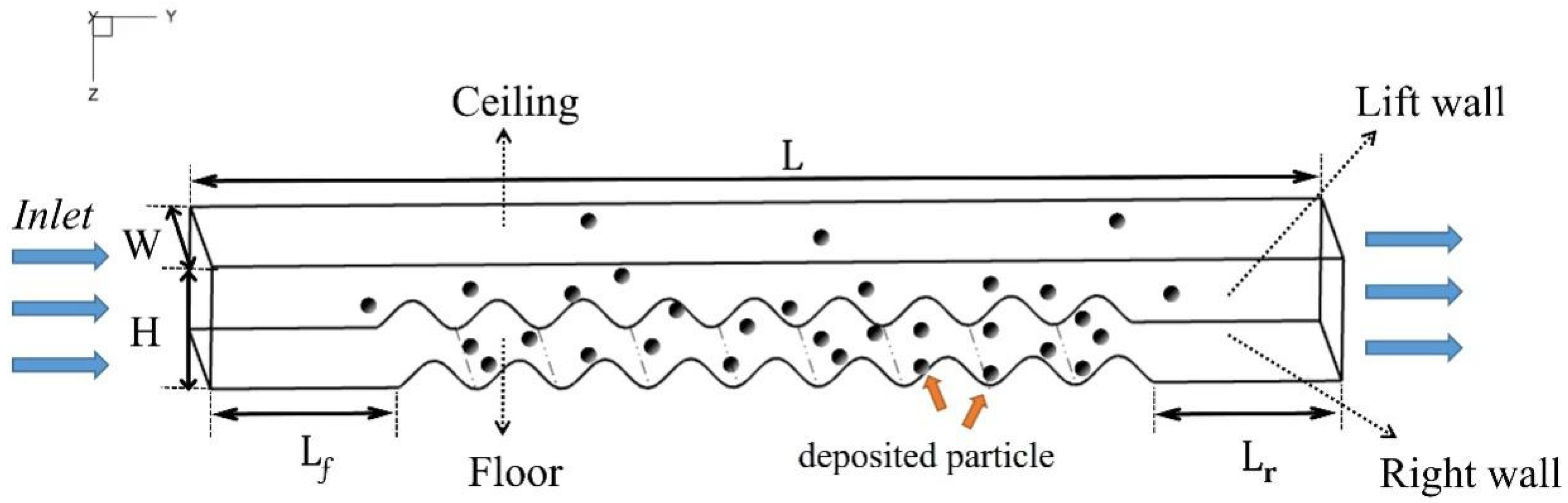
Since the actual ventilation ducts were mostly rectangular sections, this study adopted a rectangular section to study the 3D ventilation ducts. A schematic diagram of the experiment is shown in Figure 1. To reduce the influence of backflow, the front and rear ends of the corrugated section were lengthened, that is, = = 150 mm. The parameters of each part of the geometric model are shown in Table 1. According to Table 2, a total of nine cases were simulated for the study.
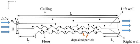
Figure 1.
Deposition of particles on a three-dimensional corrugated wall.

Table 1.
Parameters of each part.
Table 2.
Computational cases.
The contour of the corrugated wall was generated by the following expression:
3.1. Solution Method
The fluid control problem was solved using the FVM. The discrete method was employed using second-order upwind. SIMPLE was used for the calculations. A UDF was used to satisfy the requirement of full air development and to implement the particle deposition model.
3.2. Computational Grid and Grid Independence Study
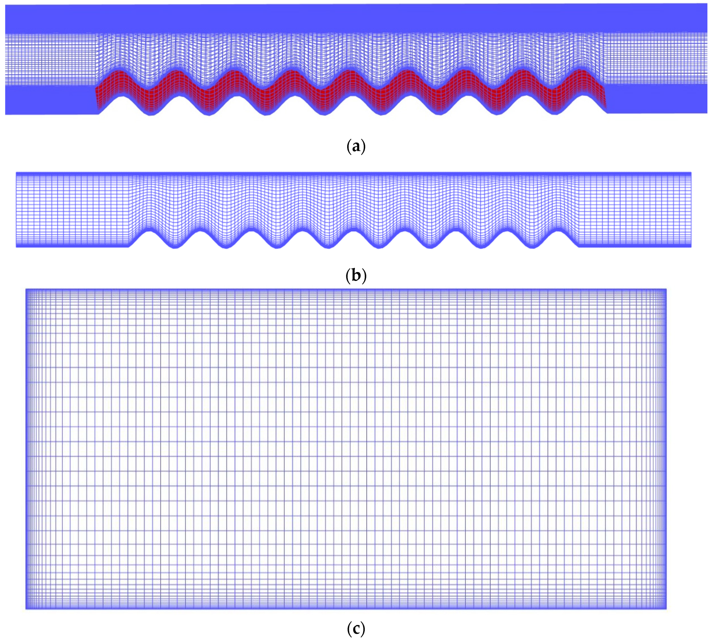
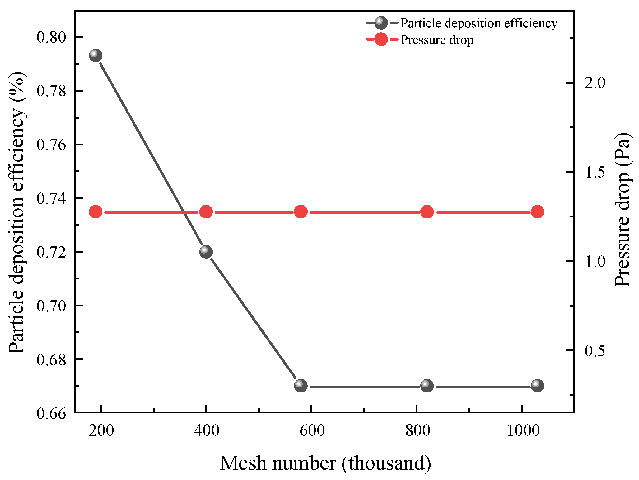
Structured meshes were generated using the commercial software ICEM. These are generally hexahedral grids, which require less computing memory, and the grids are relatively neat and close to the actual model. Therefore, this paper used a structured grid for mesh division. Additionally, mesh encryption was performed on the corrugated wall surface. Figure 2 depicts a typical organized grid system utilized in the pipelines. The first layer grid requires ≈ 1 and a growth rate of 1.1. To reduce the influence of the grid on the results, five sets of grids were used to verify the independence of the grid. The specific verification situation is shown in Figure 3. From 190,000 to 1,200,000, five grid numbers were employed in the calculation. The sensitivity of the grid was examined by using the pipe pressure drop and the deposition efficiency of 3 μm particles, and a grid of 820,000 was finally determined as the grid to be used in this study.
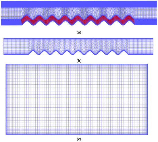
Figure 2.
Computational grid. (a) Corrugated wall pipe mesh. (b) YZ plane. (c) XZ plane.
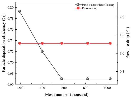
Figure 3.
Computational grid sensitivity check.
4. Results and Analysis
4.1. Results Verification
4.1.1. Verification of the Turbulent Flow Field
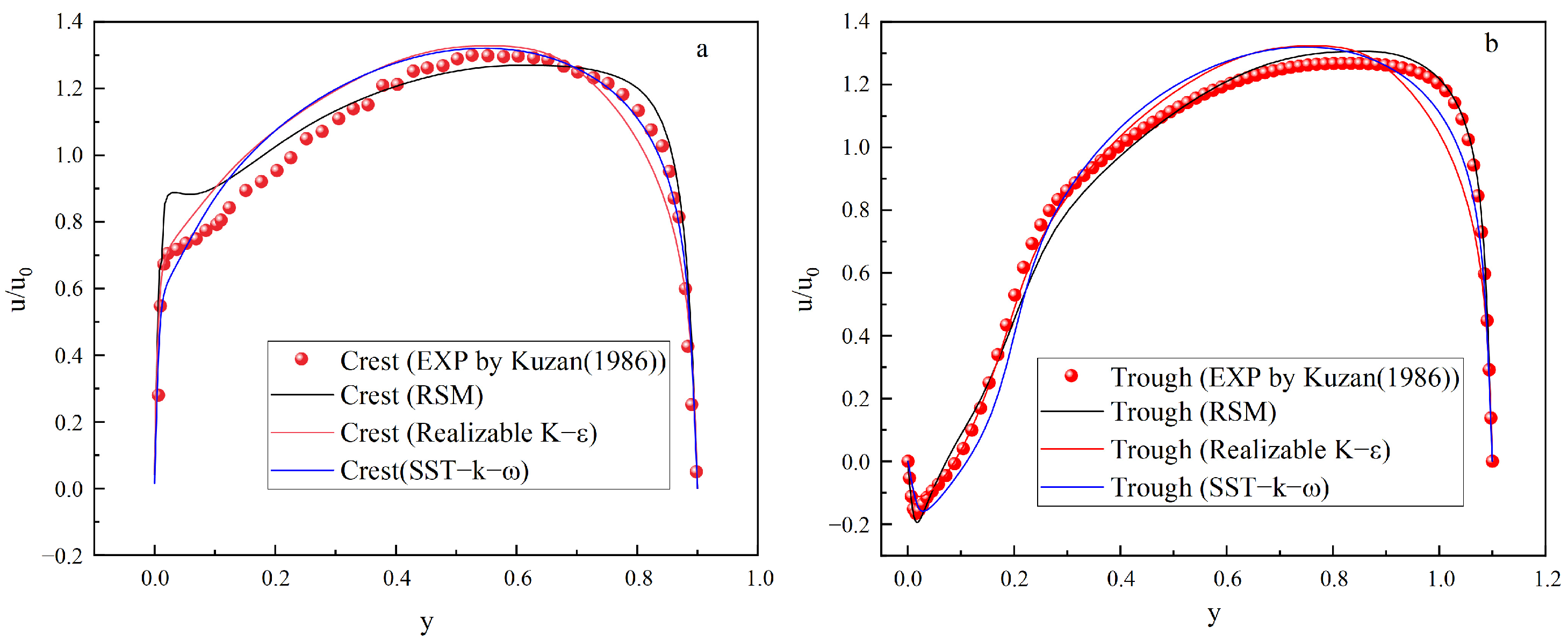
DNS data were used to ensure the accuracy of this study, and the velocity distribution in the smooth pipe was compared with that in the study of Kim et al. [52], as shown in Figure 4. In addition, the realizable k-ε model, the SST-k-ω model, and the RSM were used, and the velocity distributions at the crest and trough of the bellows were compared with Kuzan’s [53] experiments, as shown in Figure 5. The RSM model was found to be closer to the experimental results. The same conclusion was obtained by Han et al. [42] in their study. Therefore, the accuracy of the results obtained using the RSM model was better guaranteed.
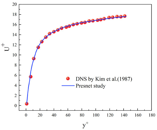
Figure 4.
Validation of turbulent flow velocity profiles using mathematics [52].

Figure 5.
Corrugated pipe speed verification. (a) Speed of crest. (b) Speed of trough [53].
4.1.2. Verification of Particle Deposition
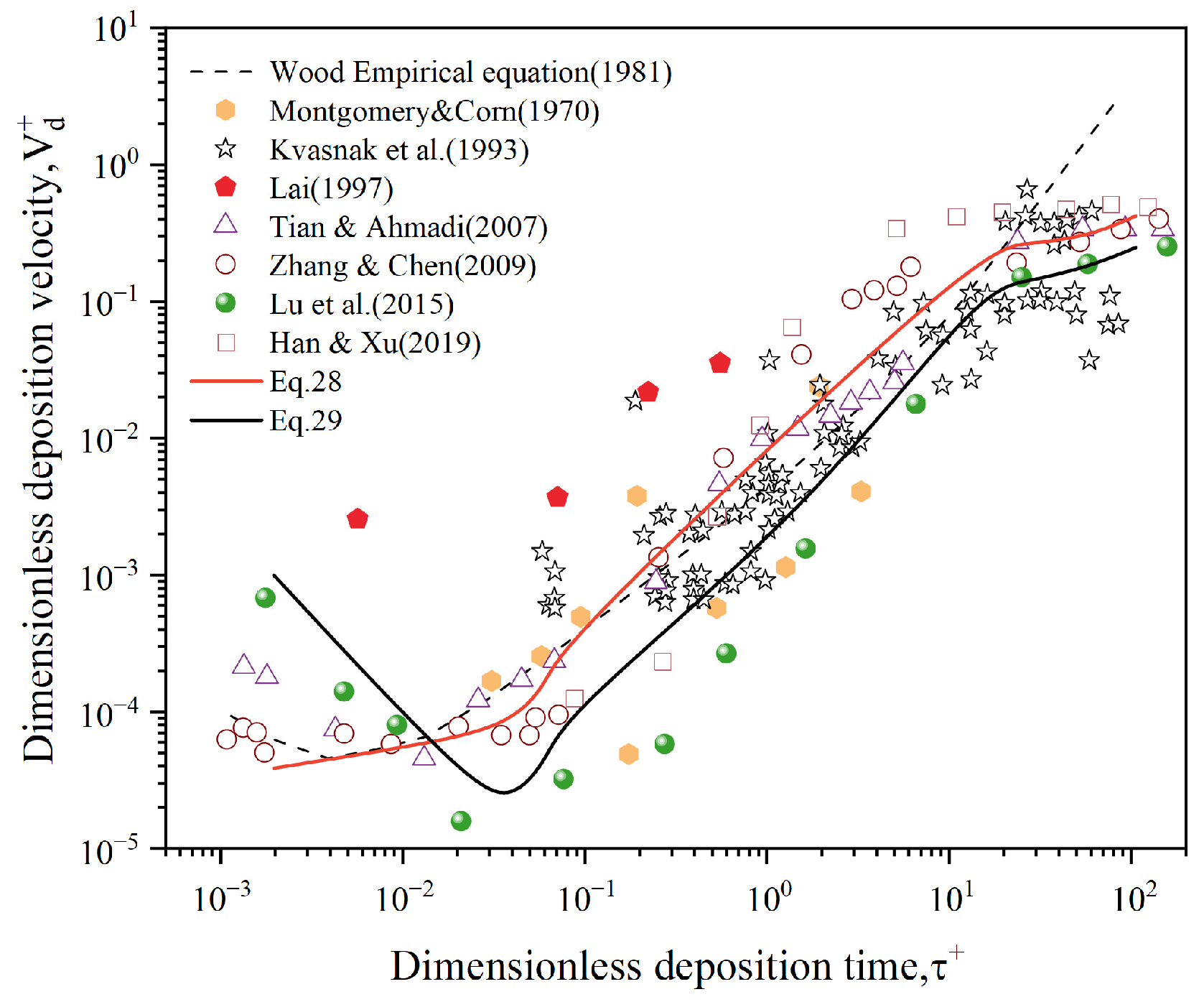
Figure 6 shows the variation in the dimensionless deposition rate of colloidal particles in smooth horizontal channels with dimensionless deposition time and compares it with the results of Wood [54] as well as other studies [3,39,42,55,56]. Comparing Equations (15) and (16), it was found that the results of Equation (15) have less error with Wood’s empirical formula. Equation (16) exhibits a distinct “V” shape, which is consistent with the results of Tian and Ahmadi et al. [3]. This is because when the particle size is small, the particles are more influenced by the flow field, and the movement of large particles is mainly influenced by inertia forces. Therefore, the particle deposition velocity decreases first and then increases.
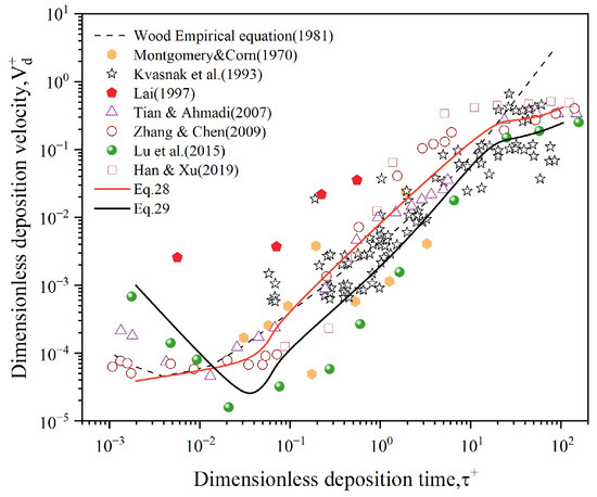
Figure 6.
Particle deposition in horizontal smooth pipes [3,6,39,42,54,55,56].
4.2. Effect of Air Velocity on the Flow Field
4.2.1. Effect of Air Velocity on Turbulence
In addition to Re, the impact of air velocity on turbulence can also be described in terms of turbulent kinetic energy (TKE). TKE is a measure of turbulence strength, and the larger the TKE, the larger the pulsation scale and the more affected is the particle motion trajectory. A cloud diagram of TKEs corresponding to different air speeds is shown in the Figure 7. The larger areas of TKE are distributed at the crest and windward side of the corrugation. As the velocity increases, the TKE also increases gradually, and along the flow direction, the largest clouds of TKE gradually increase, which indicates that in the front part of the flow field, the areas with high turbulent kinetic energy at the crest of the ripple are small, while the areas with high turbulent kinetic energy in the back part are larger and more particles will be obtained to be deposited in these areas.
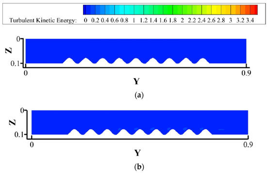
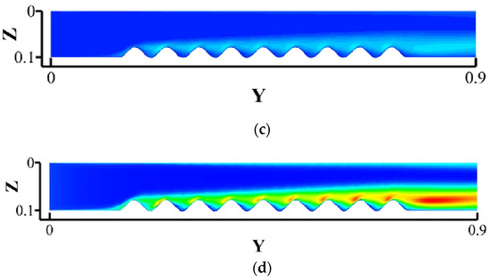
Figure 7.
Cloud images of turbulent kinetic energy (TKE) at different velocities at X = 100 mm section. (a) = 0.6 m/s. (b) = 1.6 m/s. (c) = 3.0 m/s. (d) = 7.0 m/s.
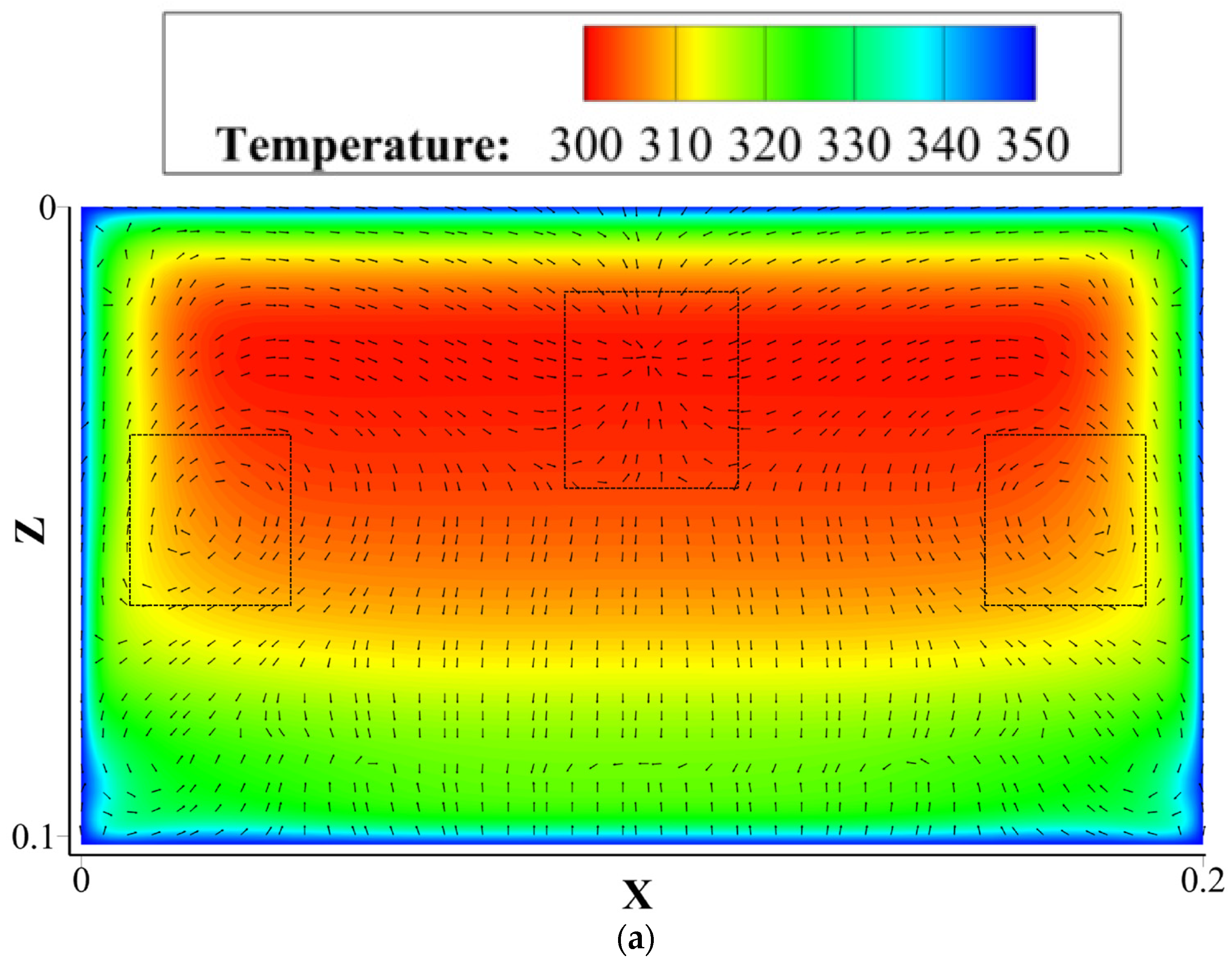
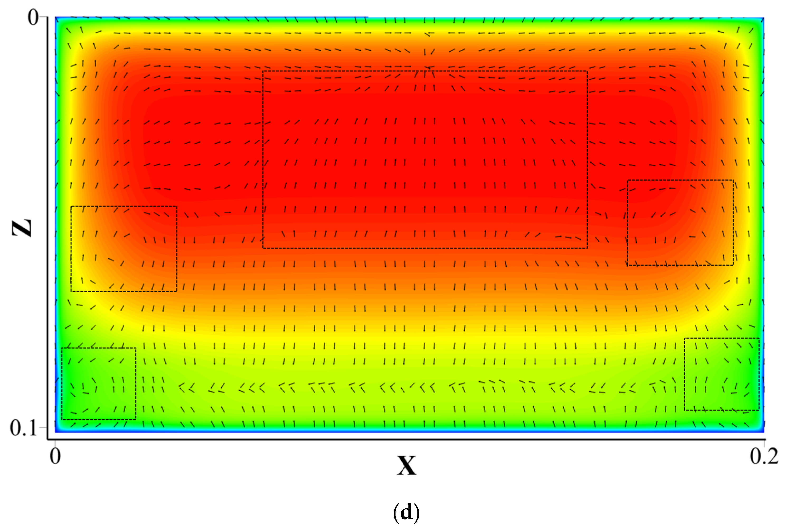
The use of corrugated walls will affect the temperature distribution in a pipe, causing a change in the temperature gradient at the wall. As the speed increases, the temperature gradient from the low-temperature center region to the corrugated wall surface gradually increases. The particles are subjected to thermophoretic force from the corrugated wall surface to the upper wall surface because the force is in the opposite direction to the temperature gradient. And the increase in velocity makes the secondary flow from the bottom of the pipe to the upper wall increase, which will make the particles be rolled and sucked away from the corrugated wall surface. The specific temperature distribution and secondary flow can be seen in Figure 8.
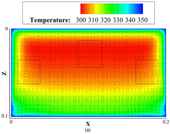
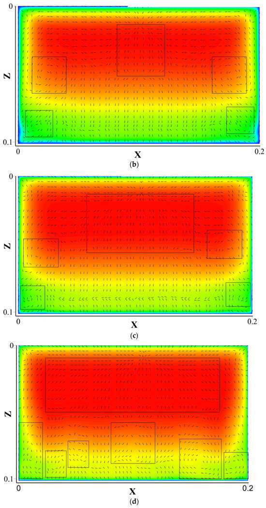
Figure 8.
Temperature cloud image and flow field vector diagram of Y = 550 mm section at different velocities. (a) = 0.6 m/s. (b) = 1.6 m/s. (c) = 3.0 m/s. (d) = 7.0 m/s.
4.2.2. Vortex Identification and Analysis
Typically, vortices are employed to quantify the rotating motion of a flow. Analysis of the impact of the flow field on particle deposition is facilitated by precise identification of the position and size of vortices. Setting a threshold value is necessary for the second-generation vortex identification method, and different threshold values have various vortex shapes. The influence of the threshold value on vortex structure can be resolved using the third-generation vortex identification method. In order to catch vortex clusters, a threshold value of 0.52 is used, and more flimsy vortex structures can be seen [57]. The specific formula is described as follows:
where, respectively, A and B represent the symmetric and antisymmetric components of the velocity gradient tensor (ΔV), while ΔV is:
A and B are calculated as follows:
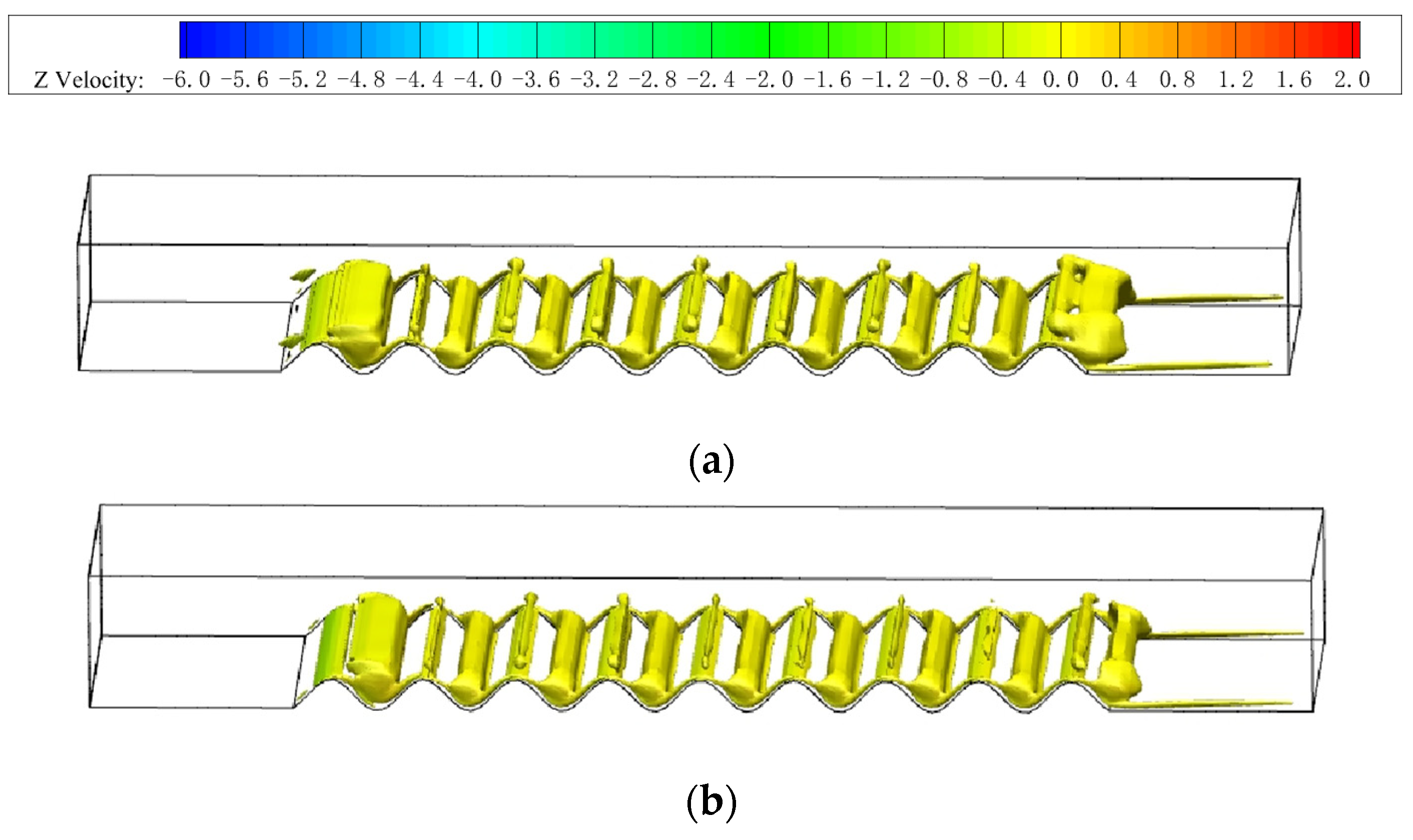
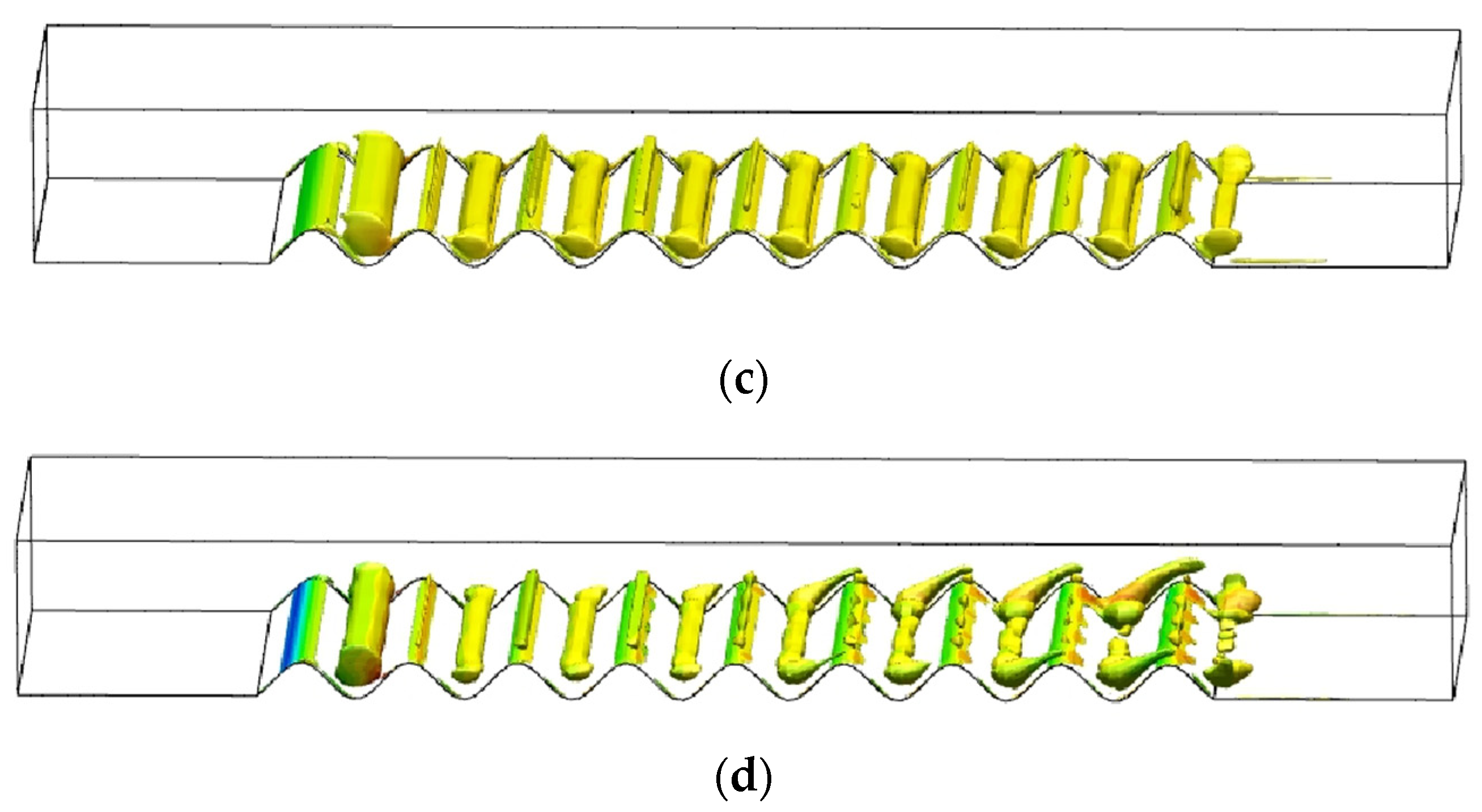
The vortex clusters are depicted in Figure 9 at various speeds. The ripple period was 6.5 mm, and the height of the ripple was 12 mm. Periodically, vortices can be seen at the peaks and valleys of the waves. The effectiveness of particle deposition on the corrugated wall will be impacted by the obvious differences in the vortex clusters on the two sides of the wall caused by the change in air velocity. As the speed increases, the size of the vortex cluster in the tank gradually decreases, which will make the ability of the vortex cluster to wind up the particles decrease, thus reducing the particle deposition efficiency. The presence of ripples causes the vortex cluster to gather particles, which greatly increases the effectiveness of particle deposition.


Figure 9.
Distribution of vortex clusters at different velocities. (a) = 0.6 m/s. (b) = 1.6 m/s. (c) = 3.0 m/s. (d) = 7.0 m/s.
The vortex cluster distribution in Figure 9d differs significantly from the other graphs in that there is an upward winding vortex cluster, and the upward velocity gradually increases with the increase in the inlet velocity, which becomes a resistance to particle deposition and thus will make the particle deposition efficiency decrease.
4.3. Effect of Different Walls on the Flow Field
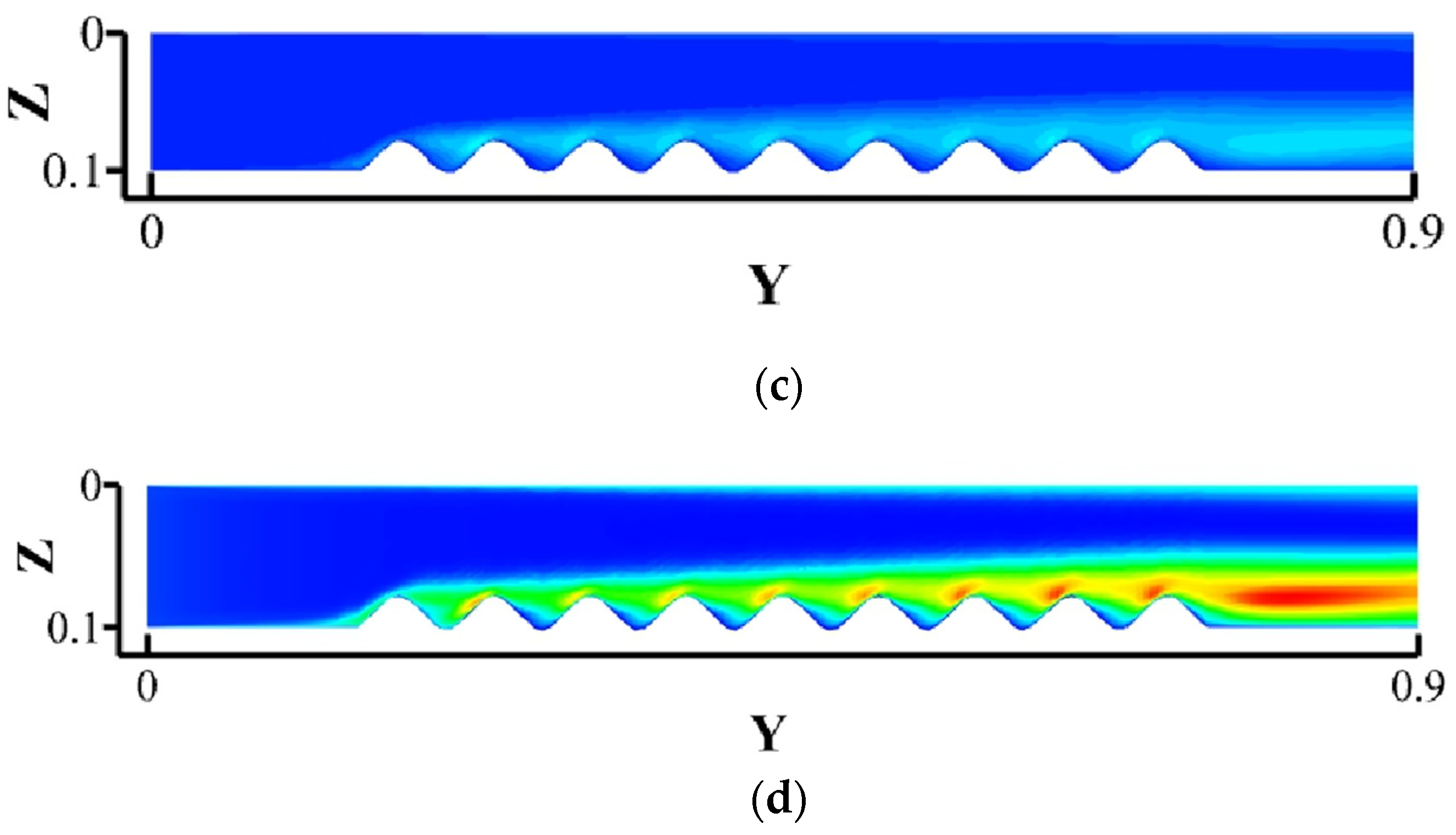
The TKE distribution in the YZ direction for different rough walls is shown in Figure 10, and the maximum value of TKE increases gradually as the height of the rough wall increases. This also proves the accuracy of this study. The TKE maximum is distributed at the pipe wall in a smooth pipe, and when a corrugated wall surface is employed in the pipe, the TKE maximum emerges at the corrugated wall surface, which can increase fluid disturbance and particle deposition. As the corrugation height increases, the area with high TKE values gradually increases and the perturbation of the whole flow field becomes more intense. In addition, there is a clear boundary layer at the smooth tube wall surface, and the boundary layer is destroyed at the tube wall after using the corrugated wall surface, which will increase the heat transfer efficiency.
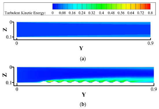
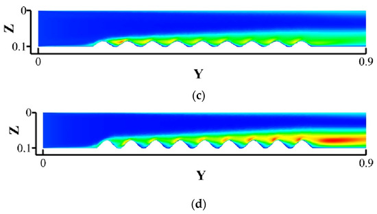
Figure 10.
Cloud plot of turbulent kinetic energy (TKE) for different rough wall surfaces at X = 100 mm section. (a) Smooth. (b) Corrugated wall height (h) = 5 mm. (c) Corrugated wall height (h) = 8 mm. (d) Corrugated wall height (h) = 12 mm.
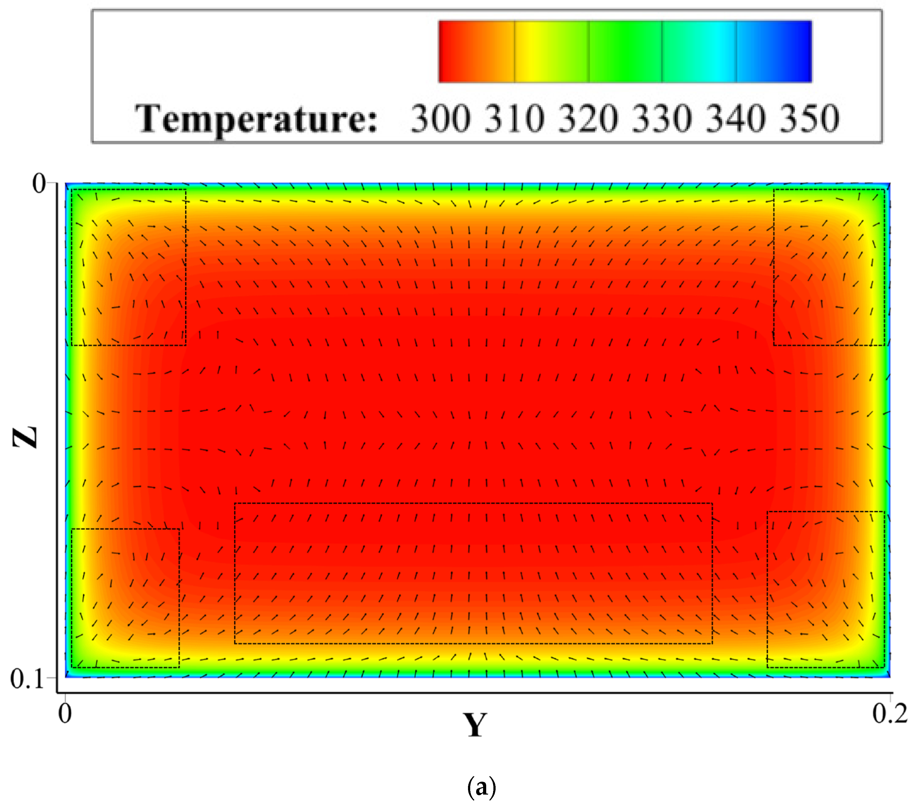
Figure 11 shows the temperature clouds and velocity vector plots under walls of different roughnesses, where the temperature distribution is relatively uniform in the smooth channel. As the corrugation height increases, the temperature center is shifted upward, making the distance from the rough wall to the temperature center of the pipe increase, which results in a lower temperature gradient and a lower thermal swimming force. Vortex clusters exist in all four corners of the smooth pipe, and in the part near the bottom, an upward flow field exists, while a downward flow field will exist at the bottom with the corrugated wall surface. The deposition of small particles is influenced by the flow field, so the corrugated wall surface will enhance the deposition efficiency of small particles. As the ripple height increases, the flow field in the bottom region becomes more turbulent. The vortex cluster area also gradually increases, which will increase the deposition efficiency of small particles.
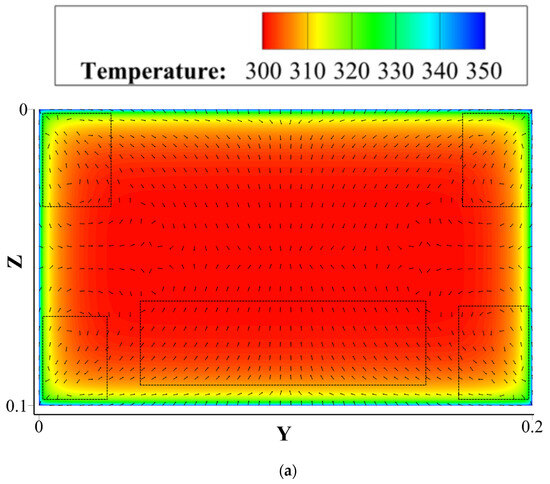
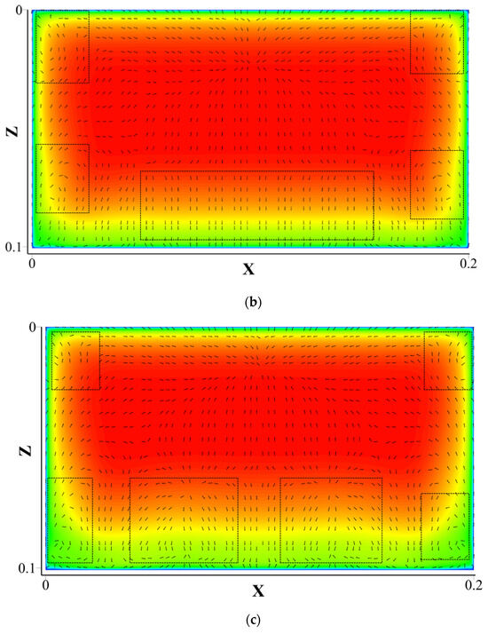
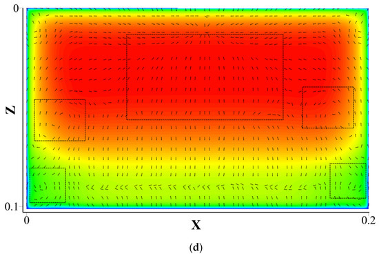
Figure 11.
Temperature cloud image and flow field vector diagram of Y = 550 mm section at X = 100 mm section. (a) Smooth. (b) Corrugated wall height (h) = 5 mm. (c) Corrugated wall height (h) = 8 mm. (d) Corrugated wall height (h) = 12 mm.
4.4. Deposition Characteristics of Micron Particles
4.4.1. Effect of Rebound on Particle Deposition
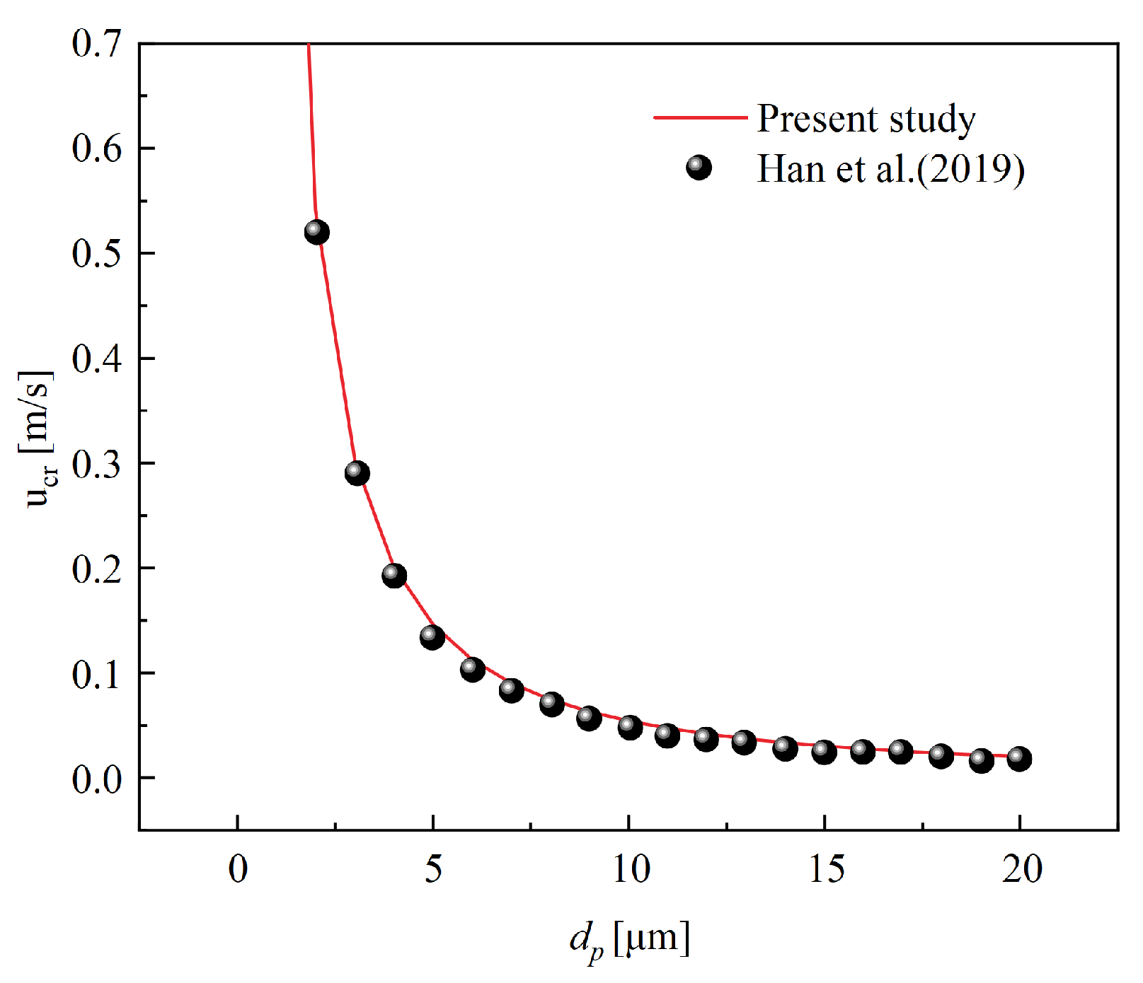
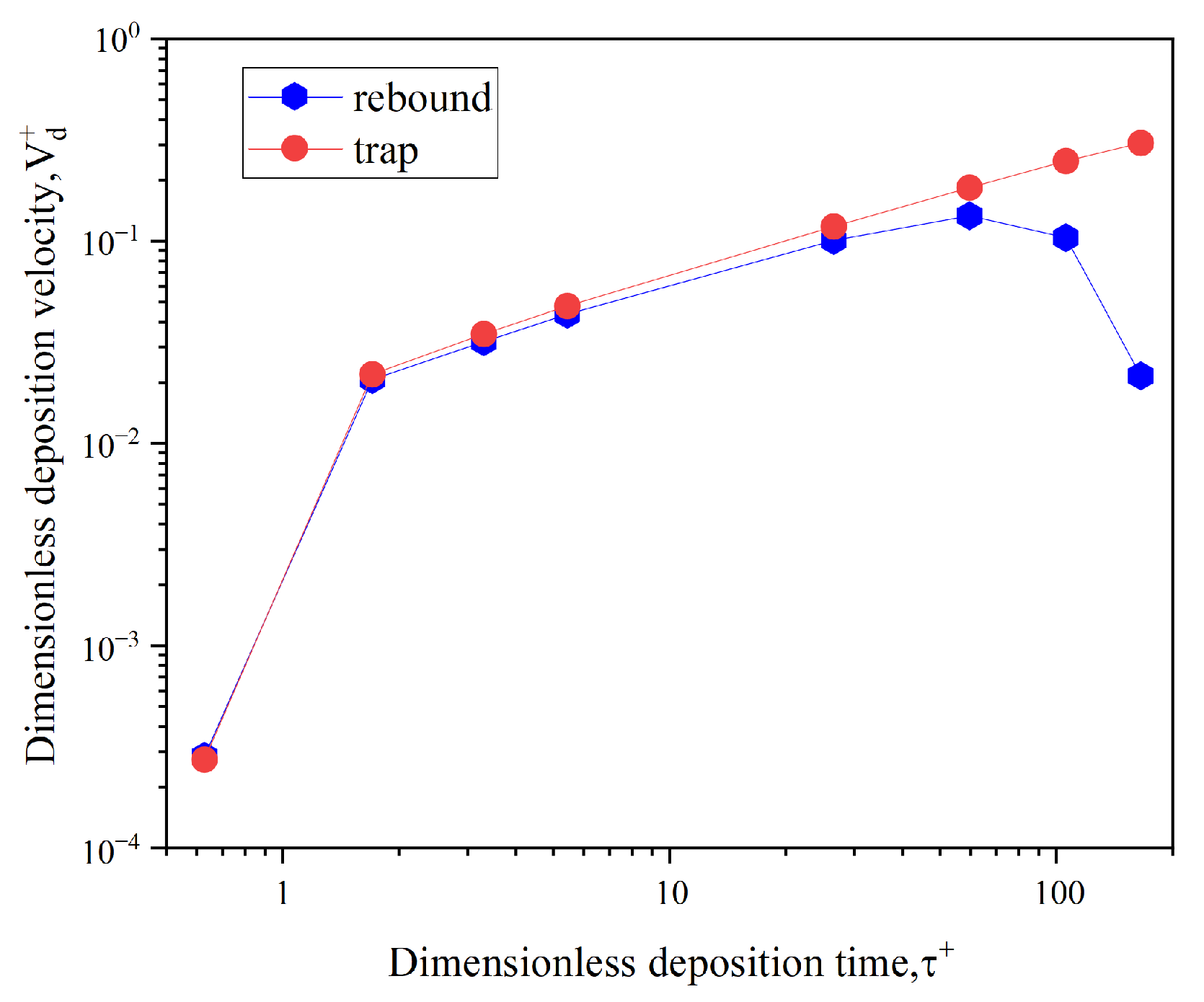
Figure 12 shows a comparison of the critical particle deposition velocities for different particle sizes with the results of Han et al. [42]. As particle size grows, the critical velocity drops. This means that larger-sized particles are more prone to rebound. Figure 13 compares the two different deposition models and shows that small particles are less affected by bounce while large particles are more affected by bounce, along with the deposition rate decreases for larger particle sizes. These were due to the higher kinetic energies of the larger particles and the smaller critical velocities. The same results were obtained by Sun et al. [44].
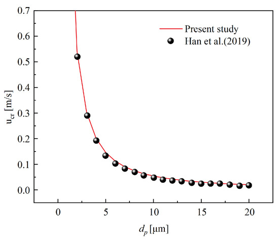
Figure 12.
Verification of the critical velocity of particle bounce [42].

Figure 13.
Effect of rebound on particle dimensionless deposition rate.
4.4.2. Effect of Air Velocity on Particle Deposition
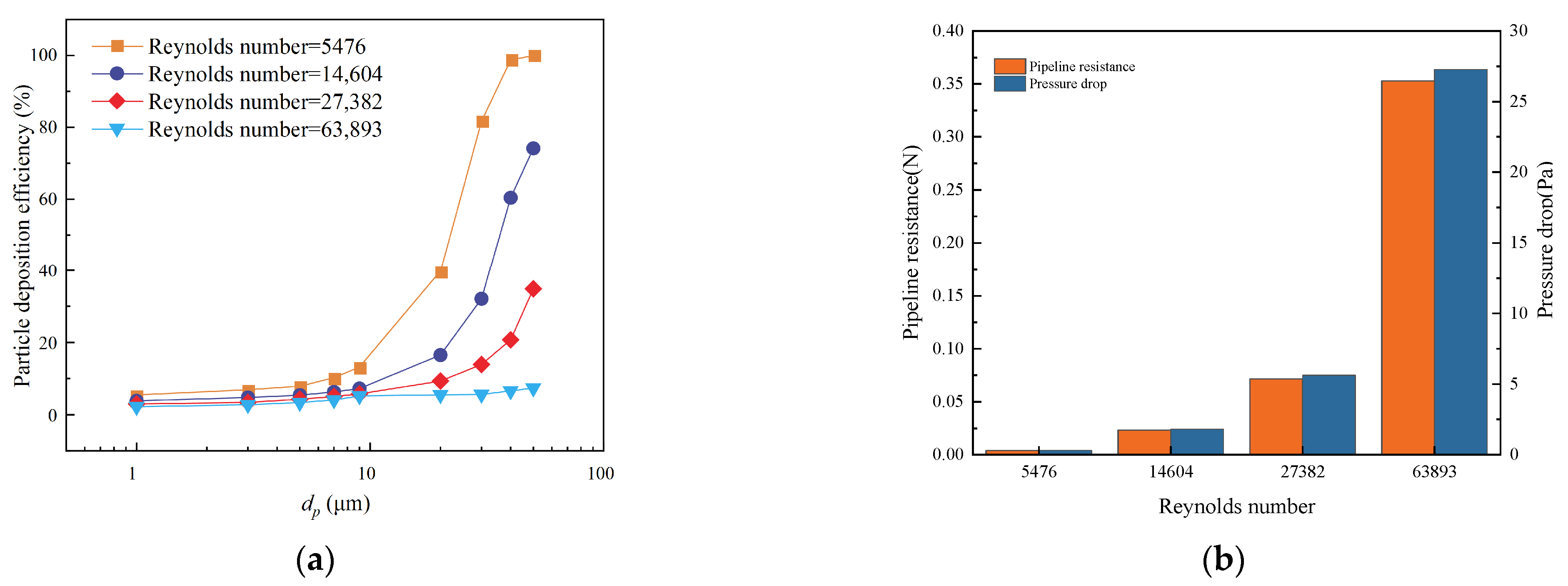
Figure 14 shows the values at different air velocities and that decreases with the increase in air velocity. At lower air velocities, gradually increases with the increase in . When the is high, varies less with . This occurs because the is high, the negative velocity in the z-axis direction also gradually increases, and the deposition of large particles mainly relies on gravitational sedimentation, so that the of large particles decreases. As the increases, the wall resistance and pipe pressure drop gradually increase. Therefore, different simultaneous smaller particle depositions and smaller pressure drops were obtained.
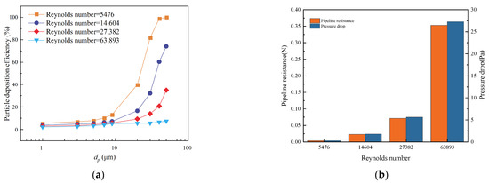
Figure 14.
Particle deposition efficiency and pipe pressure drop and resistance at different speeds. (a) Particle deposition efficiency. (b) Pipe pressure drop and resistance.
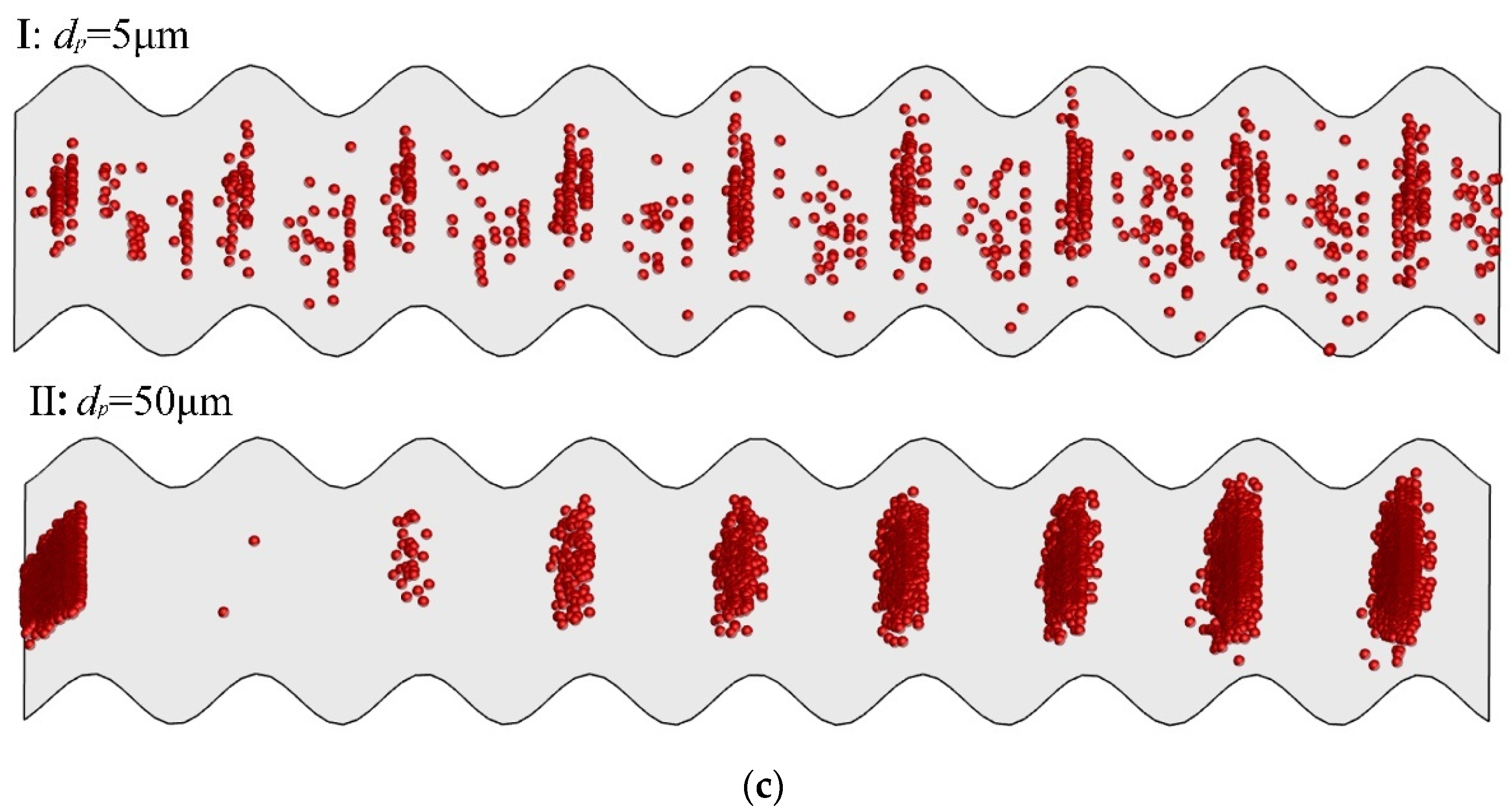
Figure 15 shows the position of particle deposition for two different particle sizes (5 μm and 50 μm) with different air velocities. When dp = 5 μm, the number of particles deposited in the latter part of the corrugated wall was higher than that in the former part, and the deposition was concentrated in the crest and trough of the corrugation, with the deposition at the crest being arranged in a straight line. As the dp became larger, the deposition position changed more, and when the air velocity was small, more particles of 50 μm were deposited in the front part of the corrugation. Particles were gradually deposited at the back of the corrugated wall with an increase in air velocity. In addition, large particles were deposited more at the entrance. When the air velocity was 7 m/s, 50 μm particles were deposited at the front and rear ends of the corrugation and less at the center part of the corrugation. This is thought to be because tiny particles, which have a lower mass, can follow fluid flow more effectively. The likelihood of small particles bouncing in the front section of the corrugated wall increases as the velocity and kinetic energy of the particles increases. After a few bounces, the kinetic energy of the particles reduces on the corrugated wall surface in the back, increasing the number of particles deposited. When the velocity is low, the kinetic energy of the particles is low and they are easily deposited in the front portion of the corrugated wall. Inertial forces are the primary factors that affect the deposition of big particles. As the velocity increases, the deposition concentration area gradually moves to the rear part of the corrugated wall. Large particles have a low critical velocity; hence, increasing velocity also improves the likelihood of large particles rebounding. Therefore, under the impact of the two aforementioned parameters, the efficiency of large particle deposition rapidly declined as the velocity reached 7 m/s.
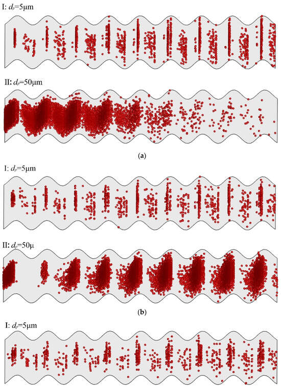

Figure 15.
Particle deposition locations for different air velocities. (a) = 0.6 m/s. (b) = 1.6 m/s. (c) = 3.0 m/s. (d) = 7.0 m/s. (I for 5 μm, II for 50 μm).
4.4.3. Effect of Corrugation Height on Particle Deposition
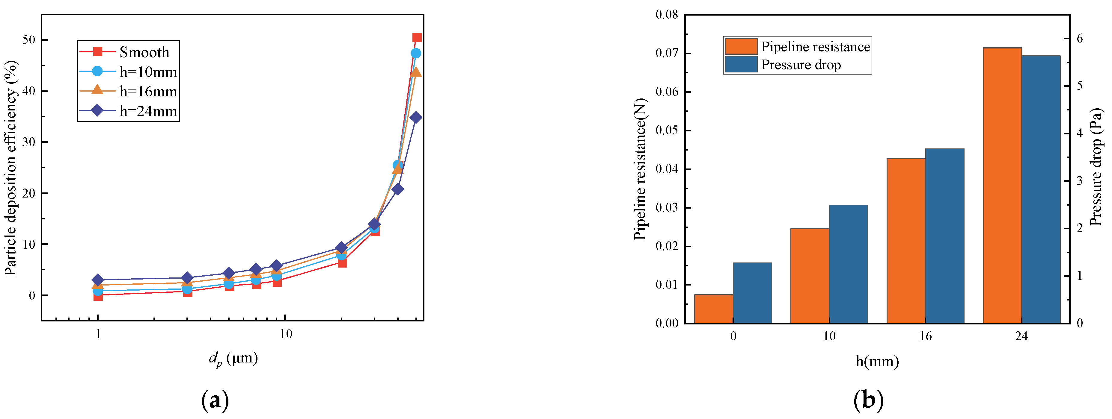
Figure 16 illustrates the particle deposition efficiency and the pipe pressure drop and pipe resistance at different rough wall heights. As the rough wall height increases, the pipeline pressure drop and pipeline resistance also increase. When dp < 30 μm, increases with the increase in pipe resistance. When dp > 30 μm, and pipe resistance show negative correlation. This is because when the corrugation height increases, the upward vortex mass gradually increases, which makes the large particles be subject to larger resistance, and thus the particle deposition efficiency decreases. Compared to the effect of air velocity variation on particle deposition, it is more costly to use increased rough wall height to achieve proper particle deposition.
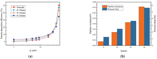
Figure 16.
Particle deposition efficiency and pipe pressure drop and resistance at different corrugation heights. (a) Particle deposition efficiency. (b) Pipe pressure drop and resistance.
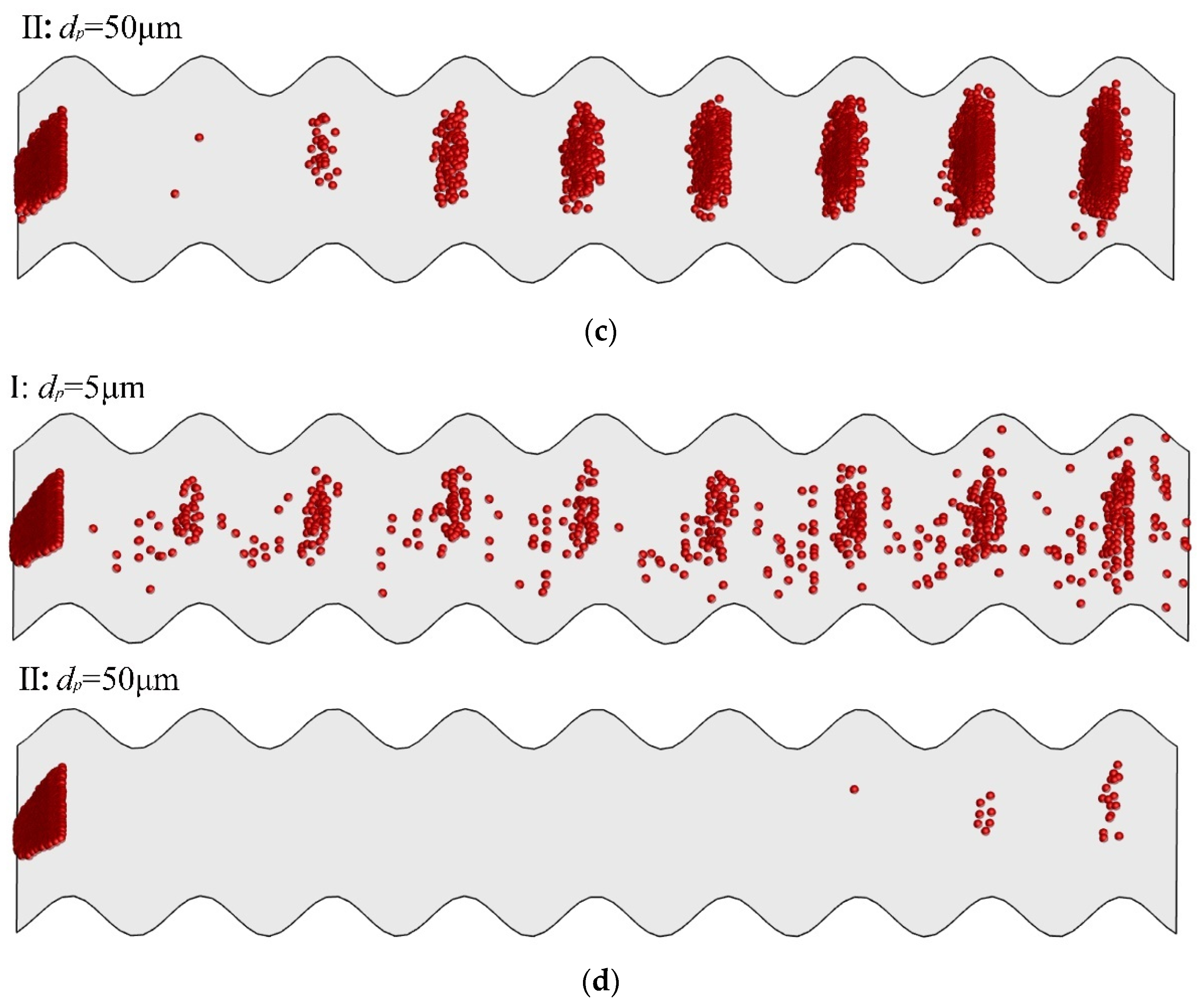
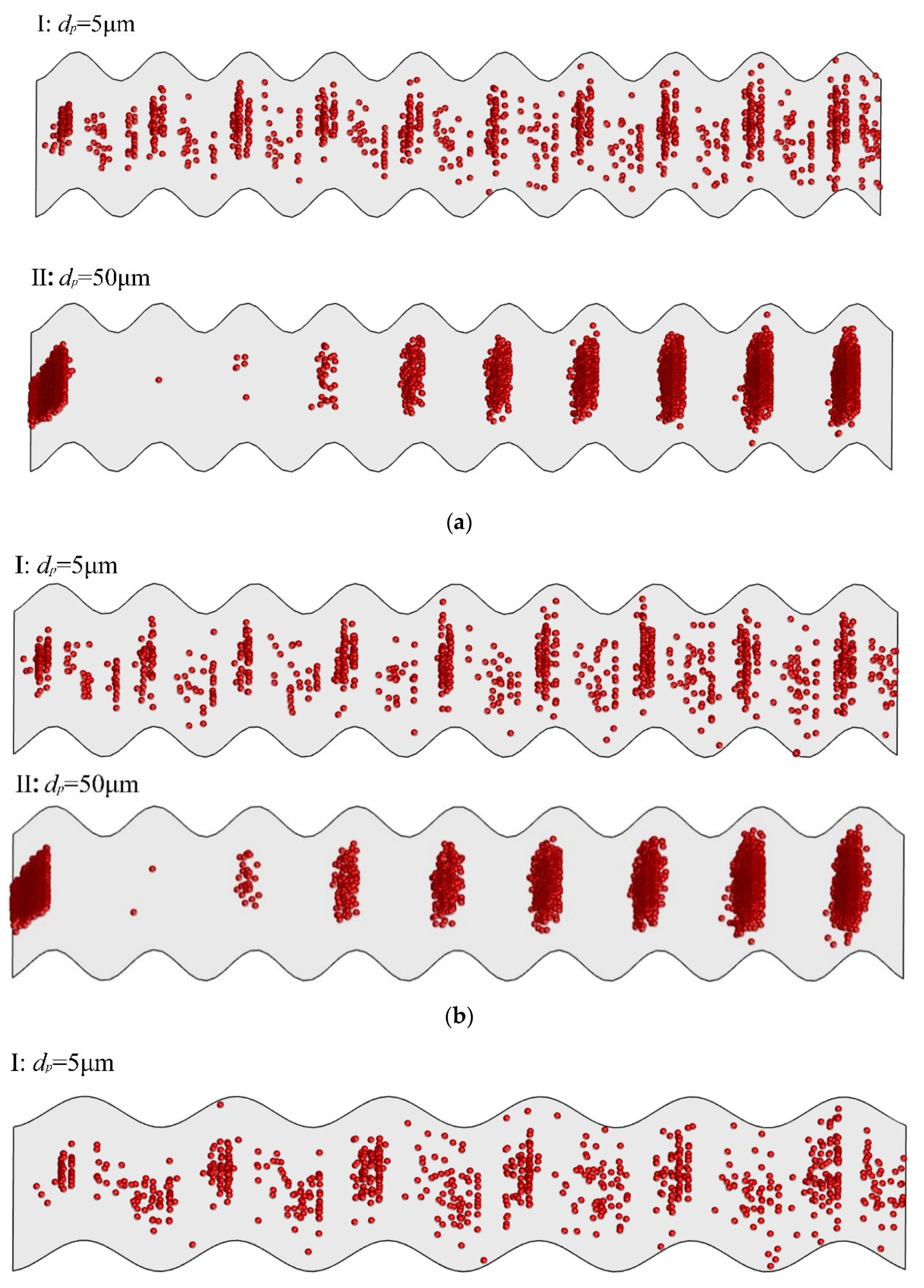
Figure 17 illustrates the effect of different ripple heights on the location of particle deposition, where I indicates a 5 μm particle and II indicates dp = 50 μm. The particles were deposited less at the entrance of the corrugation, and the number of particles deposited gradually increased along the flow square. The number of particles deposited at the corrugation inlet steadily decreased as the corrugation height rose when dp = 50 μm. The front portion of the corrugation developed a particle-free area even at a corrugation height of 24 mm. This was mainly because, as the corrugation height increased, the particles with large particle sizes had a greater chance of bouncing at the front part of the corrugation, making the particles less likely to be deposited.
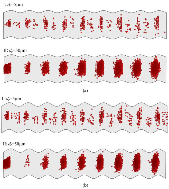

Figure 17.
Schematic representation of particle deposition locations with different ripple heights. (a) h = 10 mm. (b) h = 16 mm. (c) h = 24 mm. (I for 5 μm, II for 50 μm.)
In the case of larger particles, particle deposition is mostly focused on the windward side of the ripple and at the wave’s crest, with less deposition in the trough. This is because small particles will be deposited at the trough due to the vortex at the trough, while the main deposition mechanism of large particles is gravitational sedimentation, so it is difficult for the secondary flow at the trough to absorb large particles, while the particle impact at the crest will result in a reduction in part of the particles’ kinetic energy and thus their deposition at the crest.
4.4.4. Effect of Corrugation Period on Particle Deposition
Figure 18 illustrates the particle deposition efficiency, pressure drop, and pipe resistance for different corrugation cycles. When dp < 30 μm, the deposition efficiency gradually increased as the corrugation period decreased. When dp > 30 μm, was larger for the corrugation cycle of T = 6.5 mm, and the corrugation wall of T = 5.7 mm had a higher particle deposition efficiency than the corrugation wall of T = 9.75 mm at a particle size of 50 μm. As the cycle lengthened, the pipe’s resistance steadily reduced, which was caused by a reduction in both the number of corrugations and the perimeter of the corrugated wall surface. However, the pressure drop did not decrease with the increase in the corrugation period, and the pressure drop of the pipe was higher when the corrugation period (T) = 9.75 mm than when T = 6.5 mm.
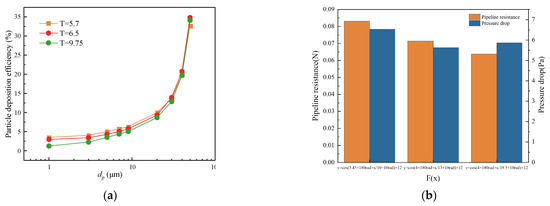
Figure 18.
Particle deposition efficiency and pipeline pressure drop and resistance at different corrugation periods. (a) Particle deposition efficiency. (b) Pipe pressure drop and resistance.
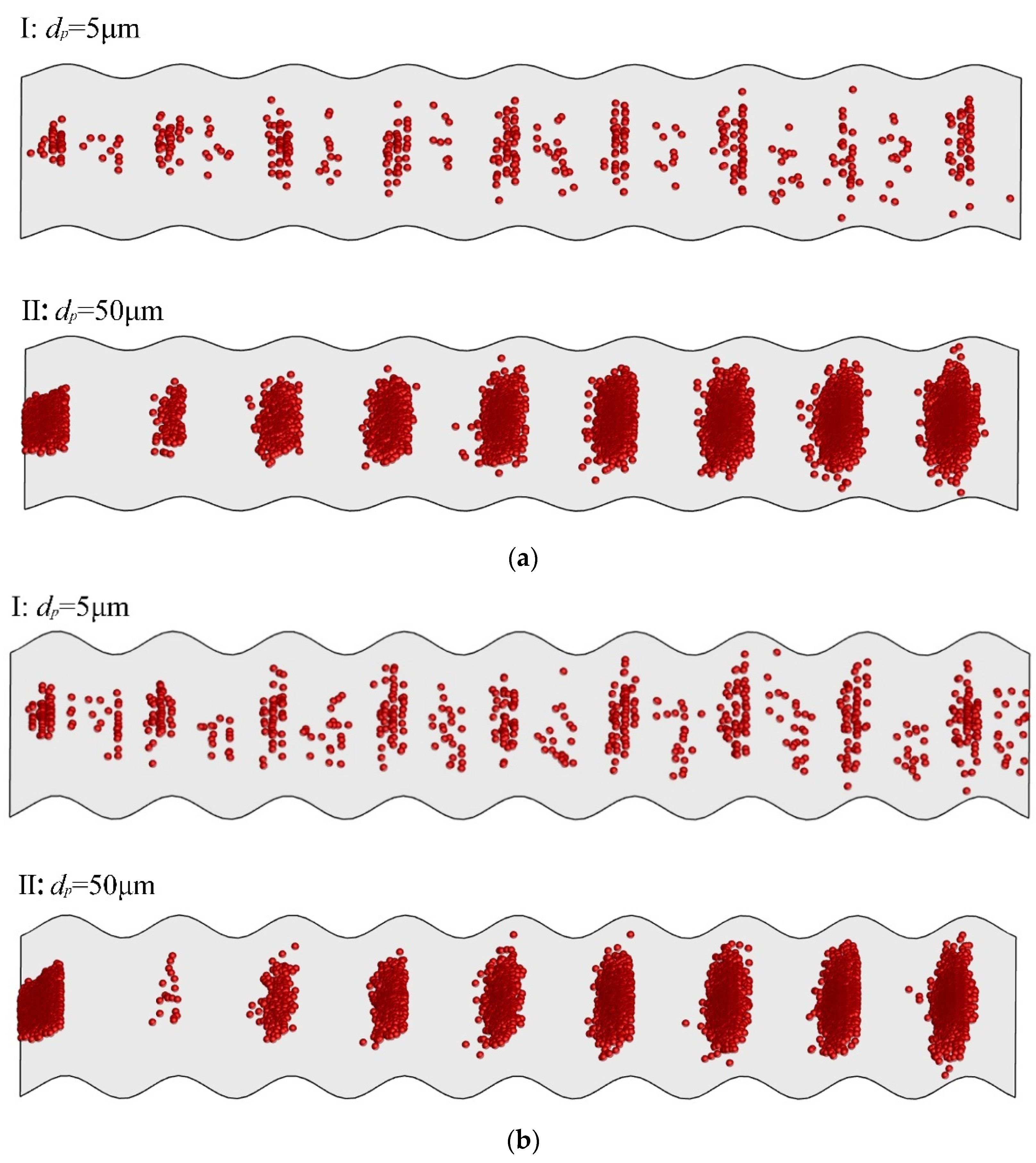
Figure 19 illustrates how the particles are deposited in each cycle of the corrugation when the period is short and the dp = 5 μm. Therefore, for corrugated plates with tiny cycles, is higher when the particle size is smaller. As dp increases, when dp = 50 μm, the particles are deposited on the corrugated plate and the aggregation of deposition along the flow square is more obvious and mainly at the crest and windward side. This makes the deposition efficiency of the corrugated plate with T = 9.75 mm higher than that of the corrugated plate with T = 5.7 mm at dp = 50 μm. Therefore, the larger the corrugated wall surface is for longer periods, the better the particle deposition at the corrugated plate.
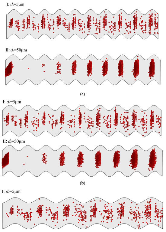
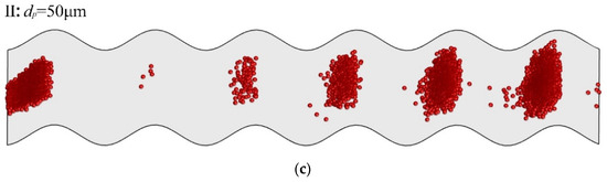
Figure 19.
Schematic diagram of particle deposition locations for different ripple periods. (a) T = 5.70 mm. (b) T = 6.50 mm. (c) T = 9.75 mm.
5. Conclusions
Corrugated walls enhance heat transfer and represent a frequently employed structure in conduits designed for heat transfer. While more research has been undertaken on heat transfer in corrugated walls, studies on particle deposition in corrugated channels featuring trigonometric image shapes are relatively scarce. To enhance our comprehension of particle deposition characteristics in a corrugated-wall ventilation channel with a trigonometric image shape, this investigation examined the impacts of varying corrugation heights, corrugation periods, particle sizes, deposition models, and wind velocities on particle deposition by coupling the RSM and the DPM. By analyzing the turbulent flow field, secondary flow, particle deposition efficiency, and particle deposition location, the following conclusions can be drawn:
- The use of corrugated walls enhances the deposition efficiency of particles with particle sizes (dp) < 30 μm, and when the particle size (dp) > 30 μm, particles are more likely to bounce off the corrugated walls, which makes the particle deposition efficiency lower than that for smooth walls. The particle deposition efficiency shows a positive correlation with particle size. When the corrugation height is 24 mm and dp = 3 μm, the particle deposition efficiency on a corrugated wall is five times higher than that on a smooth wall.
- Air velocity is an important factor affecting this study. The maximum value of TKE near the corrugated wall surface occurs periodically at the crest and windward side. The value of TKE increases gradually with increase in inlet air velocity. Therefore, more secondary flow occurs at the crest and windward side with increasing velocity, which can lead to changes in particle deposition efficiency. As the air velocity increases, the rebound probability of large-size particles (dp > 10 μm) increases, so the deposition efficiency of large-size particles decreases. Regarding particle deposition location, the air velocity has a strong influence on the deposition location of large particles; as the air velocity increases, the dense area of particle deposition will gradually move from the inlet to the outlet, and eventually only a small portion of the particles will be deposited at the inlet and outlet due to the rebound.
- The shape of the corrugated wall surface is an important factor affecting this study. With the increase in the corrugation height, the TKE value at the crest of the corrugated wall will gradually increase, and the secondary flow will gradually move upward. When dp < 30 μm, the deposition characteristics are mainly determined by the flow vortices and mass inertia, so the particle deposition efficiency will gradually increase with the increase in the corrugation height. The particle deposition efficiency gradually increases with the decrease in the ripple period, and particles are deposited in every ripple period. At dp > 30 μm, the particle deposition efficiency is inversely correlated with the ripple height due to rebound. The particle deposition efficiency does not gradually increase with the decrease in the corrugation period. In this study, the highest particle deposition efficiency was observed for the corrugated plate with T = 6.5 mm, and with the increase in the corrugation period, a particle-free region appeared in the front section of the corrugated wall.
Author Contributions
Conceptualization, H.L. (Hongchang Li) and H.L. (Hao Lu); methodology, Y.W.; software, Y.W.; validation, Y.W., H.L. (Hao Lu) and H.L. (Hongchang Li); investigation, H.L. (Hao Lu); resources, H.L. (Hongchang Li); data curation, Y.W. and W.Z.; writing—original draft preparation, Y.W.; writing—review and editing, H.L. (Hao Lu) and W.Z.; supervision, H.L. (Hongchang Li); project administration, H.L. (Hongchang Li); funding acquisition, H.L. (Hao Lu) All authors have read and agreed to the published version of the manuscript.
Funding
The authors appreciate the financial support provided by the National Oversea High-level Talents Program of China, National Natural Science Foundation of China (no. 52266017), and the Major Project of the National Social Science Foundation of China (no. 21&ZD133). The study was also supported by the Xinjiang Natural Science Fund for Distinguished Young Scholars (no. 2021D01E08), the Xinjiang Regional Coordination Special Project—International Science and Technology Cooperation Program (no. 2022E01026), the Xinjiang Major Science and Technology Special Project (nos. 2022401002-2, 2022A01007-1, 2022A01007-4), the Xinjiang Key Research and Development Project (nos. 2022B03028-2, 2022B01033-2, 2022B01022-1), the Central Guidance on Local Science and Technology Development Project (no. ZYYD2022C16), the Innovation Team Project of Xinjiang University (no. 500122006021), and the High-level Talents Project of Xinjiang University (no. 100521001).
Data Availability Statement
The data that support the findings of this study are available from the corresponding author upon reasonable request.
Conflicts of Interest
The authors declare no conflicts of interest.
Nomenclature
| A | Pipe section area, m2 |
| A | Symmetric component of the velocity gradient tensor |
| B | Antisymmetric component of the gradient tensor |
| Drag coefficient of particle | |
| dp | Particle diameter, μm |
| Hydraulic diameter | |
| Young’s modulus of channel wall, GPa | |
| Young’s modulus of particle, GPa | |
| Fanning friction factor | |
| Drag force, N | |
| Gravity and buoyancy, N | |
| Brownian force, N | |
| Saffman lift, N | |
| Thermophoretic force, N | |
| Gravitational acceleration, m/s2 | |
| H | Pipe height, m |
| h | Corrugated wall height, mm |
| Number of particles deposited per unit time and unit area | |
| Turbulent kinetic energy (TKE), m2·s−1 | |
| Effective stiffness parameter | |
| Average roughness height | |
| Deposited particle number | |
| Released particle number | |
| Time-averaged pressure, Pa | |
| R | Kinematic restitution coefficient |
| Reynolds number | |
| S | The particle-to-fluid density ratio |
| The maximum deposition time of particles | |
| Inlet temperature, K | |
| Wall temperature, K | |
| Critical deposition velocity | |
| Friction velocity | |
| The component of the time-averaged velocity | |
| Mean flue gas velocity, m/s | |
| Particle deposition velocity | |
| Dimensionless particle deposition velocity | |
| Dimensionless distance from the wall | |
| Greek symbols | |
| Dissipation rate of turbulent kinetic energy | |
| Nondimensional particle relaxation time | |
| Kinematic viscosity | |
| Poisson’s ratio of the wall | |
| Poisson’s ratio of the particle | |
| Particle deposition efficiency | |
| Density, kg/m3 |
Abbreviation
| RSM | Reynolds stress model |
| DPM | Discrete particle model |
| UDF | User-defined function |
| HVAC | Heating, ventilation and air conditioning |
| IAQ | Indoor air quality |
| GFEM | Galerkin finite-element method |
| CCD | Central composite design |
| FVM | Finite volume method |
| RANS | Reynolds-averaged Navier–Stokes |
| DNS | Direct numerical simulation |
| LES | Large eddy simulation |
| LBM | Lattice Boltzmann method |
| EWF | Enhanced wall function |
| TKE | Turbulent kinetic energy |
References
- Dockery, D.W.; Stone, P.H. Cardiovascular risks from fine particulate air pollution. N. Engl. J. Med. 2007, 356, 511–513. [Google Scholar] [CrossRef] [PubMed]
- Marval, J.; Tronville, P. Ultrafine particles: A review about their health effects, presence, generation, and measurement in indoor environments. Build. Environ. 2022, 216, 108992. [Google Scholar] [CrossRef]
- Tian, L.; Ahmadi, G. Particle deposition in turbulent duct flows—Comparisons of different model predictions. J. Aerosol Sci. 2007, 38, 377–397. [Google Scholar] [CrossRef]
- Othmane, M.B.; Havet, M.; Gehin, E.; Solliec, C. Mechanisms of Particle Deposition in Ventilation Ducts for a Food Factory. Aerosol Sci. Technol. 2010, 44, 775–784. [Google Scholar] [CrossRef]
- Dehbi, A. A CFD model for particle dispersion in turbulent boundary layer flows. Nucl. Eng. Des. 2008, 238, 707–715. [Google Scholar] [CrossRef]
- Lai, A.C.; Byrne, M.A.; Goddard, A.J. Aerosol deposition in turbulent channel flow on a regular array of three-dimensional roughness elements. J. Aerosol Sci. 2001, 32, 121–137. [Google Scholar] [CrossRef]
- Lai, A.C.; Byrne, M.A.; Goddard, A.J. Particle deposition in ventilation duct onto three-dimensional roughness elements. Build. Environ. 2002, 37, 939–945. [Google Scholar] [CrossRef]
- Lu, H.; Lu, L. A numerical study of particle deposition in ribbed duct flow with different rib shapes. Build. Environ. 2015, 94, 43–53. [Google Scholar] [CrossRef]
- Lu, H.; Quan, Y. A CFD study of particle deposition in three-dimensional heat exchange channel based on an improved deposition model. Int. J. Heat Mass Transf. 2021, 178, 121633. [Google Scholar] [CrossRef]
- Bi, C.; Tang, G.H.; Tao, W.Q. Heat transfer enhancement in mini-channel heat sinks with dimples and cylindrical grooves. Appl. Therm. Eng. 2013, 55, 121–132. [Google Scholar] [CrossRef]
- Han, Z.; Lu, H. Numerical simulation of turbulent flow and particle deposition in heat transfer channels with concave dimples. Appl. Therm. Eng. 2023, 230, 120672. [Google Scholar] [CrossRef]
- Kooh Andaz, A.; Dal Maso, M. Effect of a deflector on deposition of particles with different diameters in a rib-roughened channel. Powder Technol. 2023, 428, 118831. [Google Scholar] [CrossRef]
- Launder, B.E.; Reece, G.J.; Rodi, W. Progress in the development of a Reynolds-stress turbulence closure. J. Fluid Mech. 1975, 68, 537–566. [Google Scholar] [CrossRef]
- Hamida, M.B.B.; Almeshaal, M.A.; Hajlaoui, K.; Rothan, Y.A. A three-dimensional thermal management study for cooling a square Light Edding Diode. Case Stud. Therm. Eng. 2021, 27, 101223. [Google Scholar] [CrossRef]
- Hamida, M.B.B.; Hatami, M. Investigation of heated fins geometries on the heat transfer of a channel filled by hybrid nanofluids under the electric field. Case Stud. Therm. Eng. 2021, 28, 101450. [Google Scholar] [CrossRef]
- Izadi, M.; Alshehri, H.M.; Hosseinzadeh, F.; Rad, M.S.; Hamida, M.B.B. Numerical study on forced convection heat transfer of TiO2/water nanofluid flow inside a double-pipe heat exchanger with spindle-shaped turbulators. Eng. Anal. Bound. Elem. 2023, 150, 612–623. [Google Scholar] [CrossRef]
- Azzouz, R.; Hamida, M.B.B. Natural Convection in a Circular Enclosure with Four Cylinders under Magnetic Field: Application to Heat Exchanger. Processes 2023, 11, 2444. [Google Scholar] [CrossRef]
- Massoudi, M.D.; Ben Hamida, M.B. Enhancement of MHD radiative CNT-50% water+ 50% ethylene glycol nanoliquid performance in cooling an electronic heat sink featuring wavy fins. Waves Random Complex Media 2022, 1–26. [Google Scholar] [CrossRef]
- Russ, G.; Beer, H. Heat transfer and flow field in a pipe with sinusoidal wavy surface—I. Numerical investigation. Int. J. Heat Mass Transf. 1997, 40, 1061–1070. [Google Scholar] [CrossRef]
- Heidary, H.; Kermani, M. Effect of nano-particles on forced convection in sinusoidal-wall channel. Int. Commun. Heat Mass Transf. 2010, 37, 1520–1527. [Google Scholar] [CrossRef]
- Barba, A.; Rainieri, S.; Spiga, M. Heat Transfer Enhancement in a Corrugated Tube. Int. Commun. Heat Mass Transf. 2002, 29, 313–322. [Google Scholar] [CrossRef]
- Andrade, F.; Moita, A.S.; Nikulin, A.; Moreira, A.L.N.; Santos, H. Experimental investigation on heat transfer and pressure drop of internal flow in corrugated tubes. Int. J. Heat Mass Transf. 2019, 140, 940–955. [Google Scholar] [CrossRef]
- Vicente, P.G.; Garcıa, A.; Viedma, A. Mixed convection heat transfer and isothermal pressure drop in corrugated tubes for laminar and transition flow. Int. Commun. Heat Mass Transf. 2004, 31, 651–662. [Google Scholar] [CrossRef]
- Kareem, Z.S.; Abdullah, S.; Lazim, T.M.; Jaafar, M.M.; Wahid, A.F.A. Heat transfer enhancement in three-start spirally corrugated tube: Experimental and numerical study. Chem. Eng. Sci. 2015, 134, 746–757. [Google Scholar] [CrossRef]
- Ağra, Ö.; Demir, H.; Atayılmaz, Ş.Ö.; Kantaş, F.; Dalkılıç, A.S. Numerical investigation of heat transfer and pressure drop in enhanced tubes. Int. Commun. Heat Mass Transf. 2011, 38, 1384–1391. [Google Scholar] [CrossRef]
- Cao, Q.; Liu, M.; Li, X.; Lin, C.H.; Wei, D.; Ji, S.; Zhang, T.T.; Chen, Q. Influencing factors in the simulation of airflow and particle transportation in aircraft cabins by CFD. Build. Environ. 2022, 207, 108413. [Google Scholar] [CrossRef] [PubMed]
- Boulbair, A.; Benabed, A.; Janssens, B.; Limam, K.; Bosschaerts, W. Numerical study of the human walking-induced fine particles resuspension. Build. Environ. 2022, 216, 109050. [Google Scholar] [CrossRef]
- Dehbi, A. Validation against DNS statistics of the normalized Langevin model for particle transport in turbulent channel flows. Powder Technol. 2010, 200, 60–68. [Google Scholar] [CrossRef]
- Ström, H.; Sasic, S.; Andersson, B. A novel multiphase DNS approach for handling solid particles in a rarefied gas. Int. J. Multiph. Flow 2011, 37, 906–918. [Google Scholar] [CrossRef]
- Agnihotri, V.; Ghorbaniasl, G.; Verbanck, S.; Lacor, C. On the multiple LES frozen field approach for the prediction of particle deposition in the human upper respiratory tract. J. Aerosol Sci. 2014, 68, 58–72. [Google Scholar] [CrossRef]
- Wu, P.; Feng, Z.; Cao, S.J. Fast and accurate prediction of airflow and drag force for duct ventilation using wall-modeled large-eddy simulation. Build. Environ. 2018, 141, 226–235. [Google Scholar] [CrossRef]
- Huang, W.; An, Y.; Pan, Y.; Li, J.; Chen, C. Predicting transient particle transport in periodic ventilation using Markov chain model with pre-stored transition probabilities. Build. Environ. 2022, 211, 108730. [Google Scholar] [CrossRef]
- Huang, W.; Chen, C. An improved Markov chain model with modified turbulence diffusion for predicting indoor particle transport. Build. Environ. 2022, 209, 108682. [Google Scholar] [CrossRef]
- Zeng, L.; Gao, J.; Lv, L.; Zhang, R.; Chen, Y.; Zhang, X.; Huang, Z.; Zhang, Z. Markov-chain-based inverse modeling to fast localize hazardous gaseous pollutant sources in buildings with ventilation systems. Build. Environ. 2020, 169, 106584. [Google Scholar] [CrossRef]
- Sajjadi, H.; Salmanzadeh, M.; Ahmadi, G.; Jafari, S. Simulations of indoor airflow and particle dispersion and deposition by the lattice Boltzmann method using LES and RANS approaches. Build. Environ. 2016, 102, 1–12. [Google Scholar] [CrossRef]
- Zheng, Z.; Yang, W.; Yu, P.; Cai, Y.; Zhou, H.; Boon, S.K.; Subbaiah, P. Simulating growth of ash deposit in boiler heat exchanger tube based on CFD dynamic mesh technique. Fuel 2020, 259, 116083. [Google Scholar] [CrossRef]
- Li, X.; Yan, Y.; Shang, Y.; Tu, J. An Eulerian–Eulerian model for particulate matter transport in indoor spaces. Build. Environ. 2015, 86, 191–202. [Google Scholar] [CrossRef]
- Han, Z.; Xu, Z.; Yu, X. CFD modeling for prediction of particulate fouling of heat transfer surface in turbulent flow. Int. J. Heat Mass Transf. 2019, 144, 118428.118421–118428.118429. [Google Scholar] [CrossRef]
- Lu, H.; Lu, L. Numerical investigation on particle deposition enhancement in duct air flow by ribbed wall. Build. Environ. 2015, 85, 61–72. [Google Scholar] [CrossRef]
- Lu, H.; Lu, L. CFD investigation on particle deposition in aligned and staggered ribbed duct air flows. Appl. Therm. Eng. 2016, 93, 697–706. [Google Scholar] [CrossRef]
- Lu, H.; Zhao, W. Numerical study of particle deposition in turbulent duct flow with a forward- or backward-facing step. Fuel 2018, 234, 189–198. [Google Scholar] [CrossRef]
- Han, Z.; Xu, Z.; Sun, A.; Yu, X. The deposition characteristics of micron particles in heat exchange pipelines. Appl. Therm. Eng. 2019, 158, 113732. [Google Scholar] [CrossRef]
- Chen, H.; Patel, V. Near-wall turbulence models for complex flows including separation. AIAA J. 1988, 26, 641–648. [Google Scholar] [CrossRef]
- Sun, K.; Lu, L.; Jiang, H. Modelling of particle deposition and rebound behaviour on ventilation ducting wall using an improved wall model. Indoor Built Environ. 2011, 20, 300–312. [Google Scholar] [CrossRef]
- Wolfshtein, M. The velocity and temperature distribution in one-dimensional flow with turbulence augmentation and pressure gradient. Int. J. Heat Mass Transf. 1969, 12, 301–318. [Google Scholar] [CrossRef]
- Lu, H.; Ma, T.; Lu, L. Deposition characteristics of particles in inclined heat exchange channel with surface ribs. Int. J. Heat Mass Transf. 2020, 161, 120289. [Google Scholar] [CrossRef]
- Han, Z.; Xu, Z.; Yu, X.; Sun, A.; Li, Y. Numerical simulation of ash particles deposition in rectangular heat exchange channel. Int. J. Heat Mass Transf. 2019, 136, 767–776. [Google Scholar] [CrossRef]
- Wang, F.-L.; He, Y.-L.; Tong, Z.-X.; Tang, S.-Z. Real-time fouling characteristics of a typical heat exchanger used in the waste heat recovery systems. Int. J. Heat Mass Transf. 2017, 104, 774–786. [Google Scholar] [CrossRef]
- Zhang, J.; Li, A. Study on particle deposition in vertical square ventilation duct flows by different models. Energy Convers. Manag. 2008, 49, 1008–1018. [Google Scholar] [CrossRef]
- Lo, C.; Bons, J.; Yao, Y.; Capecelatro, J. Assessment of stochastic models for predicting particle transport and deposition in turbulent pipe flows. J. Aerosol Sci. 2022, 162, 105954. [Google Scholar] [CrossRef]
- Zhao, B.; Chen, C.; Yang, X.; Lai, A.C.K. Comparison of Three Approaches to Model Particle Penetration Coefficient through a Single Straight Crack in a Building Envelope. Aerosol Sci. Technol. 2010, 44, 405–416. [Google Scholar] [CrossRef]
- Kim, J.; Moin, P.; Moser, R. Turbulence statistics in fully developed channel flow at low Reynolds number. J. Fluid Mech. 1987, 177, 133–166. [Google Scholar] [CrossRef]
- Kuzan, J.D. Velocity Measurements for Turbulent Separated and Near Separated Flow over Solid Waves (Fluid-Mechanics); University of Illinois at Urbana-Champaign: Champaign, IL, USA, 1986. [Google Scholar]
- Wood, N. A simple method for the calculation of turbulent deposition to smooth and rough surfaces. J. Aerosol Sci. 1981, 12, 275–290. [Google Scholar] [CrossRef]
- Zhang, Z.; Chen, Q. Prediction of particle deposition onto indoor surfaces by CFD with a modified Lagrangian method. Atmos. Environ. 2009, 43, 319–328. [Google Scholar] [CrossRef]
- Sippola, M.R. Particle Deposition in Ventilation Ducts; University of California: Berkeley, CA, USA, 2002. [Google Scholar]
- Liu, C.; Wang, Y.; Yang, Y.; Duan, Z. New omega vortex identification method. Sci. China Phys. Mech. Astron. 2016, 59, 1–9. [Google Scholar] [CrossRef]


Disclaimer/Publisher’s Note: The statements, opinions and data contained in all publications are solely those of the individual author(s) and contributor(s) and not of MDPI and/or the editor(s). MDPI and/or the editor(s) disclaim responsibility for any injury to people or property resulting from any ideas, methods, instructions or products referred to in the content. |
© 2024 by the authors. Licensee MDPI, Basel, Switzerland. This article is an open access article distributed under the terms and conditions of the Creative Commons Attribution (CC BY) license (https://creativecommons.org/licenses/by/4.0/).