Abstract
Drying and sanitising equipment has been very common in industrial plants since the pandemic. These are devices that consume significant amounts of energy. The best solution is to use a drying chamber equipped with a heat pump, which allows partial recovery of the energy. In the design of the drying chamber, the drying time is important, which depends both on the parameters of the heat pump itself, and the geometry and airflow of the drying chamber. The geometry and airflow supply should be arranged to ensure a uniform distribution of velocity throughout the drying area. For this purpose, the use of CFD simulations has been proposed. A model was developed in ANSYS/FLUENT where all model parameters, including the optimal mesh density, turbulence models, etc., were determined. The model was verified on the experimental results of the basic design of the chamber. Then an innovative design was proposed that was modelled and optimised in terms of the distribution of the inlet’s perforation. The final design was made, and, at the same time, the simulation’s results were verified by measuring the velocity of airflow in the new design. Together with the optimisation of the heat pump, this made it possible to reduce the drying time by 50%, with a simultaneous reduction in the energy consumed.
1. Introduction
Drying and disinfecting clothes, especially work clothes, is an energy-consuming and time-consuming process, even when the equipment is powered by a heat pump. One of the elements that affects the energy intensity of the process is the way air is distributed within the chamber to achieve the uniformity of airspeed. This also allows for proper distribution of the disinfecting ozone throughout the volume. The traditional design of the drying chamber is not optimised for the distribution of air velocity. Therefore, the present work addressed this problem. Optimisation of energy consumption is important in the context of energy prices and CO2 emissions. Computational fluid dynamics (CFD) simulations can be used for this purpose. Numerical analysis using CFD programmes allows us to solve nonlinear systems of partial differential equations that describe the flow of mass, momentum, and energy—Navier–Stokes equations with Reynolds averaging and introduced turbulence models [1]. Numerical CFD analysis provides a cost-effective prototyping option compared with building successive prototypes of the device. It enables multiple analyses for various design variants with a relatively low financial investment. Another advantage of CFD modelling is its capability to assess a fluid’s behaviour on a very small scale and the geometric properties around which the fluid flows, without the need for expensive measurement devices. It also allows for the determination of other parameters of the fluid that may be difficult to measure but simultaneously influence the overall flow structure on a microscopic scale [2]. The energy-efficient drying devices currently in production are based on the counterflow heat pump cycle, with the flow of gas induced by fans that generate air movement within the working chambers [3], where the heat pump itself is a subject of simulation and optimisation.
In many publications, the distribution of the drying air’s velocity has been the subject of CFD analysis for an optimal drying process. In one article [4], it was shown that altering the geometry of the airflow’s path and adding additional air guides resulted in a more uniform distribution of hot air within the investigated device, which reduced the processing time. The authors of another article [5] demonstrated that optimising the uniformity of flow had a significant impact on the uniformity of drying in solar dryers. In their research, they conducted simulations of the airflow, considering the influence of tray inclination angles of 0, 10, 20, 30, and 35 degrees on the uniformity of the drying process. The results of their CFD simulations indicated that approximately 93% of the velocity’s frequency was achieved at an airspeed of 0.7 to 0.8 m/s for a tray angle of 30 degrees. The authors of [6] also focused on optimising the geometry of a solar dryer. They utilised three geometric models for CFD simulations. The results of the study demonstrated an improvement in the uniformity of drying through the application of the appropriate geometry for the device, and a good correlation was observed between the simulation and empirical studies.
The impact of the air guide’s placement and the air velocity was the subject of research by the authors of one article [7], which described studies conducted in a rice drying chamber. The researchers performed numerical simulations of the dryer, where a panel was positioned at angles of 30, 45, and 60 degrees, and air velocities of 0.5, 1, and 1.5 m/s were simulated. The vectors of airflow in the drying chamber exhibited good agreement between the predictions and the results of the experimental studies. With the improved chamber design, including the use of an air guide at an appropriate angle, the moisture content in the product was reduced to 10% of the dry mass, leading to reduced processing costs and improved energy efficiency.
The authors of the study in [8] conducted research on an open vertical refrigeration shelf using CFD simulations and incorporating a commonly used air curtain. They demonstrated an improvement in the shelf’s performance with the application of the air curtain and shelf strips. The average temperature of the simulated food on the shelf decreased by 4.9 °C compared with the shelf with the curtain alone. The cooling power required to maintain chilled food decreased by 34%.
In another article [9], the authors performed CFD simulations to study the influence of the air’s density, velocity, and temperature inside and outside the curtain under different environmental climatic conditions.
The clothes dryer was the subject of research in [10]. The volume of the dryer was 1 m3 and a split-type air conditioner (RAC) was used to supply warm air to the drying cabinet. The researchers conducted numerical simulations of two methods for delivering warm air to the drying cabinet. The first method involved a single-point air inlet, while the second type had a two-point air inlet (top and bottom). The article noted a significant improvement in the drying process when two air inlets for warm air were placed in the cabinet, and a reduction in electricity consumption during the drying process was observed.
In one article [11], the airflow characteristics of drying air in a closed-loop dryer using a heat pump were examined. The results of CFD simulations showed that the elimination of the circulating fan, a change in the flow rate of the bypass volume, and the adoption of an alternative fan operation mode (reducing the airflow through the supply fan) and the total pressure in the fans succeeded in improving the uniformity of the dry air’s velocity in the drying chamber and reducing the energy consumption.
The authors of another article [12] optimised airflow in the drying chamber using CFD simulations. The initial device design exhibited significant nonuniformity in the flow, with the coefficient of nonuniformity of the airflow’s velocity in the drying area reaching 34%. After the addition of nozzle baffles and an air guide to the design during simulations, the best nonuniformity coefficient achieved was 10.4%. The results of the experimental validation of the simulation model showed a relative error of less than 10%, confirming the reliability of the CFD simulation’s results. These research findings can serve as a theoretical reference for designers to evaluate and optimise chamber designs.
The purpose of this publication was to demonstrate the correct methodology for CFD simulation using FLUENT and to experimentally verify the model’s assumptions. The model prepared in this way can be a tool to optimally shape the geometry of a drying chamber. Even distribution of drying air simultaneously ensures the even distribution of ozone as a sanitising agent for dried clothes.
2. Research Subject
The subject of the research was a small drying chamber that is used in both industry and emergency services and allows the drying of clothing and shoes while ensuring the sanitisation of the dried items. This type of chamber must provide an even distribution of air for two reasons: it speeds up drying, which consequently reduces energy consumption, and it simultaneously sterilises the dried items. An important condition was to achieve an air velocity of at least 1 m/s in close proximity to the clothes, which is a prerequisite for rapid evaporation. These types of devices, despite their small size, are important in total energy consumption due to the amount of small sanitising dryers produced due to the COVID pandemic.
The initial objective of the analysis to determine the appropriate computer simulation methodology was the standard dryer cabinet design shown in Figure 1, which was also the subject of the experimental studies. The drying and sanitising cabinet was designed for drying and disinfecting work clothing, primarily for medical personnel and cleaning services. The drying cabinet has overall external dimensions of 600 × 2000 × 735 mm (width × height × depth). The device has 5 hangers for clothes in the upper part of the chamber and a perforated shelf for 4 pairs of work shoes in the lower part of the chamber. The heat pump is located in the lower part of the device to facilitate easy service in case of a malfunction. The volume of the drying chamber is 0.8 m3. The primary materials used to construct the drying and sanitising cabinet are vinyl-coated steel (PVC) and corrosion-resistant steel processed on CNC press brakes. Because of the adverse conditions within the device, such as high humidity and ozone, these materials exhibit high resistance to corrosion.

Figure 1.
Simplified geometry of the standard cabinet prepared for the CFD simulation. 1, outer casing; 2, doors, 3, cover of the heat pump chamber; 4, shoes; 5, shirts; 6, outer sidewall; 7, air inflow perforation; 8, air suction perforation; 9, shelf; 10, internal air duct. (A,B) Detail of simplified perforation.
The technical specifications of the cabinet in its original version are provided in Table 1.

Table 1.
Preliminary data for the standard Ozobox 60 drying and sanitising cabinet.
The drying process in the cabinet is powered by a heat pump, where the moist air that returns from the chamber is cooled below the dew point in the evaporator. Condensation of the water vapour occurs, reducing the level of humidity. Subsequently, the dried air is reheated during its passage through the condenser. This heat pump was the subject of the simulation and later optimisation [3]. The internal dimensions of the cabinet’s working chamber are as follows: height, 1310 mm; width, 550 mm; depth, 625 mm. Figure 1 shows the simplified model subjected to the simulation.
In the simulation model, small components of the entire cabinet body that did not have a significant impact on the distribution of velocity were removed. Circular inflow perforations inside the cabinet were simplified by replacing them with rectangular openings corresponding to the surface area of the replaced perforations.
Changing round inlet openings to rectangular ones in the same area can have several significant impacts on CFD simulations. The flow’s characteristics may change; flow through rectangular openings can be more directed or less evenly distributed compared with flow through round openings. The shape of the openings can affect the boundary conditions of the flow around them. Rectangular openings may introduce additional turbulent effects or local swirls.
Changes in the shape can also impact how the openings are numerically modelled, potentially affecting the numerical stability of computations and computation time. With proper modelling and validation of the altered geometry, changing the shape of the openings can lead to more accurate simulation results that better reflect real flow conditions.
In Figure 1A,B, a simplified perforation is shown in detail.
3. Simulation Model
The model was developed using the simulation package ANSYS/FLUENT. The selection of the model’s elements, including the choice of the fluid model, turbulence model, mesh, etc., aimed to achieve results that closely aligned with the experiment while ensuring reasonable computational time.
The boundary conditions were selected on the basis of the measurements and characteristics of the fan, as presented in Table 2.
Table 2.
Boundary conditions for the simulation conducted.
The simulation model used a structured mesh, which is computationally advantageous due to the simplicity of the shapes used in generation of the mesh. Calculations typically take much less time than with other types of mesh. Two methods of creating mesh cells were adopted for the calculations: linear and quadratic. The resolution of the mesh’s creation was set at levels of 2/4/5/6/7. Models of humid air models such as incompressible gas, perfect gas, and gas with a constant density were used.
In the simulation model, 9 measurement points were identified, from which the average air velocities were recorded during the simulation. The points at which the air velocity was recorded during the simulation corresponded to the measurement points used later for verification. Figure 2 shows the simulation model with the measurement points marked.
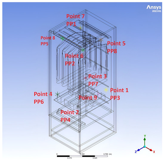
Figure 2.
Selected points of the simulation area corresponding to the experimental measurements.
For the development of the simulation model, three turbulence models were considered.
K-epsilon turbulence model: This model is applied exclusively to fully turbulent flows and is less effective for complex flows with strong pressure gradients and phenomena that occur in the boundary layer [13].
K-omega turbulence model: This model is known for its high efficiency compared with models in the k-epsilon group when simulating phenomena in the boundary layer and disturbances of the flow. However, it performs less effectively in fully turbulent flows.
Transition SST model: This model is based on coupling the transport equations of the SST k-omega model with two additional transport equations, one for the intermittency criteria and one for the onset of transition, based on the Reynolds number. A proprietary empirical correlation by ANSYS (Langtry and Menter) has been developed to account for a standard transition bypass, as well as flows in low-turbulence free-stream environments [14].
The simulation was carried out in five steps for the three turbulence models, with the aim of determining the most accurate and temporally efficient solution for the drying chamber.
- Resolution of the mesh and method of creating cells: linear without mid-side nodes, and quadratic with mid-side nodes. The number of iterations remained constant at 100.
- Gas models: ideal gas, incompressible gas, constant density.
- Iterations of the simulation: 100/500/1000
- Combined simulations: combining simulations with the minimum and maximum number of iterations with the simulation having the highest resolution and the maximum number of mesh elements.
The number of iterations of the simulation determines how many times the simulated system or model will be updated during the simulation. Each iteration represents a time step when the change in the model’s state is calculated on the basis of the boundary conditions and the defined parameters of the simulation. In practice, a higher number of iterations can result in a more detailed and precise simulation, but it also requires greater computational resources. The impact of the number of iterations also depends on the phenomenon being modelled. Some processes require smaller time steps to accurately replicate their behaviour.
4. Experimental Investigations of the Drying and Sanitising Cabinet
The experiments were conducted in a climatic chamber maintaining conditions corresponding to climate Class III:
- Air temperature: 25 °C;
- Relative humidity: 60%.
The set temperature point in the device was 40 °C, and the air humidity was set to 20%. The drying process ended when the set relative humidity was reached.
Inside the cabinet, 12 temperature sensors (T1…T12) and 9 omnidirectional air velocity measurement probes (PP1…PP8) were placed, alongside 12 humidity sensors (P1…P12). Figure 3 shows the scheme of connecting the sensors to the data loggers.

Figure 3.
Electrical wiring diagram of the test bench. 1, computer with Windows system; 2, analogue signal converter (MaxMod Ax); 3,Comet MS6D datalogger; 4, 24 V/100 W power supply, 5, Arduino Mega 2560 Rev3; a, HD103T airflow probe; b, temperature sensor; c, SHT030 humidity sensor.
Measurements were also taken with an airflow probe at the inlet of the heat pump to determine whether the airflow’s velocity was uniform throughout the length of the suction channel.
Details of the measuring instruments are shown in Table 3. The distribution of the measurement points corresponding to the points in the simulation is shown in the photograph in Figure 4.
Table 3.
Parameters of measurement devices’ setup.
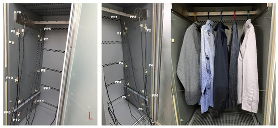
Figure 4.
Arrangement of the sensors in the drying chamber during measurements. P1–P12: temperature sensors, PP1–PP8: velocity probes.
The preparation for the measurements included the preparation of the charge by soaking five shirts in 1.2 L of water before each measurement cycle. The chamber was placed, as mentioned above, in a measurement channel with established conditions in Zone III. Measurements were carried out until the assumed removal of moisture (drying) from the load. The velocities measured during drying fluctuated, as shown in Figure 5 and Figure 6.

Figure 5.
Short-term variations in the value of air velocity measured during the measurements.
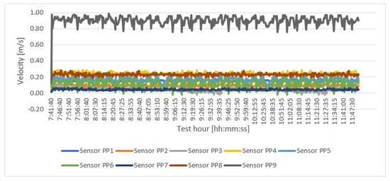
Figure 6.
Air velocity readings during long-term measurements.
The air velocities during the measurement were averaged over the measurement time, and the average values for several measurement cycles were calculated and shown in Table 4.
Table 4.
Average values of speed at specified measurement points.
5. Discussion of the Results of the Simulation Model
The following shows how the selection of the model’s parameters for the simulation was carried out. Table 5, Table 6, Table 7, Table 8 and Table 9 show the simulation’s results for different meshes, enclosing models, and numerical parameters. In each table, the highlighted column is the one with the results for which the parameters used for the simulation were considered to give the best result in terms of accuracy and computational speed. During the simulation, increasing the number of iterations resulted in simulation errors, which were attributed to the insufficiently accurate mesh of the model. Table 5 shows the impact of the number of iterations per computational step with the constraint of 100/500/1000 iterations. In this computational range, as can be seen, realistic results were obtained only for the k-omega turbulence model.
Table 5.
Results of the simulation for changes in the number of iterations of the simulation.
Table 6.
Results of the simulation for refinement of the computational grid with different turbulence models.
Table 7.
Effect of the number of iterations and the density of the mesh on the results of the simulation for different turbulence models.
Table 8.
Results of the simulation for different gas models (ideal gas and the constant-density gas).
Table 9.
Simulation results for different gas models (ideal and incompressible gas).
Table 6 shows the effect of the type and refinement of the grid on the precision of the results. By changing the grid’s resolution (number of resolutions), the grid was densified, which increased the simulation time, and the method of creating cells was linear/quadratic. During the simulation, the variables were the turbulence models, the grid models, and the number of analyses. The simulation’s results are presented in the Table 6.
The next step of the simulation involved combining the simulations with 100/1000 iterations and the simulations with the highest number of grid elements. Simulations were conducted for three turbulence models. The results are presented in Table 7.
The effect of the gas model on the simulation’s results was analysed further. Three gas models were compared: ideal gas, incompressible gas, and constant-density gas. The results are shown in Table 8 and Table 9. The type of grid and the number of iterations were selected in the previous simulations. Table 8 shows the differences in the results and the simulation time for the ideal gas and the constant-density gas.
The last simulation that was conducted was for an incompressible gas. The Table 9 below presents a comparison of the simulations for an incompressible gas and for a perfect gas.
After conducting the simulations, the average percentage of error of the measurements was calculated compared with empirical studies, as presented in Figure 7.
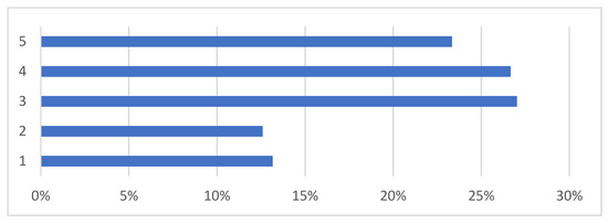
Figure 7.
Percentage differences between the simulation’s results and the experimental measurements. (1) Constant density + 1000 iterations + resolution 7 + linear; (2) constant density + 100 iterations + resolution 7 + linear; (3) ideal gas + 100 iterations + resolution 6 + quadratic; (4) ideal gas + incompressible + 100 iterations + resolution 6 + quadratic; (5) constant density + 100 iterations + resolution 6 + quadratic.
Very similar results in terms of deviation from the experimental data were obtained for 100 and 1000 iterations. However, due to considerations of computational time, shown in Figure 8, a simulation with grid refinement at a level of 7 and 100 iterations was selected. The following chart compares empirical studies with the simulation mentioned above.
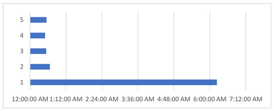
Figure 8.
Average simulation time. (1) Constant density + 1000 iterations + resolution 7 + linear; (2) constant density + 100 iterations + resolution 7 + linear; (3) ideal gas + 100 iterations + resolution 6 + quadratic; (4) ideal gas + incompressible + 100 iterations + resolution6 + quadratic; (5) constant density + 100 iterations + resolution 6 + quadratic.
The average difference between the selected simulation and the empirical studies was approximately 10%, as shown in Figure 9. For further simulations regarding the optimisation of the cabinet, the simulation with the k-omega turbulence model, a resolution level of 7, linear cell creation, and a model of constant-density gas was adopted, as it proved to be the most favourable simulation in terms of time and accuracy. Figure 10 shows a depiction of the model cabinet during the simulation using the chosen method.
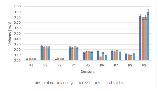
Figure 9.
Comparison of empirical studies with the selected simulation with the highest grid resolution and 100 iterations (own study).
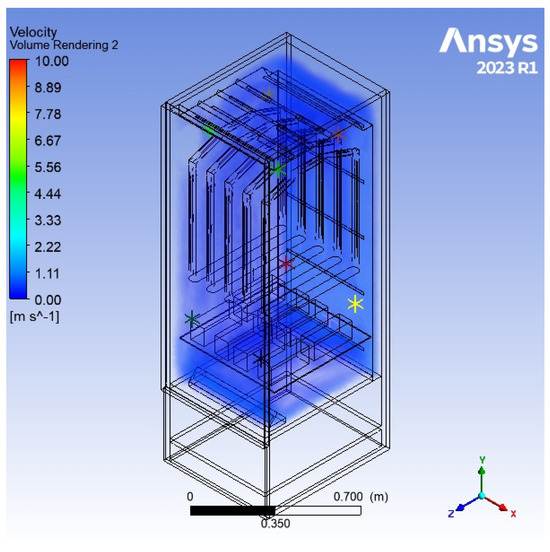
Figure 10.
Results of the 3D model of the cabinet, showing the values of velocity using the chosen method.
The experimental results confirmed the simulation’s calculations, since in both the simulation’s results and the experiment, the distribution of velocity in the chamber was highly uneven. This means that correction of the geometry would be necessary to achieve better drying results. The selected parameters of the simulation model, experimentally confirmed, were a useful tool to obtain the computationally correct geometry. The parameters of the selected simulation are presented in Table 10.
Table 10.
Parameters of the selected simulation.
6. The Shape of the Innovative Chamber and Its CFD Optimisation
After the basic chamber had been tested, an innovative design of the air’s distribution for drying was made. Additional blowing channels were added inside the clothes to allow the distribution of air inside the clothes. In the new design, clothes are dried from the outside and from the inside. The circulation of air inside the closet was redesigned, the heat pump’s air outlet was moved to the front of the unit, and the heat pump’s air intake was moved to the back of the unit. The unit operates in a closed air cycle. Figure 11 shows the cabinet after the changes to the design. The shape of the blowing channels mades it possible to dry shirts and pants.
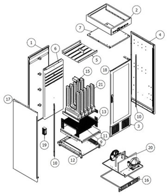
Figure 11.
Innovative design of the drying cabinet. (1) Back of the chamber; (2) control panel; (3) front panel; (4) right side of the chamber; (5) top of the perforated sheet for ozone supply; (6) rear perforated sheet for air suction; (7) ceiling of the chamber; (9) sheet for blowing air; (10) LED lighting; (11) bottom of the chamber; (12) base of the cabinet; (13) shoe shelf; (15) ozone generator; (16) drip tray; (17) left side of the chamber; (18) glass door; (19) electromagnetic lock; (20) air duct partition, (21) assembly of the clothes channel.
Optimisation of the distribution of the perforations in the channels for blowing the clothes was carried out using the determined and verified model shown above. Ten different versions of the distribution of perforations for the garment-dodger’s channels were designed and studied. In the figures below, the distribution of perforation for the most uniform and least uniform distributions of air velocity throughout the studied area of the drying chamber is shown. In the first version, the inward blowing channels had perforations with a uniform distribution of holes. In the second version, the distance between the perforations increased by 7.5 mm from the outermost perforation.
The innovative version of the dryer has additional blowing channels (Figure 12) powered by small fans that also allowed circulating drying air to be introduced into the dried clothes as well. These channels were designed to allow both hanging shirts or jackets and upside-down pants. They were developed in order to homogenise the speed of the drying air, and they also have an important sanitising function, allowing the introduction of ozone into the clothes. Table 11 shows the boundary conditions of the blowing channels.
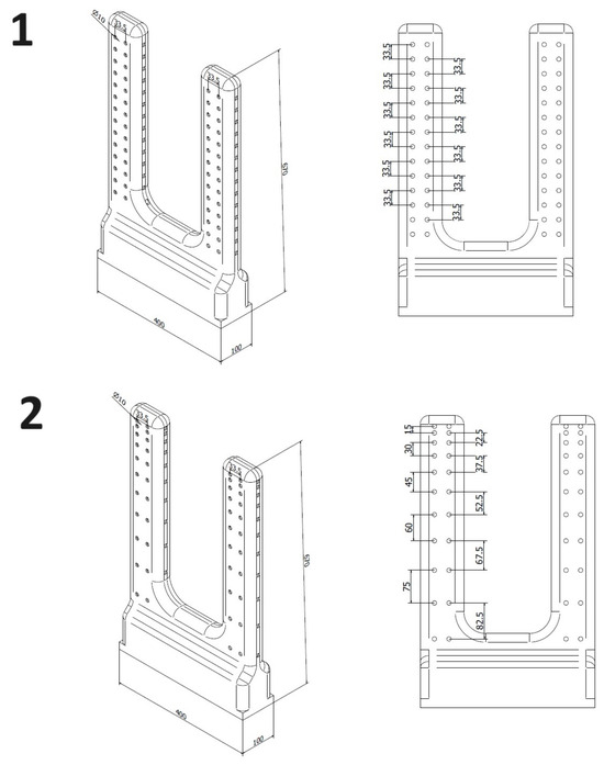
Figure 12.
Two versions of an example of the arrangement of blowing channels. (1) uniform distribution, (2) exponential distribution.
Table 11.
The simulation’s boundary conditions.
In the simulation of a single blowing channel, the characteristic measurement points (nine points) were plotted to compare the calculated and measured distributions of air velocity. The locations of the measurement points for a single channel (shown as a horizontal layout) are shown in Figure 13.
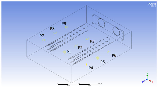
Figure 13.
Characteristic points for CFD simulations of the blowing channels. P1–P9 points corresponding to measuring points in which values of simulated air velocity are precisely tracked.
Figure 14 and Figure 15 show the results of the simulation for Versions 1 and 2 of the blowholes’ distribution in FLUENT, which represent the distribution of air velocities from the clothes-blowing channels.
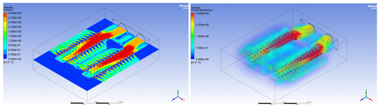
Figure 14.
Results of the simulation of the version of the clothes-blowing channel with the most uniform distribution of air velocity (Version 1).
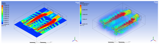
Figure 15.
Results of the simulation of the version of the clothes-blowing channel with the least uniform distribution of air velocity (Version 2).
Table 12 shows the results of the calculated average velocities at the characteristic points during the simulation.
Table 12.
Results of the calculations of speed at characteristic points.
The criterion for selecting the optimal location of the perforations was assumed to be the most uniform airflow at the characteristic points. As a result of comparing 10 different configurations of the perforation points, Version 1 was selected for the final design, as it gave the most uniform distribution of velocity. This distribution was applied to the final design of the drying and sanitising chamber. This design was also the subject of simulation using the parameters of the developed model. As before, eight characteristic points were chosen for experimental verification of the results (Figure 16), and air velocity results presented in Figure 17).
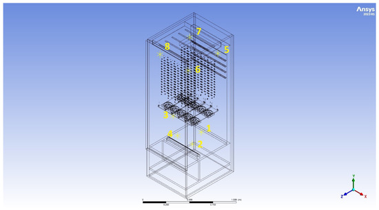
Figure 16.
Characteristic points (1–8) of air velocity in the simulation area corresponding to the experimental measurements.
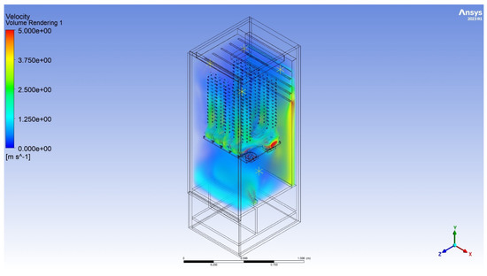
Figure 17.
Results of the simulation of air velocity for a new optimised geometry of the drying–sanitising chamber.
In Table 13 and Figure 18, a comparison between the simulation and the experimental results for the magnitude of velocity is presented. The average difference between the magnitudes was about 6%. Measurements Points 1–4 were located closest to the air exhaust of the heat pump, while Points 5–8 were located at the top of the closet just behind the clothes-blowing channels.
Table 13.
Comparison of the simulated and measured (averaged) magnitudes of velocity at characteristic points.
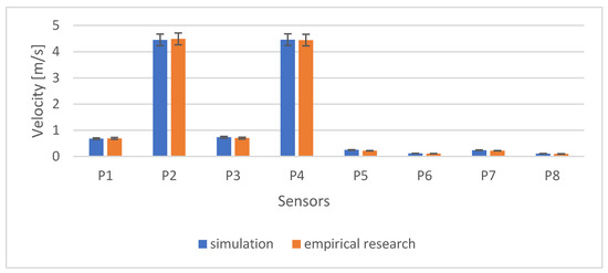
Figure 18.
Comparison of simulated and measured (averaged) magnitudes of velocity at characteristic points.
Figure 19 shows the mapping of the measurement points of empirical research in the model during the CFD simulation.
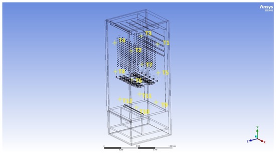
Figure 19.
Characteristic points of air temperature (T1–T12) in the simulation area corresponding to the experimental measurements.
To further verify the simulation’s results, the results of measuring the temperature were compared with the simulation’s results at the measurement points shown in Figure 20. A comparison of the results is shown in Table 14 and Figure 21. The results of the transient distribution of temperature in the simulation are shown in Figure 20.
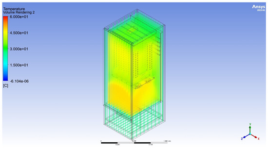
Figure 20.
Results of the simulation of the air temperature for the new optimised geometry of the drying–sanitising chamber.
Table 14.
Comparison of the simulated and measured (averaged) temperatures at the characteristic points.
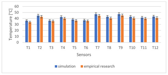
Figure 21.
Comparison of the simulated and measured (averaged) temperatures at the characteristic points.
In Table 14 and Figure 21, a comparison between the simulation and the experimental results for temperature is presented. The average difference between the temperatures was about 5%.
The base version of the cabinet design shown at the beginning of the article was inefficient. After approximately 2 h of testing, about 0.5 kg of water was condensed from the clothes, and the measured relative humidity dropped from the initial 65% to 45%. Optimisation of the drying cabinet, including the innovative design of the geometry of the drying chamber and customised optimisation of the heat pump’s supply, allowed the shortening of the drying process to 50 min, achieving condensation of 0.8 kg of water and a relative humidity at the measured point of approximately 28%. The course of the measurements of the average relative humidity during the drying process for both designs is shown in Figure 22.

Figure 22.
Average relative humidity during drying: A, chamber with the optimised innovative design geometry; B, standard (initial) design.
7. Conclusions
The article presents an innovative design of the geometry of a drying–sanitising chamber. Optimisation of the chamber’s shape required the development of a simulation model and its experimental verification. On the basis of many simulations for different versions of both the air-drying models and the numerical options, it was concluded that the following model would be used for further calculations: a structural mesh, a mesh with a resolution at Level 7, a linear method of creating the mesh cells method, gas with a constant density, and 100 iterations.
The model chosen in this way gave simulation results close to the experimental measurements, and the computation time on a PC-class server with Intel Xeon 6242R prossesor (Intel Corporation, Santa Clara, CA, USA) was acceptable.
The developed model optimised the distribution of perforations in the blowing channels that recirculated the drying air inside the drying chamber. The criterion for optimisation was to achieve the most uniform distribution of air velocity possible. The requirement for the uniformity of the distribution of velocity was due to both the drying process and the need to supply ozone to each part of the drying clothes. At the same time, the heat pump supply was optimised, which allowed a definite overall improvement in the operation of the drying and sanitising chamber, reducing the drying time and electricity consumed by more than twofold.
The methodology presented here for modelling and optimisation of the shape can be applied to different sizes of drying and sanitising devices where an important element is to achieve a uniform distribution of air.
Author Contributions
Conceptualisation, D.C. and P.C.; methodology, formal analysis, investigation, writing—review and editing, and supervision, P.C.; validation, resources, data curation, writing—original draft preparation and visualisation, D.C. All authors have read and agreed to the published version of the manuscript.
Funding
This work was supported by the Ministry of Science and Higher Education of the Republic of Poland (IVth edition DWD/4/25/2020) and this research was carried out with the support of the ANSYS National Licence coordinated by Interdisciplinary Centre for Mathematical and Computational Modelling University of Warsaw (ICM UW).
Institutional Review Board Statement
Not applicable.
Informed Consent Statement
Not applicable.
Data Availability Statement
The data presented in this study are available on request from the corresponding authors.
Acknowledgments
Special thanks to JUKA Company for the technical support and sharing of their climate chamber for the experimental tests.
Conflicts of Interest
The authors declare no conflicts of interest.
References
- Janusz, S.; Szudarek, M.; Rudniak, L.; Borcuch, M. Analiza parametrów cieplno-przepływowych lamelowego wymiennika ciepła z wykorzystaniem pełnowymiarowego modelu CFD i jego weryfikacji eksperymentalnej. Instal 2022, 6, 29–34. [Google Scholar] [CrossRef]
- Stribling, D. Investigation into the Design and Optimisation of Multideck Refrigerated Display Cases. Ph.D. Thesis, Department of Mechanical Engineering, Brunel University, Uxbridge, UK, 1997. Available online: https://api.semanticscholar.org/CorpusID:107707490 (accessed on 13 November 2023).
- Mołczan, T.; Cyklis, P. Impact of the Evaporation Temperature on the Air-Drying Rate for a Finned Heat Exchanger. Energies 2023, 16, 2132. [Google Scholar] [CrossRef]
- Ryu, J.-B.; Jung, C.-Y.; Yi, S.-C. Three-dimensional simulation of the humid-air dryer using computational fluid dynamics. J. Ind. Eng. Chem. 2013, 19, 1092–1098. [Google Scholar] [CrossRef]
- Al-Kayiem, H.H.; Gitan, A.A. Flow uniformity assessment in a multi-chamber cabinet of a hybrid solar dryer. Sol. Energy 2021, 224, 823–832. [Google Scholar] [CrossRef]
- Dasore, A.; Konijeti, R. Numerical Simulation of air Temperature and airflow Distribution in a Cabinet tray Dryer. Int. J. Innov. Technol. Explor. Eng. 2019, 8, 1836–1840. [Google Scholar] [CrossRef]
- Pintanaa, P.; Thanompongchart, P.; Phimphilai, K.; Tippayawong, N. Improvement of Airflow Distribution in a Glutinous Rice Cracker Drying Cabinet. Energy Procedia 2017, 138, 325–330. [Google Scholar] [CrossRef]
- Sun, J.; Tsamos, K.M.; Tassou, S.A. CFD comparisons of open-type refrigerated display cabinets with/without air guiding strips. Energy Procedia 2017, 123, 54–61. [Google Scholar] [CrossRef]
- Titariya, V.K.; Tiwari, A.C. Parametric Investigation of the Air Curtain for Open Refrigerated Display Cabinets. Int. J. Soft Comput. Eng. 2012, 2, 121–126. [Google Scholar]
- Ambarita, H.; Nasution, A.H.; Siahaan, N.M.; Kawai, H. Performance of a clothes drying cabinet by utilizing waste heat from a split-type residential air conditioner. Case Stud. Therm. Eng. 2016, 8, 105–114. [Google Scholar] [CrossRef]
- Zhao, H.-B.; Wu, K.; Zhang, J.-F. Simulation Study on Active Air Flow Distribution Characteristics of Closed Heat Pump Drying System with Waste Heat Recovery. Energies 2021, 14, 6358. [Google Scholar] [CrossRef]
- Wang, D.; Tan, L.; Yuan, Y.; Lu, Y. CFD simulation and optimization on airflow uniformity of material drying room used in steam blanching and hot-air vacuum drying equipment. J. Mech. Sci. Technol. 2023, 37, 5463–5474. [Google Scholar] [CrossRef]
- K-Epsilon Turbulence Models. Available online: https://www.simscale.com/docs/simulation-setup/global-settings/k-epsilon/ (accessed on 13 November 2023).
- Reid, K.E. Numerical Simulation Using Transition SST Model to Analyze Effects of Expanding. Manifold Angle and Jet Spacing for Submerged Liquid Jet Impingement. Ph.D. Thesis, Auburn University, Auburn, AL, USA, 2018. Available online: http://hdl.handle.net/10415/6330 (accessed on 13 November 2023).
Disclaimer/Publisher’s Note: The statements, opinions and data contained in all publications are solely those of the individual author(s) and contributor(s) and not of MDPI and/or the editor(s). MDPI and/or the editor(s) disclaim responsibility for any injury to people or property resulting from any ideas, methods, instructions or products referred to in the content. |
© 2024 by the authors. Licensee MDPI, Basel, Switzerland. This article is an open access article distributed under the terms and conditions of the Creative Commons Attribution (CC BY) license (https://creativecommons.org/licenses/by/4.0/).