Prediction of Mean Heat Transfer Characteristics of Multiple Impinging Jets with Steady RANS Simulation Using a Coarse Mesh

Abstract

The capability of the standard SST k-ω turbulence model for the prediction of jet impingement cooling characteristics using a coarse mesh is investigated. The discussion is based on a sensitivity study with five computational grids, differing from each other in topology and resolution. The analysis considers a hexagonal configuration of turbulent jets at the inlet Reynolds number equal to 20,000, with the distance between the nozzle and target plates equal to four nozzle diameters. The results of steady RANS simulations are validated against the time-averaged LES results and data from experiments. The mean heat transfer characteristics of turbulent impinging jets have been successfully reproduced with all tested grids, which indicates that for a rather accurate mean heat transfer prediction, it is not necessary to resolve all the small-scale flow features of impinging jets above the target plate.

1. Introduction

Turbulent impinging jets exhibit intricate flow dynamics and remarkable heat transfer characteristics, rendering them highly favored for cooling applications [1], and at the same time, present a challenging case to test statistical turbulence models [2,3]. At sufficiently high Reynolds numbers, the flow experiences shear-driven instabilities, caused by steep velocity gradients. Initially, small disturbances at the edges of the jet undergo significant growth, leading to the formation of the so-called shear layer. In configurations with multiple jets, the flow near the impingement surface is additionally disrupted due to collisions between neighboring wall jets. These processes collectively contribute to highly intense and chaotic flow dynamics near the impingement wall. The growth of the thermal boundary layer is constantly perturbed by oscillating jets and intense periodic occurrences of large-scale vortical structures [4]. These phenomena have been identified as the most important mechanisms governing the localized enhancements in heat transfer [4]. The mean (i.e., time-averaged) heat transfer characteristics of multiple impinging jets demonstrate maximum values within the impingement zones of individual jets, where the aforementioned mechanisms are statistically the most frequent.

Our interest in jet impingement cooling arises from the optimization studies of the Helium-Multiple Jet (HEMJ) DEMO divertor design [5], where the plasma-facing target plates of diverter cassettes are proposed to be assembled from numerous cooling fingers, each of them facilitating the multiple helium jets for the cooling. The term “DEMO” in the context of nuclear fusion refers to a demonstration power plant that is intended to be the next step beyond the experimental or prototype fusion reactors (like ITER and JET), which are being designed to demonstrate the feasibility of continuous and sustainable nuclear fusion as a viable energy source [6].

To complement the rather lacking literature and understanding of physics associated with multiple impinging jets, Large Eddy Simulation (LES) studies of the experimental case with 13 turbulent impinging jets in hexagonal arrangements have been initiated [4]. A few years ago, generating high-quality (hexahedral) structured mesh in complex finger geometry was a challenging task since meshing was not a fully automated process, thus requiring a vast amount of skills and time. Nowadays, it is often stated that a completely automated polyhedral meshing may represent a good and time-saving alternative in practice, as it requires very few user interventions to build an adequate mesh. As such, the performance of a representative polyhedral mesh is also tested in this study.

In our previous studies [4], we have successfully utilized the Large Eddy Simulation (LES) to accurately simulate the instantaneous flow and heat transfer characteristics of multiple turbulent impinging jets. These investigations provided valuable insights into the significance of large-scale flow structures in the dynamics of near-wall flow. Key flow phenomena associated with single and multiple turbulent impinging jets have been rather accurately predicted [4], such as the enhanced production of wall-normal and shear stresses across the stagnation region and the shear layer of individual jets. To sufficiently resolve the occurring flow phenomena by the LES, high fidelity (spatial and temporal) discretization is needed, which makes the LES of turbulent impinging jets computationally very demanding.

Flow statistics and turbulence budgets of impinging jets can be rather accurately modeled by the unsteady Reynolds averaged Navier-Stokes (URANS) approach with the conventional eddy-viscosity turbulence models [7,8,9,10,11]. However, the simulations conducted with the Shear Stress Transport (SST) model [12] and the SST-based Scale-Adaptive Simulation model (SST-SAS) model [13] exhibit a tendency to completely suppress the flow unsteadiness near the target plate [14,15]. In comparison to the LES, one order of magnitude higher eddy viscosity values have been obtained with both the SST and the SST-SAS turbulence models. Since the grid resolution across the individual jets was kept similar to the coarsest LES grids [4,16], a small time step of the simulation, comparable to LES, was needed to obtain the solver convergence. Yang [17] simulated the twin impinging jets in a cross-flow with the RANS and URANS approaches using the RMS turbulence model and observed an increase in computational costs by a factor of five for the URANS simulations. While both simulation approaches relatively well predicted the mean flow field, superior predictions of wall-normal stresses have been observed with the URANS simulations. Barata et al. [18] in their study of a confined slot turbulent jet observed that steady RANS simulations yield fairly good results only for low nozzle-to-plate distances, while for configurations with confinement heights, greater than five nozzle diameters the LES is needed to capture the unsteady jet flapping that governs the statistics of ensemble-averaged quantities.

A good alternative to LES methods in terms of reduced computational costs are also the so-called hybrid RANS/LES models. Martínez-Filgueira et al. [19] studied a 3 × 3 square set-up nozzle array impinging jet system at Reynolds number around 8500 by the means of five different turbulence modeling techniques, including the hybrid RANS/LES approach-Detached Eddy Simulation (DES). They reported the superior behavior of the LES technique and the need for a high-resolution mesh over the entire domain in order to capture the essential flow features. Kubacki and Dick [20] reported that a fine mesh is required for the hybrid RANS/LES models to improve the RANS prediction by resolving the dynamics of large-scale vortical structures in the shear layer and in the near-wall region. Wu and Piomelli [21] reported that both the Wall modeled LES (WMLES) and the Delayed Detached Eddy Simulation (DDES) are able to predict vortex decay, which is in good agreement with the well-resolved LES data.

These observations call into question the feasibility of unsteady RANS and hybrid RANS/LES simulations of impinging jets in terms of the required additional computational effort compared to a steady-state approach, which is an important constraint/aspect of industrial CFD applications.

With respect to the selection of the RANS turbulence model, the two-equation SST model by Menter [22] and Durbin’s four-equation $v^2-f$ model [23,24] have been acknowledged as the most successful in the reproduction of the flow and heat transfer characteristics of turbulent impinging jets [21,25,26,27]. However, the $v^2-f$ model may exhibit pseudo-transitional behavior that is not calibrated against data and, as such, is no longer available in the ANSYS CFD codes, including the ANSYS Fluent R21.2 [28,29].

With the above in mind, this work investigates the predictive capability of the steady RANS approach with the SST k-ω model for modeling the mean heat transfer characteristics of highly turbulent multiple impinging jets. Aiming at industrial CFD applications where automated meshing is desirable, the goal of this study is to demonstrate how the mesh resolution and topology affect the predicted mean flow and heat transfer characteristics. Five different computational grids of two different topologies (structured hexahedral and unstructured polyhedral) are tested, with varying cell resolution across the diameter of the jets and near the impingement wall. Results are compared with the existing LES [4,16] and experimental data [30,31,32]. The area-weighted average temperature of the target plate is reported together with the stagnation point wall temperature, which may be used for a quantitative assessment of the cooling efficiency of a method in practice. An analysis is conducted for a configuration with 13 turbulent jets in a hexagonal arrangement at an inlet Reynolds number equal to 20,000 and a confinement height equal to four nozzle diameters (i.e., for the experimental test case by Geers [30,31,32]). Contrary to our previous URANS studies of multiple impinging jets that have been conducted with the OpenFOAM code [15], this study is performed with the commercial code ANSYS Fluent R21.2 [33].

The structure of the paper is the following: the test case is presented in Section 2, while information about the numerics and the simulation setup is given in Section 3. The results are presented in Section 4. The conclusions are drawn in Section 5.

2. Test Case (Benchmark Data)

The considered case was originally studied experimentally by Geers [30,31,32], who conducted the measurements of the flow field with Particle Image Velocimetry (PIV) and Laser Doppler Anemometry (LDA). The temperature distribution at the impingement sheet was determined with Liquid Crystal Thermography (LCT). The airflow with a controlled mass flow rate was supplied through a squared cross-section wind tunnel to a nozzle plate with a thickness of $2\mathrm{mm}$. The reported Reynolds number at the nozzle plate is equal to 20,000 [31]. The flow field measurements were taken only within the confinement between the nozzle plate and the impingement sheet (see Figure 1), i.e., the experimental velocity and turbulence conditions at the nozzle lip are not reported. The dimensions of the squared nozzle plate are reported to be $0.3 \mathrm{m}\times 0.3\mathrm{m}$, while the height of the confinement (i.e., nozzle-to-plate distance) is reported to be $0.052 \mathrm{m}$.

The used LES benchmark data [16] have been obtained with the second-order accurate in-house code PSI-BOIL (Parallel SImulator of BOILing phenomena) [34]. The LES study with the explicit Wall-Adaptive Local Eddy (WALE) viscosity sub-grid-scale (sgs) model [35] considers only the part of the experimental apparatus after the nozzle plate (see Figure 1). Reported uncertainties of statistically averaged LES results, associated with the grid refinement and due to sampling statistics and variation of the sgs constant, are in the order of ten percent for the mean flow characteristics, while the uncertainty of the mean wall temperature is estimated to be less than two percent [16]. Additional information about the LES setup is available in [4,16].

3. Simulation Details

The incompressible fluid flow of impinging jets has been simulated with the commercial CFD code ANSYS Fluent R21.2 [36], using the steady-state RANS approach. The effects of turbulence are modeled using the two-equation eddy viscosity Shear-Stress Transport (SST) k-ω model [12], which automatically activates y⁺-insensitive wall-treatment [33]. The working fluid is air, which is modeled with constant thermophysical properties [16]. The fluid density $\rho$ is set to $1.2047 \mathrm{kg}/{\mathrm{m}}^3$, the dynamic viscosity is set to $1.8204\cdot {10}^{-5} \mathrm{kg}/\left(\mathrm{m}\mathrm{s}\right)$, the thermal conductivity of air is set to $0.0256 \mathrm{W}/\left(\mathrm{m}\mathrm{K}\right)$ and the specific heat is set to $1006.1 \mathrm{J}/\left(\mathrm{kg}\mathrm{K}\right)$.

3.1. Governing Equations

For steady-state incompressible fluid flow, the Reynolds-averaged Navier-Stokes (RANS) equations in Cartesian tensor form read as [33]:

$$\frac{\partial \overline{u_i}}{\partial x_i}=0$$

(1)

$$\frac{\partial }{\partial x_i}\left(\rho \overline{u_i}\overline{u_j}\right)=-\frac{\partial \overline{p}}{\partial x_i}+\frac{\partial }{\partial x_j}\left[\mu \left(\frac{\partial \overline{u_i}}{\partial x_j}+\frac{\partial \overline{u_j}}{\partial x_i}\right)\right]+\frac{\partial }{\partial x_j}\left(-\rho \overline{u_i^{\prime }{u}_j\prime }\right)$$

(2)

where $\overline{u_i}$ is the mean (Reynolds averaged) velocity component in $i$-th direction, $x_i$ is the $i$-th spatial coordinate, $\overline{p}$ is the mean pressure, and $\mu$ is the molecular viscosity. The last term on the right-hand side of Equation (2) represents the Reynolds stresses, which are modeled with the turbulence model. In the SST k-ω model, the Boussinesq hypothesis is used. Thus, the Reynolds stresses are computed from mean velocity gradients [33]:

$$-\rho \overline{u_i^{\prime }{u}_j\prime }={\mu }_t\left(\frac{\partial \overline{u_i}}{\partial x_j}+\frac{\partial \overline{u_j}}{\partial x_i}\right)$$

(3)

where the eddy viscosity ${\mu }_t$ is computed from the turbulence kinetic energy $k$ and the specific dissipation rate $\omega$.

The turbulent heat transport in incompressible fluid flow is described with the following energy equation [33]:

$$\frac{\partial }{\partial x_i}\left[\overline{u_i}\overline{T}\right]=\frac{\partial }{\partial x_j}\left[\left(\alpha +{\alpha }_t\right)\frac{\partial \overline{T}}{\partial x_j}\right]$$

(4)

where $\overline{T}$ is the mean temperature, $\alpha$ is the thermal diffusivity, and ${\alpha }_t$ is the turbulent thermal diffusivity; the latter is computed from eddy viscosity ${\mu }_t$ and turbulent Prandtl number $P{r}_t$. In this study, the turbulent Prandtl number is set to 0.9.

Turbulence properties $k$ and $\omega$ are calculated using the Shear-Stress Transport (SST) $k-$ω turbulence model [12]. The eddy viscosity is computed as [33]:

$${\mu }_t=\frac{\rho k}{\omega }\frac{1}{\max \left[\frac{1}{{\alpha }^{*}},\frac{S{F}_2}{{\alpha }_1\omega }\right]}$$

(5)

where $S$ is the strain rate magnitude and ${\alpha }^{*}$ is the damping coefficient causing a low-Reynolds number correction [33]. $F_2$ is given by

$$F_2=\tanh ({\left(\max \left[2\frac{\rho \sqrt{k}}{0.09\omega y},\frac{500\mu }{\rho y^2\omega }\right]\right)}^2)$$

(6)

where $y$ is the distance from the field point to the nearest wall [37]. A detailed description of the SST $k-$ω turbulence model is available in the code documentation [33].

3.2. Numerics

The Pressure-Based Coupled Algorithm with the pseudo-transient under-relaxation method is used to solve the steady-state form of RANS equations [36]. Spatial discretization of gradients is obtained with the default gradient method “Least Squares Cell Based”, and the pressure is discretized with the “Second Order” scheme. The “Second Order Upwind” scheme has been selected for the discretization of governing equations for momentum, energy, turbulence kinetic energy, and specific dissipation rate. Due to the very high aspect ratio of cells at the impingement wall, a Warped-Face Gradient Correction (WFGC) method is enabled [38].

In order to avoid the excessive generation of the turbulence energy ($G_k$) in the stagnation regions, the production limiter is used (default feature in Fluent for SST k-ω model) [33]:

$$G_K=\min \left[G_k,C_{\lim }\rho \epsilon \right]$$

(7)

where $\rho$ is the fluid density and $\epsilon$ is the turbulent dissipation rate. The coefficient $C_{\lim }$ is set to its default value of ten [33]. According to the ANSYS documentation [33], the usage of this limiter seems like a reasonable choice for simulations of impinging jets as, by definition, the limiter prevents excessive turbulence production in the stagnation region, while the turbulence model performance in the shear flow remains intact. The need for the turbulence production limiter within the SST turbulence model has been demonstrated in our previous study [39], where it has been shown that the Kato-Launder production limiter [40] eliminates excessive turbulence production in the stagnation region of a single jet and improves the heat transfer prediction.

3.3. Geometry

The three-dimensional simulation domain, shown in Figure 2, has dimensions similar to the LES benchmark [4,16]. The air inflow occurs through the 13 circular inlets at the nozzle plate (inlet). The outflow is established through four vertical boundary planes (outlets). The diameter of individual nozzles ($D$) is equal to 0.013 m, the distance between nozzles is equal to $2D$, and the nozzle-to-plate distance is equal to four nozzle diameters. Additional information about the simulation case (including LES setup) can be found in [4,16].

3.4. Boundary Conditions

At the inlet, a velocity inlet boundary condition with a velocity magnitude equal to $23.88 \mathrm{m}/\mathrm{s}$ and turbulence intensity of 10% is applied [15]. The temperature of the inflowing air is equal to 20 °C. A no-slip wall boundary condition is used for the nozzle plate and the target surface. The applied heat flux at the target wall is set to 905 $\mathrm{W}/{\mathrm{m}}^2$ [16]. The outlet is modeled with the pressure outlet condition. The backflow turbulent intensity is set to 1%, and the backflow turbulent length scale is set to $0.013 \mathrm{m}$.

3.5. Computational Grid

Five different computational grids were tested in this study, with the total number of cells ranging from $1,550,217$ to $4,219,879$. The grids differ from each other in resolution, topology (fully structured hexahedral vs. unstructured polyhedral cells), and near-wall spacing (i.e., the height of the first cell is varied to obtain various $y^{+}$ at impingement surfaces). For accurate heat transfer predictions, the near-wall meshes of $y^{+}~1$ are recommended [36]. Thus, four generated grids have corresponding maximums $y^{+}<1$, while Grid G1 has the maximum $y^{+}$ equal to 4.2.

Fully structured hexahedral grids (G1 to G4) were built using the ANSYS ICEM CFD meshing tool [41]. The so-called “O-grid” blocking was generated at corresponding locations of individual jets (see Figure 3 (left)) to achieve relatively uniform grid spacing in both wall-parallel ($x-$ and $z-$) directions of the central region of the domain. A desired grid resolution near the impingement plate is achieved with additional grid refinement in the vertical direction towards both plates (see Figure 4 (left)). The fifth generated grid (G5), shown in Figure 3 (right) and Figure 4 (right), is unstructured and meshed with fully polyhedral cells with hexcore, generated using the ANSYS Fluent Meshing tool [36]. Additional information about tested computational grids is given in

Table 1. Overview of mesh parameters.

	Topology	No. of Elements	No. of Elements Across Jet	No. of Elements between Jets	No. of Elements (Vertical)	First Node Distance from Target Wall [m]	${\mathit{y}}_{\mathbf{m}\mathbf{a}\mathbf{x}}^{+}$ (Dimension-Less Wall Distance)
G1	Hexa	$1,550,217$	$23$	$17$	$80$	$2.5\times {10}^{-5}$	$4.2$
G2	Hexa	$1,550,217$	23	17	80	$5.0\times {10}^{-6}$	0.8
G3	Hexa	$3,238,684$	$30$	$30$	$80$	$5.0\times {10}^{-6}$	$0.8$
G4	Hexa	$3,238,684$	$30$	$30$	$80$	$2.5\times {10}^{-6}$	$0.4$
G5	Poly-Hexcore	$4,219,879$	15	16/4	40	$5.0\times {10}^{-6}$	0.8
LES	Hexa *	$75,497,472$	32	64	128	$1.0\times {10}^{-5}$	~1

* Structured hexa grid with uniform cells across the entire domain.

. For comparison, the grid parameters of the LES benchmark case are reported as well.

4. Results and Discussion

RANS results are validated against time-averaged data from a well-resolved LES benchmark case [4,16] and a laboratory experiment [30,31,32]. A comparison is given for several horizontal profile lines, extracted from characteristic planes P-1 and P-2. To account for the azimuthal (rotational) symmetry of 60°, each profile line is averaged over the six symmetry planes as well. Data averaging has been used in the experimental and LES analyses, as well as in the present study. The data from RANS simulations are available in supplementary material.

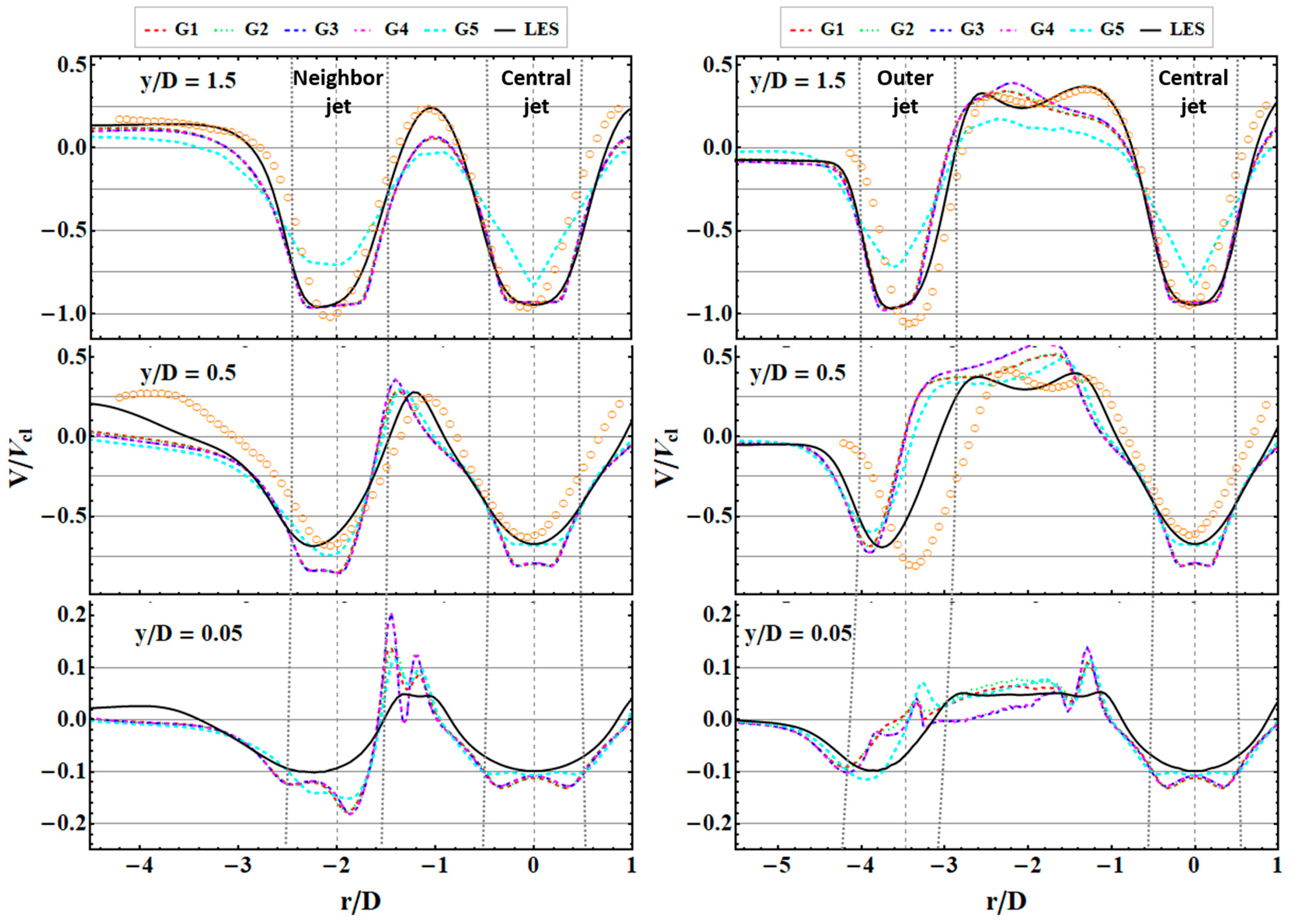
Profiles of mean axial velocity $V/V_{cl}$ in both characteristic planes P-1 and P-2 are presented in Figure 5. It is evident that all structured hexahedral grids (G1–G4) exhibit similar jet formations. The agreement with LES is notably good, particularly at locations that are distant from the target plate (e.g., $y/D=1.5$). Closer to the target wall ($y/D<0.5$), the RANS simulations predict a slightly slower decay of mean axial velocity, with the magnitude of axial velocity higher compared to that of LES.

On the other hand, the polyhedral grid (G5) insufficiently resolves the formation of jets at $y/D=1.5$. This behavior is somewhat expected, as the resolution of the polyhedral grid (G5) in the middle of the confinement is rather coarse compared to other hexahedral grids (G1–G4). In the vicinity of the target wall, for $y/D<0.5$, the magnitude of the predicted mean axial velocity at the axis of the central jet for grid G5 closely matches the LES prediction. At the same time, the predicted flow characteristics are, at locations corresponding to neighbor and outer jets, more similar to other RANS results obtained with hexahedral grids than to the results obtained with the LES.

It is also observed that all RANS simulations relatively well predict the establishment of the fountain flow between jets. Velocity magnitude is quite accurately predicted at locations that are far from the target wall (for $y/D>0.5$). Closer to the wall, at $y/D=0.05$, discrepancies between RANS and LES results are larger. This may be partly attributed to the fact that the presented LES data are computed with the statistical (time) averaging of instantaneous results of unsteady simulations, in contrast to the steady-state flow fields obtained from RANS simulations. The instantaneous flow characteristics of individual jets in LES (and in experiments) are very chaotic and unstable [4,32]. At certain instances of time, the jets become highly distorted, with impingement locations significantly dislocated from the geometrical axes of the individual jets [4]. The formation of the fountain flow has been observed from the instantaneous flow fields experimentally [32], as well as from the LES results [4]. It is acknowledged as an important mechanism that contributes to the disturbances of the jets. On the other hand, the RANS prediction represents an ensemble-averaged (statistical) realization of the flow, which never occurs in reality.

A comparison of numerical (RANS and LES) results with experimental data shows that the formation of the jets is relatively well predicted numerically near the half-height of the confinement (i.e., at $y/D=1.5$). In the characteristic plane P-1, the predicted shape of both (central and neighbor) jets closely matches the experimental observations, while in the characteristic plane P-2, a somewhat larger dislocation of the outer jet radially outward can be observed. This may be attributed to the vena contracta phenomenon, which has been observed experimentally [30], and which is not considered in the numerical simulations as the flow through the wind tunnel and nozzle is not simulated [16].

Closer to the target wall ($y/D<0.5$), a relatively good agreement between simulation results and experimental data is demonstrated for the central jet. It can be observed that the central jet is not axisymmetric in the experimental case, i.e., the reported magnitude for mean axial velocity is slightly different at both sides of the jet with respect to its geometrical axis, whereas all simulations exhibit axial symmetry for the central jet. The numerically predicted magnitude of axial velocity is in good agreement with the experimental data. Again, a notable difference in the shapes of the jets between the simulations and experiments is observed for both the neighbor and the outer jets. In the vicinity of the target wall, at $y/D=0.05$, the experimental data are not available due to the limitations of measurement techniques.

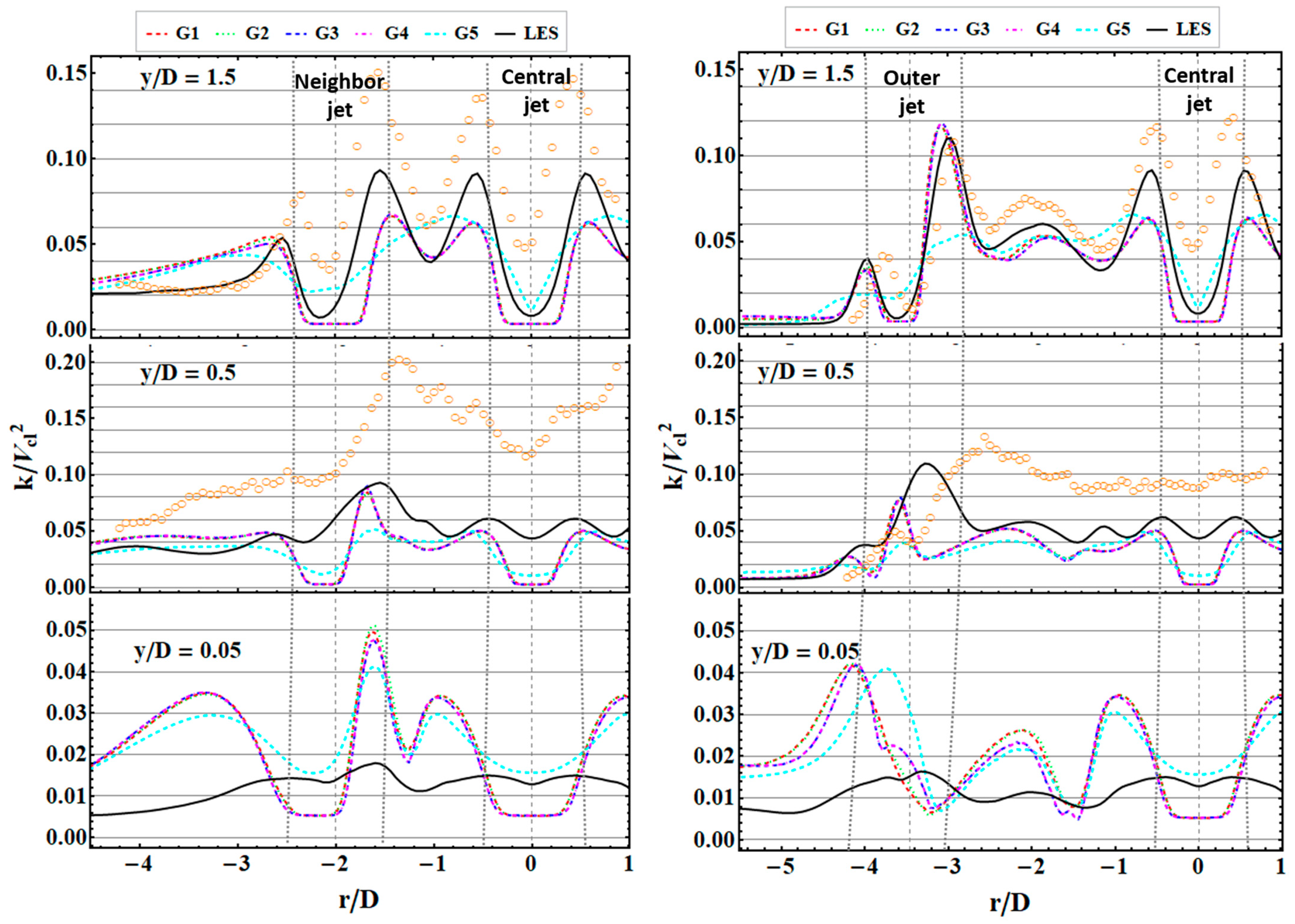
Figure 6 shows horizontal profiles of mean turbulence kinetic energy $k/V_{cl}^2$ in characteristic planes P-1 and P-2. In general, increased levels of turbulence kinetic energy occur mainly in the circumferential shear layer around the jet-core region, where the jet flow interacts with the surrounding fluid. In RANS simulations, the turbulence kinetic energy $k$ is computed with the turbulence model, while in the experimental and LES cases, k is computed from velocity fluctuations.

From Figure 6, it can be seen that all hexahedral grids predict a somewhat wider shear layer of individual jets as compared to that of the LES. At $y/D=1.5$, the occurring turbulence levels in the jet-core region of the central jet are quite low, indicating that the flow in this region is comparatively laminar. Here, the turbulence production is weak due to the low shear in the flow. In comparison to LES results, turbulence levels remain underestimated and are also closer to the target wall. On the other hand, the coarse polyhedral grid (G5) somewhat better predicts the turbulence levels in individual jets near the target wall. However, no significant differences between RANS simulations can be observed in the prediction of turbulence levels in the so-called fountain flow regions, where the values obtained by RANS simulations are comparable to those of the LES.

Compared to the experimental data, the turbulence kinetic energy is generally underpredicted by the numerical simulations. This can be mainly attributed to the lack of description of the experimental flow conditions at the nozzle lip (i.e., at the domain inlet). At $y/D=1.5$, the shear layer of experimental jets is already substantially developed. The distinguished, non-zero turbulence levels can also be observed in the jet-core region of the central jet. On the other hand, steady RANS simulations predict significantly lower levels of turbulence kinetic energy in the shear layer of individual jets and completely fail with the prediction of the mean turbulence characteristics in the jet-core region.

Closer to the target wall, at $y/D=0.5,$ the profiles of mean turbulence kinetic energy are more uniform. Here, significant deformations of initially circular jets were observed experimentally and by LES [4]. Intensive and irregular flow dynamics spread the shear layer across the whole perimeter of individual jets [4,32]. In plane P-1, a local peak at $r/D~-1.5$ can be observed; here, the neighboring jet interacts with the fountain flow. In plane P-2, the distance between the central and outer jets is greater; hence, the interaction between the outer jet and fountain flow is somewhat less intense.

Very close to the target wall, at $y/D=0.05$, where there are no experimental data, the above-mentioned flow disturbances become even more dominant. However, as the flow unsteadiness cannot be predicted by the steady RANS approach, the extracted RANS profiles of turbulence kinetic energy consequently exhibit typical local peaks at radial locations where the circumferential shear layer is formed.

The formation of the central and both neighboring jets in the characteristic plane P-1 may be observed in Figure 7. From the contours of mean axial velocity presented on the left side of Figure 7, it is evident that individual jets exhibit a well-defined jet-core region that extends towards the nozzle plate. The growth of the shear layer is characterized by decreasing axial flow velocity and high turbulence levels (right side of Figure 7). With a comparison of results for two different grids (G2 vs. G5), shown in Figure 7, it may be observed that the low-resolution polyhedral grid (G5) still resolves well the mean flow field of individual jets. However, at the half-height of the confinement, the formation of the fountain flow region is completely distorted, i.e., the reverse vertical flow towards the nozzle plate does not occur. Near the impingement plate, qualitatively very similar mean flow and turbulence characteristics are obtained with both tested grids (G2 and G5).

Figure 8 shows mean flow characteristics near the impingement surface, extracted at $y/D=0.0125$ in planes P-1 and P-2. Radial profiles of mean axial velocity $V/V_{cl}$, modeled turbulence kinetic energy $k/V_{cl}^2$ and normalized eddy viscosity ${\nu }_t/\nu$ are presented along with the mean temperature of the target wall $T_{\mathrm{wall}}$.

At a given location, the grid resolution for all tested RANS grids is very similar locally. It is observed that all tested grids predict very similar profiles of mean axial velocity $V/V_{cl}$. The shapes of the central jet and its neighbor jet are quite similar to those obtained from the LES. For the outer jet, all hexahedral grids predict somewhat larger radial dislocation of the impingement zone from the geometrical axis of the jet compared to the LES. Contrarily, the prediction with the polyhedral grid is in somewhat better agreement with the LES results.

All hexahedral grids (G1–G4) predict very similar turbulence characteristics in the near-wall region. Obtained levels of turbulence kinetic energy in the stagnation region of the central jet and its neighboring jet (e.g., at $r/D=0.0$ and $r/D=-2.2$) are in good agreement with the LES results, while elsewhere the turbulence is substantially overpredicted with hexahedral grids compared to that of the LES. In the fountain flow regions, the polyhedral grid (G5) yields similar results as the other hexahedral grids. On the other hand, turbulence intensity is significantly overpredicted with the grid G5 at the geometrical axes of the central and neighbor jets. Even in the very close vicinity of the target wall, the RANS profiles still exhibit typical local peaks in turbulence distribution at radial locations where the circumferential shear layer is formed around individual jets. On the other hand, the LES results do not show such behavior.

The shape of the profiles for eddy viscosity ${\nu }_t/\nu$ follows the trend of the profiles for turbulence kinetic energy. Generally, approximately one order of magnitude higher ${\nu }_t$ values are obtained with RANS simulations as compared to the LES results. In the jet-core region of individual jets, a polyhedral grid yields approximately two times higher eddy viscosity as compared to other hexahedral grids.

Figure 8 shows that very similar flow characteristics near the impingement plate are obtained with all hexahedral grids, which indicates that for a given set of grid parameters used (coarse grid G1), the numerical prediction remains unchanged with additional grid refinement in the wall-parallel direction (i.e., across the diameter of the individual jets and between). It is also noted that further reduction of the dimensionless wall distance y+ value below unity does not have any significant impact on the results near the impingement surface. On the other hand, the polyhedral grid (G5) yields approximately two times higher eddy viscosity values in the impingement zones (where higher turbulence levels occur), while the predicted mean axial velocity exhibits comparable values to those of other grids (G1–G4).

From the radial profiles of mean wall temperature $T_{\mathrm{wall}}$, it is evident that all RANS simulations rather accurately predict (with respect to LES) the mean heat transfer characteristics of impinging jets in the stagnation regions of individual jets. For all hexahedral grids (G2–G4) a with maximum $y_{\max }^{+}$ less than unity, the obtained mean wall temperature is approximately 0.5 °C higher than that of the LES. Quite unexpectedly, even better agreement with the LES is obtained with the coarsest hexahedral grid G1, which exhibits the highest value of $y_{\max }^{+} ~ 4$. Finally, the best agreement in predicted mean wall temperature with the LES is obtained with the polyhedral grid (G5). However, for all tested grids in this study, the heat transfer prediction deviates from that of the LES in the fountain flow regions (e.g., at $r/D~-1.5$ in plane P-1) and at greater radial distances from the geometrical center ($\left|r\right|/D>3.0$), where the so-called radial outflow occurs [4].

A rather good agreement between numerical (RANS & LES) results and experimental data is evident for the central jet and the neighbor jet (in plane P-1), where numerical simulations correctly predict the shape of the wall temperature distribution. On the other hand, a substantially bigger bending of the outer jet in plane P-2 can be observed from numerical results as compared to the experimental data, which may be attributed to an inaccurate representation of the experimental flow conditions at the nozzle lip in the CFD simulation (e.g., the occurrence of the vena contracta phenomenon is not considered in the simulations as the flow through the nozzle plate is not simulated).

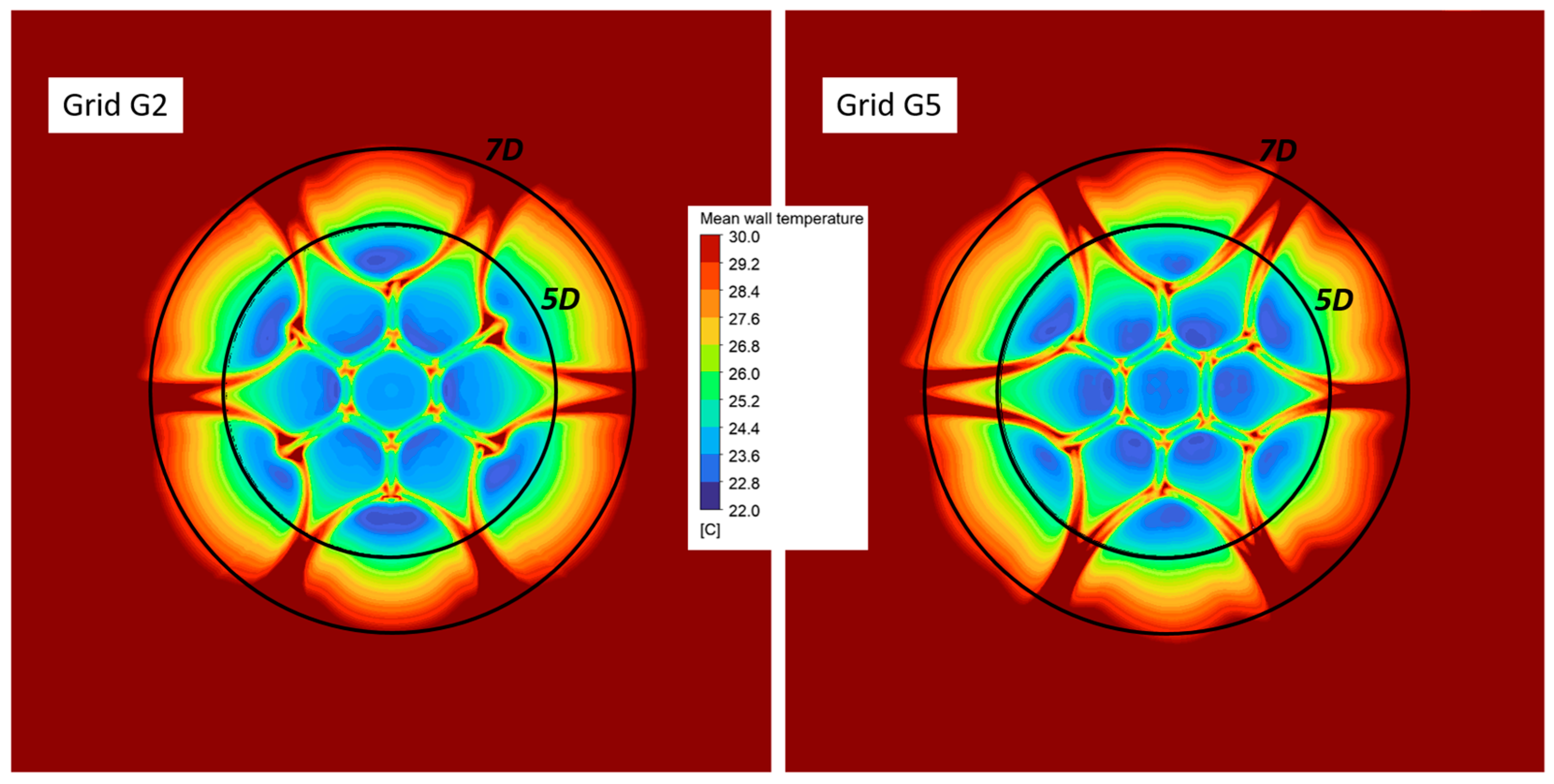
The contours of the mean temperature at the impingement plate (obtained with RANS simulations) are presented in Figure 9. It may be observed that the most effective cooling is achieved in the central region of the configuration, i.e., within a concentric area with a radius of approximately 6 nozzle diameters. It is noted that hot spots (with locally higher wall temperature) occur at locations between jets, where adjacent wall-jets collide and fountain flow is formed. Contrarily, the temperature distribution at the impingement plate from the LES, shown in Figure 10, is more uniform and does not exhibit so pronounced hot spots within the jet configuration. Such, a “smoother” temperature pattern is reasonable for LES since the mean temperature is obtained from instantaneous heat transfer characteristics with time averaging. From the RANS results shown here, it may be observed that the wall temperature patterns exhibit a “weak” asymmetry, which is observed to occur for all tested mesh topologies and resolutions, i.e., for structured hexahedral and unstructured polyhedral meshes.

The results of the current study with five different computational grids are presented in

Table 2. Mean heat transfer characteristics.

	${\mathit{T}}_0^{\mathit{w}}$ [°C]	${\overline{{\mathit{T}}_{\mathbf{w}\mathbf{a}\mathbf{l}\mathbf{l}}}}^{5\mathit{D}}$ [°C]
G1	23.5	24.0
G2	23.8	24.8
G3	23.8	24.7
G4	23.8	24.7
G5	23.3	24.8
LES	23.2	25.0

. The mean wall temperature at the stagnation point $T_{\mathrm{wall}}^0$ is reported together with the area-weighted average temperature of the wall ${\overline{\left(T_{\mathrm{wall}}\right)}}^{5D}$, computed across the circular area, with a diameter $r/D$ equal to five. The LES results are shown for comparison as well.

It is observed that all RANS simulations yield very similar results. The computed mean wall temperature at the stagnation point ($T_{\mathrm{wall}}^0$) is less than 1 °C different from that of the LES. A very good agreement with the LES prediction is also observed for the computed area-weighted average temperature of the wall ${\overline{\left(T_{\mathrm{wall}}\right)}}^{5D}$. From the wall temperature profiles (located far from the plate geometrical center (|r|/D > 3.0)), which are shown in Figure 8, it may be observed that slightly lower wall temperature is predicted by RANS simulations as compared to the LES. On the other hand, smaller differences in predicted wall temperature between RANS simulations and LES are observed in the stagnation region of individual jets. As such, the obtained area-weighted average temperature of the wall ${\left(\overline{T_{\mathrm{wall}}}\right)}^{5D}$is slightly higher from the LES as compared to the RANS computations.

5. Conclusions

This work investigates how the mesh resolution and topology affect the predicted mean flow and heat transfer characteristics of multiple turbulent impinging jets in steady RANS simulations with the SST k-ω turbulence model. The computations are performed with the commercial code ANSYS Fluent R21.2. The results are validated against the existing LES results [4,16] and the experimental data [30,31,32].

This study shows that the mean heat transfer characteristics can be well predicted with the steady-state RANS approach. A sensitivity study with five different computational grids, differing in topology and resolution, has shown that even a coarse grid, with only four cells across jets’ diameter at the half-height of the confinement, is able to adequately predict the local mean flow characteristics near the impingement plate, as long as the near-wall grid spacing is sufficiently small ($y^{+} ~ 1$). The mean wall temperature at the stagnation point ($T_{\mathrm{wall}}^0$), computed by RANS simulations, is less than 1 °C different from that of the LES. A very good agreement with the LES is also observed in the computed area-weighted average temperature of the wall $\left({\overline{\left(T_{\mathrm{wall}}\right)}}^{5D}\right)$, which confirms the potential of the steady-state RANS approach in the assessment of the mean heat transfer characteristics of multiple turbulent impinging jets.

Given the fact that the flow of a single impinging jet is influenced by many factors, such as the nozzle geometry, nozzle-to-plate distance, Reynolds number, etc., the findings from this study to other conditions and geometries of multiple jet arrays are very challenging. For example, Geers et al. [30,31] experimentally observed that, as the nozzle-to-plate distance increases, the imprints of impinging jets at the target plate are displaced radially outward. This phenomenon is attributed to jet-to-jet interactions resulting from colliding wall-jets (formed after impingement) and the effects of self-induced cross-flow, where the fluid from inner jets leaves the configuration. It is speculated that a very similar effect can be expected with an increase in Reynolds number for a given set of geometrical parameters.

Simulations of practical, industry-level applications, typically performed with coarse meshes and statistical turbulence models, cannot realistically replicate the intricate flow dynamics of multiple turbulent impinging jets. Nevertheless, the current study implies that, for reasonably accurate predictions of mean heat transfer characteristics needed for conceptual design studies, the consideration of the latter phenomena might not be essential.

References

1. Weigand, B.; Spring, S. Multiple jet impingement—A review. In TURBINE-09, Proceedings of the International Symposium on Heat Transfer in Gas Turbine Systems, Antalya, Turkey, 9–14 August 2009; Begel House Inc.: Danbury, CT, USA, 2009. [Google Scholar] [CrossRef]
2. Zuckerman, N.; Lior, N. Jet impingement heat transfer: Physics, correlations, and numerical modeling. Adv. Heat Transf. 2006, 39, 565–631. [Google Scholar] [CrossRef]
3. Dewan, A.; Dutta, R.; Srinivasan, B. Recent Trends in Computation of Turbulent Jet Impingement Heat Transfer. Heat Transf. Eng. 2012, 33, 447–460. [Google Scholar] [CrossRef]
4. Draksler, M.; Končar, B.; Cizelj, L.; Ničeno, B. Large Eddy Simulation of multiple impinging jets in hexagonal configuration—Flow dynamics and heat transfer characteristics. Int. J. Heat Mass Transf. 2017, 109, 16–27. [Google Scholar] [CrossRef]
5. Norajitra, P.; Giniyatulin, R.; Ihli, T.; Janeschitz, G.; Krauss, W.; Kruessmann, R.; Kuznetsov, V.; Mazul, I.; Widak, V.; Ovchinnikov, I.; et al. He-cooled divertor development for DEMO. Fusion Eng. Des. 2007, 82, 2740–2744. [Google Scholar] [CrossRef]
6. The Demonstration Power Plant: DEMO. Available online: https://www.euro-fusion.org/programme/demo/ (accessed on 20 December 2023).
7. Le Song, G.; Prud’homme, M. Prediction of coherent vortices in an impinging jet with unsteady averaging and a simple turbulent model. Int. J. Heat Fluid Flow 2007, 28, 1125–1135. [Google Scholar] [CrossRef]
8. Rao, G.A.; Kitron-Belinkov, M.; Levy, Y. Numerical analysis of a multiple jet impingement system. In Proceedings of the ASME Turbo Expo 2009: Power for Land, Sea, and Air, Orlando, FL, USA, 8–12 June 2009; Volume 48845, pp. 629–639. [Google Scholar] [CrossRef]
9. Zu, Y.Q.; Yan, Y.Y.; Maltson, J.D. CFD prediction for multi-jet impingement heat transfer. In Proceedings of the ASME Turbo Expo 2009: Power for Land, Sea, and Air, Orlando, FL, USA, 8–12 June 2009; Volume 48845, pp. 483–490. [Google Scholar] [CrossRef]
10. Webb-Martin, S.; Yang, Z. Assessment of Urans approach for predicting twin impinging jets in a cross-flow. In Proceedings of the 9th International Conference on Heat Transfer, Fluid Mechanics and Thermodynamics, St. Julian’s, Malta, 16–18 July 2012; Available online: http://hdl.handle.net/2263/44776 (accessed on 20 December 2023).
11. Khayrullina, A.; van Hooff, T.; Blocken, B.; van Heijst, G. Validation of steady RANS modelling of isothermal plane turbulent impinging jets at moderate Reynolds numbers. Eur. J. Mech.-B/Fluids 2019, 75, 228–243. [Google Scholar] [CrossRef]
12. Menter, F. Zonal Two Equation kw Turbulence Models For Aerodynamic Flows. In Proceedings of the 23rd Fluid Dynamics, Plasmadynamics, and Lasers Conference, Orlando, FL, USA, 6–9 July 1993; p. 2906. [Google Scholar] [CrossRef]
13. Menter, F.; Egorov, Y. A scale adaptive simulation model using two-equation models. In Proceedings of the 43rd AIAA Aerospace Sciences Meeting and Exhibit, Reno, NV, USA, 10–13 January 2005; p. 1095. [Google Scholar] [CrossRef]
14. Bovo, M.; Davidson, L. On the transient modelling of impinging jets heat transfer. A practical approach. In THMT-12, Proceedings of the Seventh International Symposium on Turbulence Heat and Mass Transfer, Palermo, Italy, 24–27 September 2012; Begel House Inc.: Danbury, CT, USA, 2012. [Google Scholar] [CrossRef]
15. Draksler, M.; Tekavčič, M.; Končar, B. Simulation of heat transfer in multiple impinging jets with scale-adaptive turbulence model. In Proceedings of the 30th International Conference Nuclear Energy for New Europe—NENE 2021, Bled, Slovenia, 6–9 September 2021; Nuclear Society of Slovenia: Ljubljana, Slovenia, 2021; pp. 621.1–621.8. [Google Scholar]
16. Draksler, M.; Končar, B.; Cizelj, L. On the accuracy of Large Eddy Simulation of multiple impinging jets. Int. J. Heat Mass Transf. 2019, 133, 596–605. [Google Scholar] [CrossRef]
17. Yang, Z. Assessment of unsteady-RANS approach against steady-RANS approach for predicting twin impinging jets in a cross-flow. Cogent Eng. 2014, 1, 936995. [Google Scholar] [CrossRef]
18. Barata, B.A.C.; Navalho, J.E.P.; Pereira, J.C.F. Prediction of Self-Sustained Oscillations of an Isothermal Impinging Slot Jet. Fluids 2023, 8, 15. [Google Scholar] [CrossRef]
19. Martínez-Filgueira, P.; Portal-Porras, K.; Fernandez-Gamiz, U.; Zulueta, E.; Soriano, J. Experimental and numerical modeling of an air jet impingement system. Eur. J. Mech. B Fluids 2022, 94, 228–245. [Google Scholar] [CrossRef]
20. Kubacki, S.; Dick, E. Hybrid RANS/LES of flow and heat transfer in round impinging jets. Int. J. Heat Fluid Flow 2011, 32, 631–651. [Google Scholar] [CrossRef]
21. Wu, W.; Piomelli, U. Reynolds-averaged and wall-modelled large-eddy simulations of impinging jets with embedded azimuthal vortices. Eur. J. Mech. B Fluids 2016, 55, 348–359. [Google Scholar] [CrossRef]
22. Esch, T.; Menter, F. Heat transfer predictions based on two-equation turbulence models with advanced wall treatment. Turbulence. Heat Mass Transf. 2003, 4, 633–640. [Google Scholar]
23. Behnia, M.; Parneix, S.; Durbin, P. Prediction of heat transfer in an axisymmetric turbulent jet impinging on a flat plate. Int. J. Heat Mass Transf. 1998, 41, 1845–1855. [Google Scholar] [CrossRef]
24. Behnia, M.; Parneix, S.; Shabany, Y.; Durbin, P. Numerical study of turbulent heat transfer in confined and unconfined impinging jets. Int. J. Heat Fluid Flow 1999, 20, 1–9. [Google Scholar] [CrossRef]
25. Wei, T.; Oprins, H.; Cherman, V.; Beyne, E.; Baelmans, M. Conjugate Heat Transfer and Fluid Flow Modeling for Liquid Microjet Impingement Cooling with Alternating Feeding and Draining Channels. Fluids 2019, 4, 145. [Google Scholar] [CrossRef]
26. Maddox, J.F. Liquid Jet Impingement with Spent Flow Management for Power Electronics Cooling. Ph.D. Thesis, Auburn University, Auburn, AL, USA, 2015. [Google Scholar]
27. Gurgul, S.; Fornalik-Wajs, E. On the Measure of the Heat Transfer Performance of RANS Turbulence Models in Single Round Jet Impingement. Energies 2023, 16, 7236. [Google Scholar] [CrossRef]
28. Menter, F.R.; Lechner, R.; Matyushenko, A. Best Practice: RANS Turbulence Modeling in Ansys CFD; Version 1.0; ANSYS, Inc.: Canonsburg, PA, USA, 2021. [Google Scholar]
29. V2F Turbulent Model in FLUENT. Available online: https://forum.ansys.com/forums/topic/v2f-turbulent-model-in-fluent/ (accessed on 17 November 2023).
30. Geers, L.F.G.; Tummers, M.J.; Hanjalic, K. Experimental investigation of impinging jet arrays. Exp. Fluids 2004, 36, 946–958. [Google Scholar] [CrossRef]
31. Geers, L.F.G.; Tummers, M.J.; Hanjalić, K. Particle imaging velocimetry-based identification of coherent structures in normally impinging multiple jets. Phys. Fluids 2005, 17, 055105. [Google Scholar] [CrossRef]
32. Geers, L.F. Multiple Impinging Jet Arrays: An Experimental Study on Flow and Heat Transfer. Ph.D. Thesis, Delft University of Technology, Delft, The Netherlands, 2003. [Google Scholar]
33. ANSYS, Inc. Fluent Theory Guide, ANSYS® Academic Research, Release 2021R2; ANSYS, Inc.: Canonsburg, PA, USA, 2021. [Google Scholar]
34. PSI-BOIL Webpage. Available online: https://www.psi.ch/en/lsm/psi-boil (accessed on 20 December 2023).
35. Nicoud, F.; Ducros, F. Subgrid-Scale Stress Modelling Based on the Square of the Velocity Gradient Tensor. Flow Turbul. Combust. 1999, 62, 183–200. [Google Scholar] [CrossRef]
36. ANSYS, Inc. Fluent Users Guide, ANSYS® Academic Research, Release 2021R2; ANSYS, Inc.: Canonsburg, PA, USA, 2021. [Google Scholar]
37. Langley Research Center. Turbulence Modeling Resource. The Menter Shear Stress Transport Turbulence Model. Available online: https://turbmodels.larc.nasa.gov/sst.html (accessed on 20 November 2023).
38. Zore, K.; Azab, M.; Sasanapuri, B.; Shah, S.; Stokes, J. ANSYS scale resolving simulations of launch-vehicle configuration at transonic speeds. In Proceedings of the 21st AeSi Annual CFD Symposium, Bengaluru, India, 8–9 August 2019; pp. 8–9. [Google Scholar]
39. Draksler, M.; Končar, B. Analysis of heat transfer and flow characteristics in turbulent impinging jet. Nucl. Eng. Des. 2011, 241, 1248–1254. [Google Scholar] [CrossRef]
40. Kato, K. The modeling of turbulent flow around stationary and vibrating square cylinders. In Proceedings of the of 9th Symposium on Turbulent Shear Flows, Kyoto, Japan, 16–18 August 1993; pp. 1041–1046. [Google Scholar]
41. ANSYS, Inc. Meshing, ANSYS® Academic Research, Release 2021R2; ANSYS, Inc.: Canonsburg, PA, USA, 2021. [Google Scholar]
Figure 1. Schematics of the experimental test section indicating the region of interest where measurements were taken.
Energies 17 00196 g001
Figure 2. Simulation domain with characteristic cross-section planes P-1 and P-2, where numerical results are presented.
Energies 17 00196 g002
Figure 3. Grid topology at the nozzle plate. (Left): grid G2; (Right): grid G5.
Energies 17 00196 g003
Figure 4. Vertical cross-section of the grid. (Left): grid G2; (Right): grid G5.
Energies 17 00196 g004
Figure 5. Mean axial velocity V / V c l profiles in plane P-1 (left) and in plate P-2 (right). Symbols indicate the experimental results by Geers et al. [30,32].
Energies 17 00196 g005
Figure 6. Mean turbulence kinetic energy k / V c l 2 profiles in plane P-1 (left) and in plate P-2 (right). Symbols indicate the experimental results by Geers et al. [30,32].
Energies 17 00196 g006
Figure 7. Contours of mean axial velocity V / V c l (left) and mean turbulence kinetic energy k / V c l 2 (right) in plane P-1. Red vertical lines indicate the geometrical axes of individual jets.
Energies 17 00196 g007
Figure 8. Horizontal profiles of mean flow characteristics and mean wall temperature T wall . Mean axial velocity V / V c l , normalized mean eddy viscosity ν t / ν , and mean turbulence kinetic energy k / V c l 2 are extracted at y / D = 0.0125 above the impingement surface. (Left): Plane P-1; (Right): Plane P-2. Symbols indicate the experimental results by Geers [32].
Energies 17 00196 g008
Figure 9. Contours of the mean temperature at the impingement plate. (Left): grid G2; (Right): grid G5.
Energies 17 00196 g009
Figure 10. Contours of the mean temperature at the impingement plate from LES.
Energies 17 00196 g010