Modelling Energy Data in a Generalized Additive Model—A Case Study of Colombia

Abstract

Energy demand modelling is essential for reliable informing and framing energy policy decisions. More accurate modelling betters ensuring availability of energy and energy quality. Energy availability is related to energy access across the country and defines important economic measures such as energy poverty, which plays a critical role in developing countries. Energy quality is related to the reliability of the supply for correctly estimating energy needs. To incorporate spatial and temporal components of energy in a way that availability and quality are accurately assessed, this article discussed a number of suitable task methods for this (Second-generation GAMs with one-dimensional smoothers: Cyclic/Non-Cyclic Cubic Splines and two-dimensional smoothers: Markov Random Fields/Tensor Splines Interactions). The results showed that the complete consideration of both temporal and spatial aspects leads to a better fitted model which explains more of the data variation.

1. Introduction

Energy demand modelling in developing countries plays a huge role in framing policy decisions for energy management, as a country’s rapid pace of transformation calls for models that both adjust to short-term needs but also for more refined approaches that allow to make long-term plans for energy coverage. In that sense, quantitative analyses that evaluate a country’s population energy consumption across time and space are important because they enable the identification of gaps in energy access and patterns in energy consumption avoiding underestimation-shortage and overestimation-costs.

Ensuring access to affordable, reliable, sustainable, and modern energy is the seventh goal in the sustainable development goals from the United Nations [1]. Unfortunately, this has been hard to accomplish for Colombia due to the geography of the country with a considerable amount of land, around a million square kilometers, equivalent to three medium-sized European countries. In addition to, natural barriers such as mountains or rivers create connectivity difficulties and lead to elevated costs of energy installations [2].

The vulnerability of the poor is aggravated by climate change and the volatility of energy prices [3]. For tropical countries such as Colombia, those two aspects are strongly associated with temporal demand variation. On one side, climate change makes the rainy/dry season more pronounced and aggressive, which can be addressed in a model by including a yearly pattern. On the other side, the volatility of energy prices is hard to control if no modelling is implemented over energy data and if the tendencies and patterns are unknown.

Often the spatial aspect is ignored when modelling energy [4], meaning that neither consulting companies nor governmental entities, especially in developing countries, include spatial elements in energy modelling. Nonetheless, the spatial characteristics of the data when modelled can explain a lot about what is happening in the regions and can often be linked to socio-economic characteristics (i.e., size or number of households) of the regions. Analyses using global data sets or global analyses often fail to provide sufficient information on energy access [3].

To date, the spatial information in Colombia that is publicly accessible in regards to energy is given by the energy operators, which can be associated with regions, but there is not further detail available publicly related to households. Each energy operator has its separate household information, but this information is being sent already aggregated to the government entities that foresee the energy market. Therefore, there is no way of desegregating the data at a further level of detail.

In 2007, four percent of the Colombian population was not connected to the national grid accounting for sixty-six percent of the national territory [5]. Since then there has not been any other publication that addresses the percentage of the population that dwells in the non interconnected energy grid areas, this could nevertheless be inferred from the reports of non-interconnected zones/departments plus census data. In 2014 a map of non-interconnected zones showed that eleven out of the thirty-two departments were partially or entirely not connected to the grid [2] (See Figure 1). This is equivalent to fifty-four percent of the territory when measured by department area. An analysis over historical demand in 2018 unveiled that five out of thirty-two departments were not connected to the national grid which is equivalent to thirty percent of the territory when measured by department area [6]. Even with an improvement of twenty percent on energy coverage between the years 2014 and 2018 there is still a significant portion of the country that is not being accounted for.

Scarcity in energy access or availability is common in developing countries, inherently related to space rather than time makes modelling exclusively with temporal parameters not ideal. Broadening the access to modern energy services is something that needs to be addressed by all countries but also represents a colossal challenge for the developing ones [3].

This article explores the potential of combining spatial and temporal data for improving the reliability of energy demand modelling in Colombia with the constraints data available to date has while stating modelling possibilities for future data desegregated at a lower level.

2. Materials and Methods

This article explores the use of second Generation GAMs to model spatial-temporal energy data with one-dimensional smoothers: Cubic Splines Cyclic and Non-Cyclic, and two-dimensional smoothers: Markov Random Fields and Tensor Splines, for the interactions used as case study data from Colombia. Smoothing splines through GAMs are more flexible than classically used GLMs, recognizing and characterizing non-linear relationships that can accommodate both space and time covariates [7]. Gaussian Markov Random Fields as Penalized Regression Spline make use of the penalty precision matrix to fit the smoothers to the data.

2.1. One Dimensional Smoothers: Cubic Regression Splines Non-Cyclic and Cyclic

A commonly used method for modelling time in energy demand modelling is the Cubic Regression Spline due to its high interpretability [8]. Cubic splines are widely used in the literature to model non-linear relationships not only in the energy field but also in other fields as well [9,10]. Splines of degree df are defined as a continuous piecewise polynomial $b_1\left(x\right),b_2\left(x\right),\dots ,b_k\left(x\right)$ of the same degree with k basis functions, also called knots at ${ϵ}_1,\dots ,{ϵ}_k$ regions of the explanatory variable x [11].

According to Ref. [8] a spline can be represented as

$$f\left(x\right)=\sum _{j=1}^k{b}_j\left(x\right){\gamma }_j$$

(1)

where $b_j$ are the basis functions and ${\gamma }_j$ is the vector containing all the basis coefficients. Ref. [10] reframes Equation (1) based on not just the knots k but also the degree of the spline $df$ as

$$f\left(x\right)=\sum _{k=1}^{K+df+1}{b}_k\left(x\right){\gamma }_k$$

(2)

The idea of this is that with k knots there are $k+1$ polynomials of degree $df$, which makes the model have $k\ast df$ constraints, which generates $(k+1)(df+1)-k\ast df=k+df+1$ free parameters as pointed out by Ref. [10]. In a cubic spline the degrees of freedom are therefore $k+4$.

The representation of a cyclic spline is the same as for a cubic one, with the exception being that the limits of the summation do not go until the k, but until $k-1$ due to the cyclic end condition

$$f\left(x\right)=\sum _{j=1}^{k-1}\widetilde{b_j}\left(x\right){\gamma }_j$$

(3)

Both cubic and cyclic spline have a second derivative that follows

$$J\left(x\right)={\int }_{x_1}^{x_k}{f}^{″}{\left(x\right)}^{2}dx$$

(4)

Equation (4) is equivalent to ${\gamma }^T{D}^T{B}^{-1}D\gamma$ if the spline is cubic and ${\gamma }^T{\tilde{D}}^T{\tilde{B}}^{-1}\tilde{D}\gamma$ if the spline is cyclic cubic and they both can be summarized into ${\gamma }^{T}S\gamma$ and ${\gamma }^T\tilde{S}\gamma$, where S and $\tilde{S}$ are the penalty matrices for each cubic and cyclic cubic spline, respectively.

2.2. Two Dimensional Smoother: Tensor Product Smooth Interactions

All the concepts referred to in this section are derived from Ref. [8].

In order to include the interaction between the one-dimensional smoother, a tensor product smooth interaction was included. If there are two covariates x and z with smooth functions $f\left(x\right)$ and $f\left(z\right)$ with basis $b_j\left(x\right)$ and $a_m\left(z\right)$ such as

$$f\left(x\right)=\sum _{j=1}^k{b}_j\left(x\right){\gamma }_{j}andf\left(z\right)=\sum _{m=1}^l{a}_m\left(z\right){\delta }_m$$

(5)

Therefore, the smooth function of $f(x,z)$ can be represented as

$$f(x,z)=\sum _{j=1}^k\sum _{m=1}^l{b}_j\left(x\right)a_m\left(z\right){\delta }_{jm}$$

(6)

This assumes that the vector containing the basis coefficients for x${\gamma }_j$ varies smoothly with z such as

$${\gamma }_j\left(z\right)=\sum _{m=1}^l{a}_m\left(z\right){\delta }_{jm}$$

(7)

The tensor product penalties are also derived from the associated penalty function for each covariate

$$J\left(x\right)={\gamma }^T{S}_x\gamma andJ\left(z\right)={\delta }^T{S}_z\delta$$

(8)

leading to a double penalty based on the tensor product of Equation (8) such as

$$J_x\left(f(x,z)\right)={\gamma }^T\overline{S_x}\gamma and{J}_z\left(f(x,z)\right)={\gamma }^T\overline{S_z}\gamma$$

(9)

where $\gamma$ is the vector of ${\gamma }_{jl}$ arranged in the corresponding order according to covariates x and z, $\overline{S_x}$ is the marginal penalty matrix for x and $\overline{S_z}$ is the marginal penalty matrix for z.

2.3. Two Dimensional Smoother: Markov Random Fields

In a space where two-dimensional smoothers have to be used, Markov random fields can be fitted through a neighbourhood structure that works well with discrete geographic regions. As stated by Ref. [12] a random field, also called a stochastic field, is a collection of random variables $X\left(s\right)=X\left(s_1\right),X\left(s_2\right),\dots ,X\left(s_n\right)$ at locations $s_1,s_2,\dots ,s_n$$s\in R^n$ where each random variable is defined on a probability space $(\Omega ,F,P)$ where $\Omega$ is an abstract sample space also known as topological space, F is a field of subsets of the abstract sample space $\Omega$ and P is the probability measure on the space $(\Omega ,F)$ that satisfies the Kolmogorov axioms: (a) $P(\Omega )=1$, (b) $0<P\left(A_i\right)<1$ for all sets $A_i\in F$ and (c) If $A_i\in F$ and $A_i\cap A_j=⌀$ then $P({\bigcup }_{i=1}^{\infty }{A}_i={\sum }_{i=1}^{\infty }P\left(A_i\right)$.

The random fields range from Gaussian to Non-Gaussian and from Discrete to Continuous [12] and can be applied over space or time [13]. For this application over discrete space lattice or areal regionally aggregated data, Gaussian random fields were preferred for being more intuitive when compared with non-Gaussian ones [14]. A Gaussian Random Field (GMRF), as defined by Ref. [15], is a random vector of n finite dimensions $X\left(s\right)=X\left(s_1\right),X\left(s_2\right),\dots ,X\left(s_n\right)$ for a finite set of locations $s_1,s_2,\dots ,s_n$$s\in R^n$ that follows a multivariate Gaussian/Normal distribution $XN(\mu ,\Sigma )$ with mean vector $\mu$ and positive definite covariance matrix $\Sigma$ such as

$$\mu =E\left[X\left(s\right)\right]=\left(\begin{array}{c}E\left(X\left(s_1\right)\right)\\ E\left(X\left(s_2\right)\right)\\ \cdots \\ E\left(X\left(s_n\right)\right)\end{array}\right)$$

(10)

$$\Sigma =Cov(X\left(s_i\right),X\left(s_j\right))$$

$$\begin{array}{c}\hfill \left(\begin{array}{cccc}Cov(X\left(s_1\right),X\left(s_1\right))& Cov(X\left(s_1\right),X\left(s_2\right))& \cdots & Cov(X\left(s_1\right),X\left(s_n\right))\\ Cov(X\left(s_2\right),X\left(s_1\right))& Cov(X\left(s_2\right),X\left(s_2\right))& \cdots & Cov(X\left(s_2\right),X\left(s_n\right))\\ \cdots & \cdots & \cdots & \cdots \\ Cov(X\left(s_n\right),X\left(s_1\right))& Cov(X\left(s_n\right),X\left(s_2\right))& \cdots & Cov(X\left(s_1\right),X\left(s_n\right))\end{array}\right)\end{array}$$

(11)

The multivariate normal distribution for the random vector $X\left(s\right)$ of n finite dimensions with the mean vector $\mu$ and covariance matrix $\Sigma$ is the following

$$p\left(X\right)=\frac{{\Sigma }^{-1/2}}{2{\pi }^{n/2}}exp\left\{-\frac{1}{2}{(X-\mu )}^T{\Sigma }^{-1}(X-\mu )\right\}$$

(12)

The Gaussian Random Field (GMRF) can also be defined in terms of a sparse matrix allowing the employment of sparse matrix solution techniques and properties and ultimately a faster computation, as indicated by Ref. [15]. The precision sparse matrix, in this case would be the inverse of the covariance matrix such as $Q={\Sigma }^{-1}$, making the model become $XN(\mu ,Q^{-1})$. The multivariate Normal distribution for the random vector $X\left(s\right)$ of n finite dimensions when using the precision sparse matrix Q instead of the covariance matrix $\Sigma$ could be expressed as

$$p\left(x\right)=\frac{{\left|Q\right|}^{1/2}}{2{\pi }^{n/2}}exp\{-\frac{1}{2}{(X-\mu )}^{T}Q(X-\mu )\}$$

(13)

This finite set of locations $s_1,s_2,\dots ,s_n$$S\in R^n$ from the Gaussian Random Field (GMRF) are defined within a neighbourhood structure that is represented through an undirected labelled graph $g=(v,ϵ)$ where v is a set of labelled nodes/regions $v=1,\dots ,n$ and $ϵ$ is a set of undirected edges from node i to node j $i,j$ where $i,j\in v$ and $i\ne j$ n the case of areal data the edges are the spatial borders between the regions.

If the regions share a common border, then the sparse matrix is non-zero $Q_{ij}\ne 0$ and the regions i and j are neighbours such as $ne\left(i\right)=j⟺ne\left(j\right)=i$, which can also be expressed as $i\sim j⟺j\sim i$. It can be said that the neighbouring regions i and j are conditionally dependent such as $p\left(x_i\right|x_j)$ when $i,j\in vandi\ne j$.

If regions i and j do not share any spatial border, then there is no edge between i and j, and then the sparse matrix is zero $Q_{ij}=0$, and that $x_i\perp x_j|x_{-ij}$ for all $i\ne j$, which means that the regions i and j are not neighbours and are conditionally independent of all the other regions in the neighbourhood structure, and $x_{-ij}$ indicates all elements except for i and j.

For the case presented here, a fully connected neighbourhood structure is assumed, which can be represented through a fully connected undirected labelled graph, in which $i,j\in ϵ$ for all $i,j\in v$ with $i\ne j$.

Figure 2 represents an areal data neighbourhood structure with 14 nodes or regions such as $v=\{0,1,2,3,4,5,6,7,8,10,11,12,13,14\}$ and with 29 as the set of edges or boundaries between regions

$$ϵ=\left\{\begin{array}{cccc}\{7,13\},& \{7,2\},& \{13,2\},& \{13,11\},\\ \{13,3\},& \{13,6\},& \{2,12\},& \{2,11\}\\ \{12,11\},& \{12,8\},& \{11,8\},& \{11,0\}\\ \{11,3\},& \{8,0\},& \{8,1\},& \{6,14\}\\ \{10,14\},& \{10,4\},& \{14,4\},& \{4,5\}\\ \{5,1\}\end{array}\right\}$$

As can be seen in Figure 2, region 7 is a neighbour of regions 2 and 13 such as $nei\left(7\right)=\{2,13\}$, region 13 has as neighbours the regions 7, 2, 11, 3, and 6 such as $nei\left(13\right)=\{7,2,11,3,6\}$, and so on. The average amount of neighbours for this neighbourhood structure is four, with a minimum of two neighbours in region 7 and a maximum of seven neighbours in region 0, such as $nei\left(0\right)=\{11,8,3,14,4,5,1\}$.

3. Results

The demand data in this study is kilowatts hourly information collected monthly and published yearly by the entity that oversees the grid of the electricity sector in Colombia [6] (See Figure 3).

The input data used for both spatial and temporal regressions are hourly aggregated information for each department by day in a range of five years from 2013 to 2018. No disaggregated information from smaller administrative areal units such as municipalities or point data about home consumption was available. The thirty-two departments were grouped into fifteen regions for this analysis, as shown in

Table A1. Grouping of states into regions.

Region	State
Costa Atlantica	La Guajira
	Magdalena
	Atlántico
	Cesar
	Bolívar
	Sucre
	Córdoba
Oriente	Norte de Santander
	Santander
	Boyacá
	Arauca
	Casanare
Antioquia	Antioquia
Chocó	Chocó
CQR	Caldas
	Risaralda
	Quindío
Valle	Valle del Cauca
Sur	Cauca
	Nariño
	Putumayo
Centro	Cundinamarca
	Bogotá
	Meta
Guaviare	Guaviare
THC	Tolima
	Huila
	Caquetá
Amazonas	Amazonas
Vaupés	Vaupés
Guainía	Guainía
Vichada	Vichada

from Appendix A.

3.1. Non-Spatial GAM: Generalized Additive Model Regression Using Cubic Splines as a One-Dimensional Smoother for Modelling Time

Additive models were introduced by Ref. [16] to deal with the dimensionality problem of the General Linear Models GLMs through univariate smoothing [17]. The GAMs Stone approach can be seen as a traditional way of portraying GAMs, which in this case has the demand as the response variable d, and space or time as predictors $x_j$, which can be written as

$$d={\alpha }_0+f_1\left(x_1\right)+f_2\left(x_2\right)+\cdots +f_k\left(x_k\right)+ϵ$$

(14)

or its summarised version

$$d={\alpha }_0+\sum _{j=1}^k{f}_j\left(x_j\right)+ϵ$$

(15)

where ${\alpha }_0=E\left[f\left(x\right)\right]$ and $f_j$ are the smooth functions over the covariates $x_j$.

The Stone approach fails to include interaction and therefore has unsatisfactory results when interaction exists [18]. It is here that the approach from Ref. [11] becomes important, as it not only includes interactions $f_j$ but also includes the link function g over the response variable d to analyse $x_j$ within a solution space of any member of the exponential family, usually Gaussian-Normal, but it is open to Gamma, Poisson, or Binomial [17]. Then, a Generalized Additive model over the demand according to the Hastie and Tibshirani approach can be written as

$$g\left(\mu \right)=\alpha +\sum _{j=1}^k{f}_j\left(x_j\right)+ϵ$$

(16)

where $f_j$ are the smooth functions over the covariates $x_j$ allowing for both single basis smoothing ${\sum }_j{f}_j\left(x_j\right)$ and interactions ${\sum }_{j\ne i}{f}_j(x_i,x_j)$ and $\mu =E\left(d\right)$. In this approach, $\alpha$ is a regression for the variables that will not be modelled additively. Hastie and Tibshirani defineed the procedure for estimating $\alpha$ and $f_j$ as a local scoring procedure for generalized additive models.

In the early 2000s, Ref. [19] provided a more recent perspective to the GAM definition developed by Ref. [11], denoted in Equation (13). The author directly defined the iterative procedure with a model structure that has index i, in which $\alpha$ is represented as the product of the model matrix A and a vector of the associated model parameters $\theta$, where the intercept is assumed to be included. A is a design matrix for the covariates x with linear effects. The author also included a linear operator $L_{i}j$ to multiply the smooth function $f_j$.

$$g\left({\mu }_i\right)=A_i\theta +\sum _{j=1}^k{L}_{ij}{f}_j\left(x_j\right)+{ϵ}_i$$

(17)

where $d_i$ is distributed according to an exponential family EF that has median ${\mu }_i$ and variance $\varphi$, $d_i\sim EF({\mu }_i,\varphi )$.

The cubic regression spline smoother is represented through the function $f_j$ where $b_j$ is a base function of the spline and ${\gamma }_j$ is the vector containing all the basis coefficients such as

$$f_j\left(x_j\right)=\sum _{j=1}^k{b}_j\left(x\right){\gamma }_j$$

(18)

Finally, a vector of coefficients $\gamma$ that contains the linear fixed effects vector $\theta$ followed by all the basis coefficients $\gamma$ for $f_j$ such as $\gamma =\{\theta ,{\gamma }_1,\dots ,{\gamma }_k\}$ is defined. Then the estimation of the vector of coefficients $\widehat{\gamma }$ from the GAM model will be done by penalized maximum likelihood, where the optimal is given by some smoothing parameters ${\delta }_j$ [19]

$$\hat{\gamma }=argmi{n}_{\gamma }\left(D\left(\gamma \right)+\sum _{j=1}^k{\delta }_j{\gamma }^T{S}_j\gamma \right)$$

(19)

where $S_j$ is a penalty matrix and the deviance of the model $D\left(\gamma \right)=2(l\left({\gamma }_{m}ax\right)-l\left(\gamma \right))\varphi$.

Note that not only the optimal vector of coefficients $\hat{\gamma }$ must be estimated but also the parameters themselves ${\delta }_j$. The smoothing parameters estimation ${\delta }_j$ is done either by prediction error criteria (GCV) or maximum likelihood (ML or REML) [20].

The method that we will be used in this article for selecting the smoothing parameters ${\gamma }_j$ is the Restricted Maximum Likelihood, REML. This will be done instead of other smoothness selection methods such as ML, Maximum Likelihood, and GCV, Generalized Cross-validation. In REML unlike ML, the estimation of variance components is better, as it has a higher probability of providing a complete rank of estimates of the variance components [21]. On the other hand, REML is preferred over GCV due to it having a higher penalty for overfitting and being less likely to have multiple minimum points, therefore being less likely to have highly variable smoothing parameters ${\lambda }_j$ [22].

In the literature, demand electricity is usually modelled by three patterns: daily, weekly, and monthly. Ref. [4] modelled the previously mentioned patterns through a GAM by preselecting the knots according to the number of unique values of the variables included in the model. In that case, when modelling the patterns, only continuous variables were included with 24 knots for the daily pattern, 7 knots for the weekly pattern, and 12 knots for the monthly pattern. In this case, the daily pattern was included in the model through an hour variable, the weekly pattern through a categorical variable that differentiates days between weekend and weekdays, and instead of including a monthly pattern a trend pattern was included. In the model, the interactions between categorical and numerical variables were included. Knots were not set up based on unique values but on sensible values according to the underlying data.

Initially, the daily pattern was included in the model using a cyclic spline smooth over the discrete variable hour with a range from 0 to 23, $s(hr,bs=cc,k=24)$. After this, the weekly pattern was included in the model as a categorical variable, wk, where weekly days were classified as 1-Monday and 7-Sunday, and were aggregated into two factors, $wk/wknd$. The corresponding interaction between the discrete numerical variable that accounts for the daily pattern, hr, and the categorical variable, wk, that accounts for the weekly pattern was also included using a factor smooth-interaction with the argument inside the smooth function, s, in the following way $s(hr,bs=cc,by=wk,k=24)$. Finally, trend pattern was fitted not by using the month’s numeric notation from 1 to 12 or the days of the year from 1 to 365, but through a trend variable that goes from 1 to 43,800, that accounts for the total number of data points available days per years per hour between 2013 and 2018 through a cubic spline smooth $s(time,bs=cr,k=10)$. The interaction between the daily pattern and the trend pattern was fitted using pairwise bivariate tensors product interactions $ti(hr,time,bs=c(cc,cr),k=c(24,10\left)\right)$.

This model can be expressed as

$$\begin{array}{c}\hfill g\left({\mu }_i\right)=A_i+f_1^s\left(hour\right)+weekday+f_3^T\left(time\right)\\ \hfill +f_{1,2}^I\left(hourbyweekday\right)+f_{1,3}^I(hour,time)\end{array}$$

(20)

where $A_i\theta$ accounts for the linear effects and the f function accounts for the non-linear effects defined by each smoothed covariate. The super indexes $S,TandI$ correspond respectively to the Seasonal, Trend, and Interaction components. In the model ${\mu }_i=E\left(d_i\right)$ with the response variable demand being distributed as $d_{i}N({\mu }_i,\varphi )$.

As can be seen in

Table 1. Model summary table for non-spatial GAM.

Rsq	Dev	REML	Scale Est	n
0.852	0.853	$7.573\times {10}^5$	$1.874\times {10}^{11}$	52,584

, the resultant temporal model accounts for eighty-five percent of the electricity demand variation.

The Wald t-test in

Table 2. Parametric coefficients for non-spatial GAM.

Var	Estimate	Std.Error	t-Value	Pr
Intercept	7,146,219	10,848	658.8	$<2\times {10}^{-16}$
weekday (wk/wknd)	−697,836	4180	−166.9	$<2\times {10}^{-16}$

and

Table 3. Smooth terms/non-parametric coefficients for non-spatial GAM.

Var	Estimate	Std. Error	t-Value	Pr
hour-s(hr)	21.2287	22.000	56.312	$<2\times {10}^{-16}$
hour by weekday-s(hr):wk/wk	18.5862	22.000	12.482	$<2\times {10}^{-16}$
hour by weekday-s(hr):wk/wknd	0.6319	22.000	0.029	$7.63\times {10}^{-15}$
time-s(time)	8.8768	8.981	142.593	$<2\times {10}^{-16}$
inter hour and time-ti(hr,time)	90.1125	198.000	4.785	$<2\times {10}^{-16}$

for the non-spatial GAM model shows that all smooth terms and parametric terms are highly significant.

The knots were preselected, but not based on unique values, as in Ref. [4], but on sensible values that reduce the heteroscedasticity of the data as much as possible while maintaining them at logical levels below 24 knots. Splines over 10 knots are rare and can lead to model overfitting, so in this case the upper limit was set to 24 because of the number of unique values of the variable hours. Previous literature also points out that selecting unique values for time related variables makes a better fit.

Heteroscedasticity which indicates if the basis dimension k is too low, was checked through the k-index in

Table 4. K-check for non-spatial GAM.

Var	k	edf	k-Index	p-Value
s(hr)	22	21.2287	0.9827	0.1175
s(hr):wk/wk	22	18.5861	0.9827	0.1075
s(hr):wk/wknd	22	0.6318	0.9827	0.1050
s(time)	9	8.8768	0.8344	0.0000
ti(hr,time)	198	90.1124	0.8369	0.0000

. The model was divided between the residual variance to get a p-value.

The hours variable and its respective interactions showed no evidence of heteroscedasticity with a p-value over zero. On the other hand, the number of data points was clearly heteroscedastic with a p-value around zero. 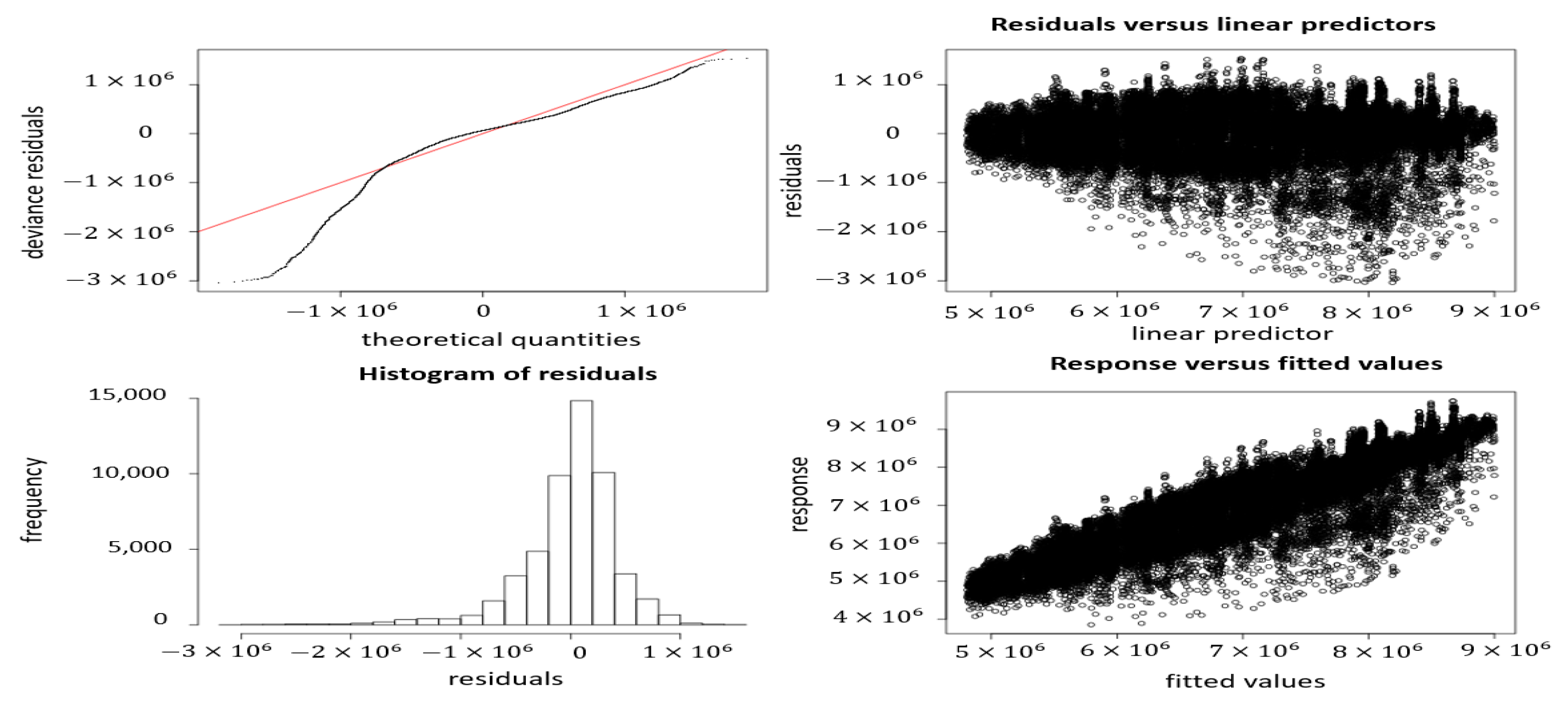For reducing heteroscedasticity in the model, it was attempted to increase the number of knots for the data points variable up to 50, but this had little to no effect in the k-index or p-value. Fifty knots were chosen as an upper limit to test the heteroscedasticity values due to it accounts of two years of data. Going above this value was not explored because the size of the data does not call for a high number of knots, considering that there were only five years available. The residual vs. fitted plot (See Figure 4—second plot from left to right) also shows proofs of heteroscedasticity or non-constant spread in the data.

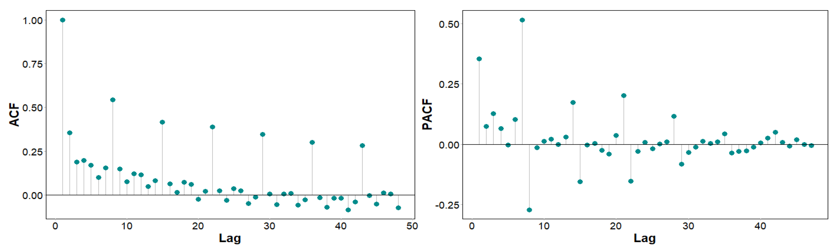
The model demonstrated convergence after ten iterations supporting the data being enough for the number of parameters. However, by looking at the Autocorrelation Function (ACF) and Partial Autocorrelation Function (PACF) it can be seen there is remaining autocorrelation that the model is not capturing (See Figure 5).

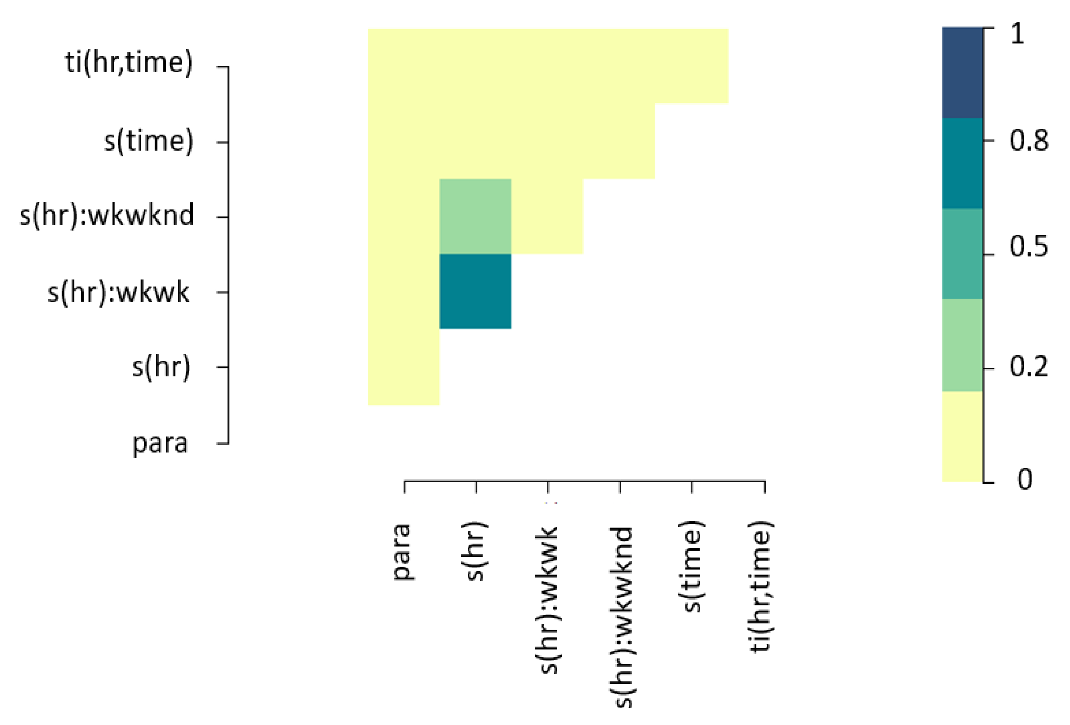
As is the case for GAMs, the correlation among covariates was tested through concurvity instead of collinearity due to the non-linear nature of the model. As expected, there is acceptable concurvity between individual effects and interactions (See Figure 6). There is no reason to believe that smooth terms of the model approximate to other terms.

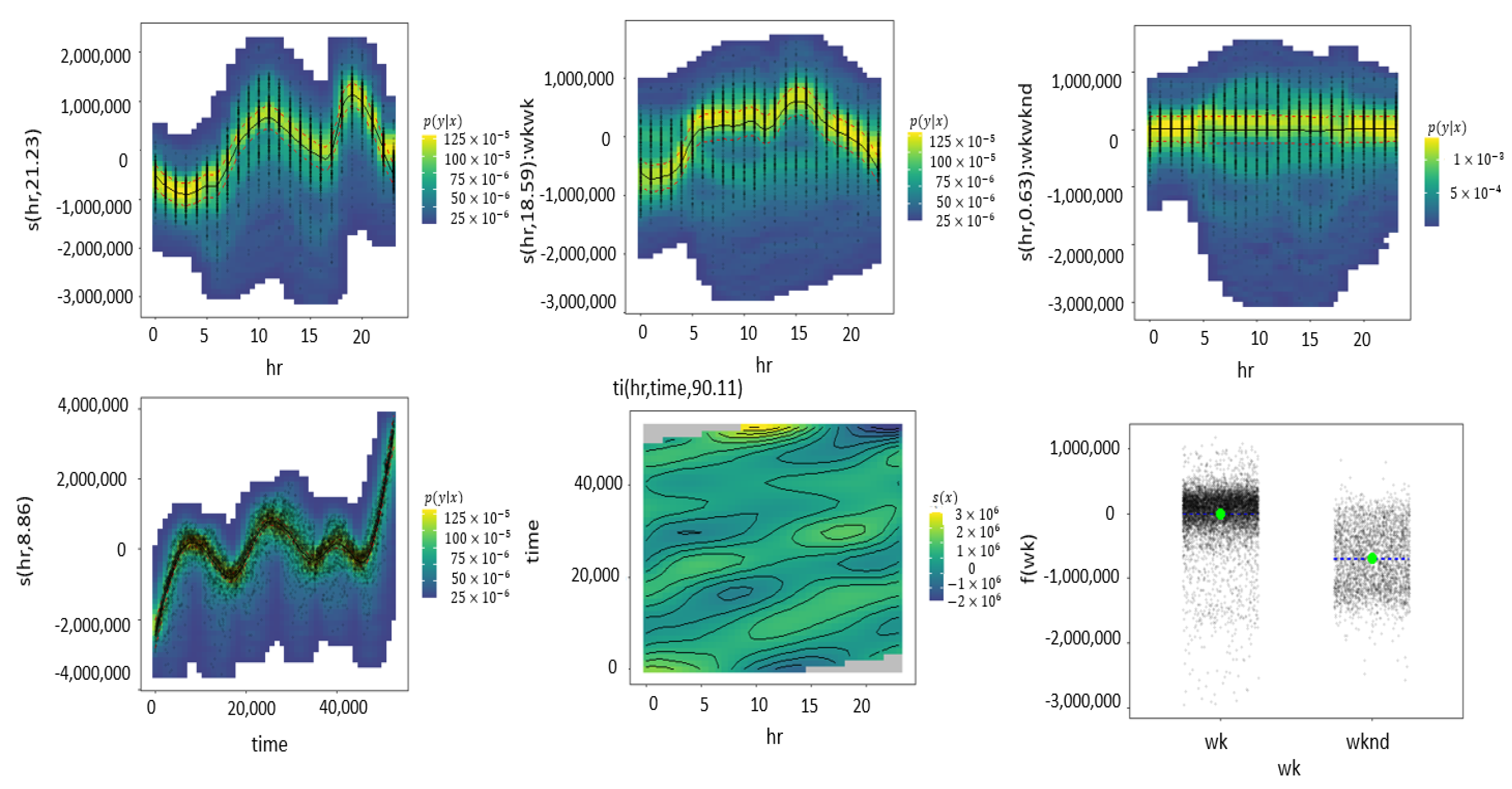
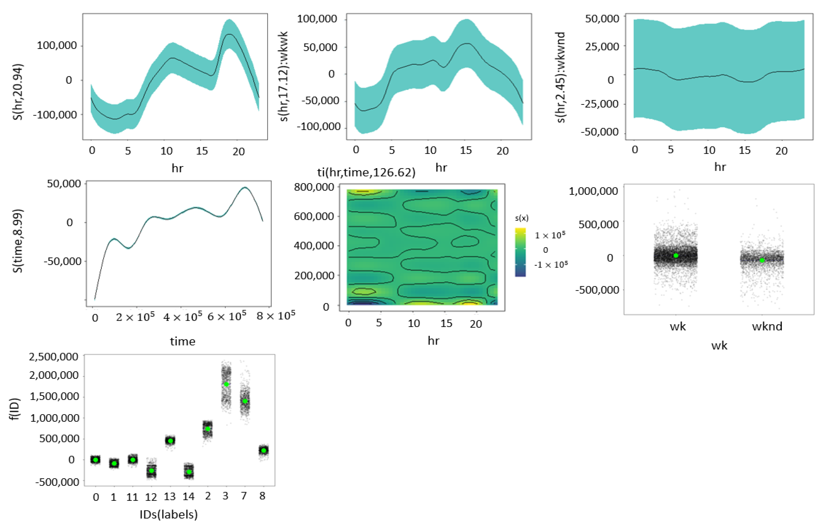
Figure 7 exhibits flat line in the density graph (first line, third figure) for the interaction of hours and weekend indicating there is no much of an effect in the interaction of such variables.On the contrary, the interaction between hours and weekdays shows a clear spline pattern in the density graph (first line, second figure). Both the individual effects of hours and data points portrayed in the first figures of the first line and second line show splines with a higher degree of curvature than the interactions.

3.2. Spatial GAM: Generalized Additive Model Regression Using Markov Random Fields as a Two-Dimensional Smoother for Modelling Space

Often, space modelling is associated with Geographically Weighted Regression, GWR [23], which according to Ref. [24] is based on the Varying Coefficient Model, VCM proposed by Ref. [25]. Although there are many other types of modelling such as the Geoadditive model [26], this one is specifically based on GLMs. In this article, the space modelling is going to be based on GAMs, as proposed by Refs. [24,27] and later incorporated by Ref. [8].

The spatial modelling will be performed through GAM using GMRF over areal data, which is often considered a separate spatial modelling technique [28] but in this case it was incorporated to the Generalized Additive Model as a two dimensional smoother so it can account for the model covariance as a function of the location, as proposed by Refs. [8,27].

Areal data is important for its various applications not only in the energy demand fields where observations could be allocated to a region according to the electricity operator but also to census and survey data where observations are aggregated to administrative districts.

Spatial GAM has the same structure as a non-spatial GAM with the addition of a term that accounts for the spatial effect represented through the smooth function $fspat\left(s_i\right)$ [27] such as

$$g\left({\mu }_i\right)=A_i\theta +\sum _{j=1}^k{L}_{ij}{f}_j\left(x_j\right)+fspat\left(s_i\right)+{ϵ}_i$$

(21)

where $d_i\sim EF({\mu }_i,\varphi )$.

In Equation (21), $A_i\theta$ accounts for the linear effects of covariates x while ${\sum }_{j=1}^k{L}_{ij}{f}_j\left(x_j\right)$ accounts for the non-linear deterministic effects defined by the smoothers and $fspat\left(s_i\right)$ accounts for the spatially correlated effect that in the equation is calculated by the GMRF.

Here the dependence of all the terms from the spatial locations is suppressed for simplicity, but it is assumed when including the Gaussian stochastic process assumptions through $fspat\left(s_i\right)$, therefore no subindex s related to the locations is included.

Equation (21) can also be represented in terms of the vector of spatial effects v [27] through an incidence matrix $R_i$, which ensures that each observation is assigned the spatial effect of the corresponding s region it belongs to by assigning ones or zeros according to whether that observation i has been collected in that region s or not

$$R_i=R[i,s]=\left\{\begin{array}{c}1\hfill \\ 0\hfill \end{array}\right.$$

(22)

which translates to

$$g\left({\mu }_i\right)=A_i\theta +\sum _{j=1}^k{L}_{ij}{f}_j\left(x_j\right)+R_{i}v+{ϵ}_i$$

(23)

After establishing the Generalized Additive Model, GAM, this article will proceed to explain the assumptions under the spatially varying effects vector, v.

To understand how the spatially varying effects vector v operates and its underlying assumptions, it is necessary to briefly recapitulate the fact that the spatial effect vector forms part of a spatial function $fspat\left(s_i\right)$ expressed as $R_{i}v$ for the specific case of discrete spatial areal data. v distribution follows a Gaussian Markov Random Field, GMR,F prior distribution conditional on the variance parameter ${\tau }^2$ [24]. In numeral 2.3, it was mentioned how Gaussian Markov Random Fields, GMRFs, follow a multivariate normal distribution such as $XN(\mu ,\Sigma )$. In this case the multivariate normal model does not fully specify the join distribution of $\gamma$ because the variance $\Sigma$ is known and denoted as ${\tau }^2$, but $\mu$ is a completely unknown reason, which is why we say that the prior is an improper prior, making the Gaussian Random Field be an Intrinsic Gaussian Random Field, IGMRF [29]. The use of improper prior distributions is widely done and preferred in Bayesian statistical analysis when the information about parameters is weak or missing [30]. According to Ref. [15], Intrinsic Gaussian Random Fields, IGMRFs, can be defined in both regular or irregular lattice. A lattice is a structure or pattern for arranging an area of land into spatial units called sub-areas, cells, or units [31]. As stated in Ref. [31] these sub-areas share boundary edges between a single or more sub-areas and cannot intersect with each other. As regards the regularity or irregularity nature of the lattice, it all depends on the application over which spatial data is going to be analysed. Radar data, for example, is usually based on regular grids because the sub-areas formed have the same shape and size. However, when the spatial data are administrative regions, as in this case, then the nature of the lattice is irregular because they are defined following the natural shape of the territory, often setting boundaries according to natural features such as rivers or mountains. This applies only for first level divisions of a country such as states or departments. The ones that follow census units are not related with the territory but are more defined for data collection purposes. Due to the idea being to estimate $X-\mu$ from the spatially varying effect vector v, then the deviation between spatial parameters v of adjacent regions such as $v_s-v_r$ will proceed to be measured, which carefully corresponds to the form of a random walk of first order such as $v_s-v_{s-1}={ϵ}_s$ with ${ϵ}_s\sim N(0,{\tau }^2)$, where s exists in a set of regions $S=\{s_1,s_2,\dots ,s_n\}$ ordered in a neighbourhood structure called ${\delta }_s$ where ${\delta }_s\subset S$ [27], which is what Ref. [15] define as a First-order intrinsic GRMF on irregular lattices and for which they use the German regions as an example. So, basically, a first-order intrinsic GRMF on irregular lattices as defined in Ref. [15] and later used an incorporated as a spatial smoother for modelling Generalized Additive Models by Refs. [8,27] is an independent Gaussian relationship between neighbouring regions i and j such as $v_s-v_r\sim N(0,{\tau }^2)$, also called an independent Gaussian increment or deviance between adjacent regions, which yields to the multivariate Gaussian Intrinsic GMRF prior, as denoted by Ref. [27].

$$p\left(v\right|{\tau }^2)=\frac{1}{2{\pi }^{(n-1)/2}{\left({\tau }^2\right)}^{(n-1)/2}}exp\left\{-\frac{1}{2{\tau }^2}\sum _{s\in S}\sum _{r\in {\delta }_s,r<s}{(v_s-v_r)}^2\right\}$$

(24)

This relation or deviance between the adjacent region shown in Equation (24) as ${\sum }_{s\in S}{\sum }_{r\in {\delta }_s,r<s}{(v_s-v_r)}^2$ and [15,32] can also be represented as ${\sum }_{s\sim r}{(v_s-v_r)}^2$, where $s\sim r$ symbolizes the set of all unordered pairs of neighbours. The pairs are defined as unordered to prevent double-counting due to the fact that if s is a neighbour from r, the order in which they get expressed $s\sim r⟺r\sim s$ does not matter, as seen before in numeral 2.3.

The quadratic form ${\sum }_{s\in S}{\sum }_{r\in {\delta }_s,r<s}{(v_s-v_r)}^2$, which represents the difference between the X vector and the $/mu$ vector in the multivariate Gaussian prior of the GAM. can also be expressed in a matrix-vector form as shown in Refs. [24,27,33].

Where v is the spatially varying vector, $v^{\prime }$ is the transposed version of the spatially varying vector, and K is a precision matrix, otherwise known as Q [15].

Letting $N_s$ represent the number of neighbours for region s such as $N_s=\left|{\delta }_s\right|$ the elements of the K precision matrix from Equation (23) as

$$K=K_{sr}=\left\{\begin{array}{c}{N}_{s}s=r\hfill \\ -1s\sim r\hfill \\ 0otherwise\hfill \end{array}\right.$$

(25)

The super index of $n-1$ could be expressed as the rank of improper precision matrix K $rank\left(K\right)=rk\left(K\right)$ [34]. The precision matrix K is called improper because it does not have a full rank. The rank of the precision matrix K from an Improper GRMF of order k is usually expressed as $n-k$ [15].

Ref. [27] states that the multivariate Gaussian Intrinsic GMRF prior for spatial effects vector $\gamma$ expressed in Equation (21) and its corresponding equivalent Equation (23) can also be articulated under full conditionals as

$$v_s|v_{-s}\sim N\left(\frac{1}{N_s}\sum _{r\in {\delta }_s}{v}_r,\frac{{\tau }^2}{N_s}\right)$$

(26)

Equation (26) can also be expressed in terms of known unequal weights based on the extent of the common boundary or the distance to the region centroids [27,32]. but the application in this document is going to be restricted to equal weights $w_{sr}=1$ for each neighbouring regions $s\sim r$, making $w_{sr}$ have no effect over the Equation (26), which is why we are not including it.

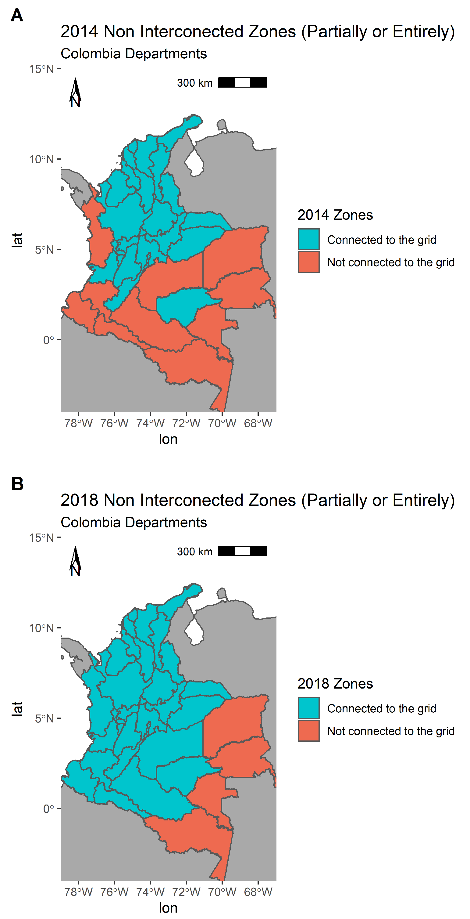
In order to run the spatial GAM, data was aggregated into regions based on the energy operators, as previously mentioned.

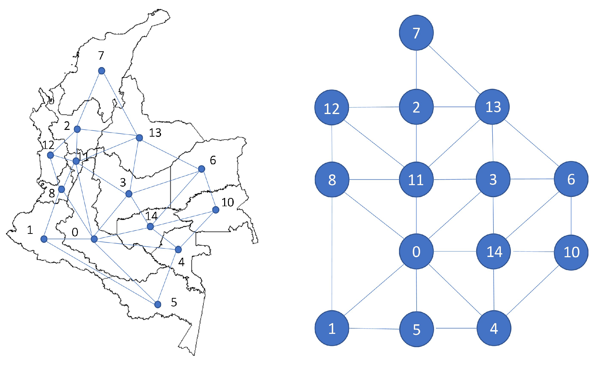
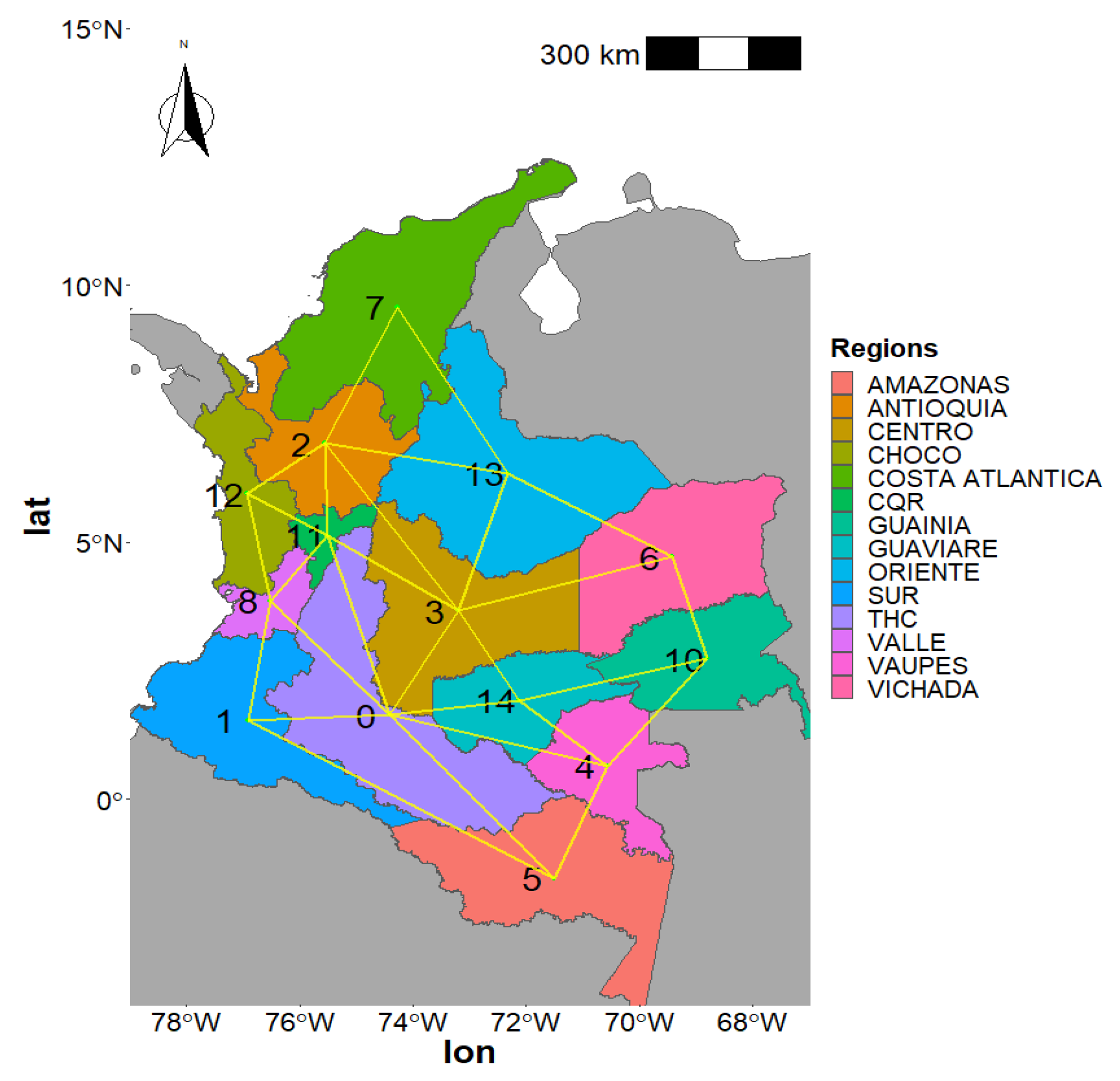
The Spatial Component from the GAM was defined using a neighbourhood structure to get a precision penalty matrix K for the regions. Neighbouring regions were defined by making a neighbours list for each region based on contiguous borders, as shown in Figure 8.

This model can be expressed as Geoadditive regression because it has no further terms but the one with the spatial component such as

$$g\left({\mu }_i\right)=R_{i}v$$

(27)

where $R_i=R[i,s]$ is the incidence matrix between observation i and region s in which the observation i was collected, and v is the spatially varying effects vector that follows a Gaussian Markov Random Field, GMRF, prior distribution conditional on the variance parameter ${\tau }^2$ such as $v_s\left|v\right(-s)\sim \frac{1}{N_s}N\left(1/N_s{\sum }_{r\in {\delta }_s}{v}_r,\frac{{\tau }^2}{N_s}\right)$ being $N_s$ the number of neighbours for region s that can also be represented as ${\delta }_s$ and in this case would represent the neighbourhood relationships shown in Figure 8.

The purely spatial GAM with Markov Random Fields has as a constraint, as it can only be limited to cross-sectional data where the precision penalty matrix K dimensions are based on the set of regions, such as K, which has $[s,s]$ dimension. This is why the application of the GMRF in this dataset was limited to aggregated data from one-year—2018.

As can be seen in

Table 5. Model summary table for spatial GAM.

Rsq	Dev	REML	Scale Est	n
0.563	0.770	48.681	42.681	14

, the resultant spatial model accounts for seventy-seve percent of the electricity demand variation. The Akaike Information Criteria AIC for this model is not truly comparable with the non-spatial GAM, which is considerably higher.

The was no need to calculate the concurvity, because the model was only dependent on one covariate, which was the Markov Random Fields, and the diagnostic showed that the model converges after five iterations, which means the data is enough for the number of parameters.

Moran’s I test was calculated to test the spatial autocorrelation in the data, and, as can be seen in

Table 6. Moran’s I test under normality spatial GAM.

Moran-I Statistic Stand Deviate	p-Value
0.99897	0.15890

and

Table 7. Moran’s I test sample estimates of spatial GAM.

Moran-I Statistic	Expectation	Variance
0.06986	−0.07692	0.02158

the value obtained showed no autocorrelation meaning the assumption of independence was maintained.

3.3. Extension of the Non-Spatial GAM with a Spatial-Categorical Regional Component

After running both temporal and spatial models as separate. A final model was built, where a covariate accounting for the regions was included over the already tested temporal one. Unfortunately, there was no way of doing this with Markov Random Fields across longitudinal data.For this reason, it was decided to use a categorical variable that had the ID of the regions such as

$$\begin{array}{c}\hfill g\left({\mu }_i\right)=A_i+f_1^s\left(hour\right)+weekday+f_3^T\left(time\right)\\ \hfill +f_{1,2}^I\left(hourbyweekday\right)+f_{1,3}^I(hour,time)+I{D}^{spatial}\end{array}$$

(28)

The components remain the same as the ones in Equation (28) for the non-spatial GAM with the addition of the categorical component that accounts for the IDs of the regions. The link function keeps being Gaussian, therefore $d_i\sim N({\mu }_i,\varphi )$ is maintained.

As can be seen in

Table 8. Model summary table extended non-spatial GAM with a spatial covariate.

Rsq	Dev	REML	Scale Est	n
0.962	0.962	$6.9594\times {10}^6$	$1.8572\times {10}^{10}$	525,560

, the resultant extended non-spatial model with the spatial categorical ID variable accounts for ninety-six percent of the electricity demand variation, which is ten percent more than the temporal model by itself.

The Wald t-test from the summary in

Table 9. Parametric coefficients extended non-spatial GAM with a spatial covariate.

Var	Estimate	Std. Error	t-Value	Pr
Intercept	312,680.9	619.1	505.028	$<2\times {10}^{-16}$
wk/wknd	−70,008.7	416.6	−168.053	$<2\times {10}^{-16}$
ID1	−88,951.4	840.8	−105.791	$<2\times {10}^{-16}$
ID2	745,127.5	882.2	844.602	$<2\times {10}^{-16}$
ID3	1,809,891.3	875.7	2066.692	$<2\times {10}^{-16}$
ID7	1,407,854.7	863.1	1631.194	$<2\times {10}^{-16}$
ID8	221,853.2	840.8	263.846	$<2\times {10}^{-16}$
ID11	2565.2	857.0	2.993	0.00276
ID12	−262,552.1	869.4	−301.993	$<2\times {10}^{-16}$
ID13	457,133.2	844.0	541.619	$<2\times {10}^{-16}$
ID14	−289,039.5	848.3	−340.734	$<2\times {10}^{-16}$

and

Table 10. Smooth terms/non-parametric coefficients extended non-spatial GAM with a spatial covariate.

Var	Estimate	Std. Error	t-Value	Pr
s(hr)	20.937	22	24.376	$<2\times {10}^{-16}$
s(hr):wk/wk	17.119	22	4.751	$<2\times {10}^{-16}$
s(hr):wk/wknd	2.450	22	0.120	$8.57\times {10}^{-15}$
s(time)	8.989	9	2723.631	$<2\times {10}^{-16}$
ti(hr,time)	126.624	198	69.221	$<2\times {10}^{-16}$

for the extended model shows that all smooth terms and parametric terms are highly significant.

The Akaike Information Criteria AIC for this model was nine times higher than the non-spatial GAM which points to the non-spatial model being a better fit even when the extended model explains more of the demand variation.

The model converges after seven iterations, showing the data being enough for the number of parameters, even where the heteroscedasticity still persists for the time individual covariate and its respective interaction as shown in

Table 11. K-check extended non-spatial GAM with a spatial covariate.

Var	k	edf	k-Index	p-Value
s(hr)	22	21.2287	0.9827	0.1175
s(hr):wk/wk	22	18.5861	0.9827	0.1075
s(hr):wk/wknd	22	0.6318	0.9827	0.1050
s(time)	9	8.8768	0.8344	0.0000
ti(hr,time)	198	90.1124	0.8369	0.0000

.

Regarding concurvity, the conclusions from the non-spatial model are maintained. There concurvity of minor magnitude between the individual effects and the interactions.

For the extended model the conclusions remain the same as for the non-spatial GAM (See Figure 9). In this model there is additional information about regions not included in the non-spatial GAM. The model shows predominance in the energy consumption of regions three-Centro, seven-CostaAtlantica, and two-Antioquia when compared against other regions.

For the purpose of comparing both models, the non-spatial GAM without the ID variable was fitted again over the same dataset as the one used for the extended version, so we could run an added variable test to check if the extra variable was contributing to explain the response or not.

The results in

Table 12. Analysis of deviance table.

Resid. Df	Resid. Dev	Df	Deviance	F	Pr (>F)
525,450	$2.3855\times {10}^{17}$
525,342	$9.7571\times {10}^{15}$	108.3	$2.2879\times {10}^{17}$	113,757	$<2.2\times {10}^{-16}$

show that there is strong evidence that the spatial categorical variable does contribute to explaining the response even when an AIC test between the two models prefers the model with fewer terms.

All analyses were performed using R Statistical Software (v4.0.3; R Core Team 2020) [35]. Generalized Additive models were fitted using the mgcv R package (v1.8-33; Wood 2020) [20]. Splines were outlined using the mgcViz R package (v0.1.6; Fasiolo 2020) [36]. Pairwise concurvity was portraited with a heatmap using base R. Maps were elaborated with the ggplot R package(v3.3.2;Wickham 2020) using geometries from the special features sf R package (v0.9.6; Pebesma 2020).

4. Discussion

A holistic approach between spatial/temporal data is hard to accomplish when modelling data with Generalized Additive Models over areas instead of points (discrete-data versus continuous-data). The fact that data is limited to areas in these case regions makes it difficult to incorporate in longitudinal datasets due to methodologies that model area data across space, such as the two-dimensional smoother Markov Random Fields, are mainly designed for cross-sectional data rather than longitudinal.

Thin-Plate Spline modelling was considered as another two-dimensional smoothing methodology but was left out of scope due to data needed to be converted from areas into points using centroids. In the cases of Colombian regions, such centroids would be more than 100 km away from each other, which would lead to Thin-Plate splines not behaving as a surface but as disaggregated ellipsoids.

Due to the previously mentioned limitations of working with areal data, it was decided to first model the individual region’s IDs against the demand and verify the assumptions of spatial autocorrelation with Markov Random Fields. Then the spatial component was incorporated into a temporal extended model using a categorical parameter based on the IDs of the regions.

Areal data has limitations when visualizing the variation of the dependent variable as a function of the distance using methods such as variograms. Variograms do not work well for areal data, especially when the number of regions is not significant due to there are not enough points to conclude over the pattern and the fact of whether the data is spatially autocorrelated or not. Nonetheless, Moran’s I test seems to work equally well for checking the independence, spatial autocorrelation assumptions, regardless of the nature of the data, areal or point-based.

Areal data from wider geographical units such as regions, states, or departments do not allow for the inclusion of a space component as a non-parametric two-dimensional smoother but smaller geographical units like census units, cities, or households could potentially allow so. While household energy information has identification constraints around it. Aggregation by smaller census areas does not. Energy modelling using household information could lead to more accurate spatial modelling when used in association with population characteristics helping to drive scientific policy advice for the energy sector.

Heteroscedasticity was found to mainly be connected to the number of knots of the time variable, as shown by the k-test. Increasing the number of knots to get rid of heteroscedasticity was considered but let out of scope to avoid overfitting.

5. Conclusions

In this article, the use of Generalized Additive Models with one-dimensional and two-dimensional smoothers is proposed as an alternative to understand how the energy demand behaves across space and time. A model using isolated temporal covariates could not be as insightful as one where both time and space aspects are incorporated and would also not be making the most of the GAM features of including multi-dimensional smoothers. The practical applicability of Markov Random Fields is limited to cross-sectional data when no temporal covariates are included.In this case, regional IDs in MRFs explain up to seventy-seven percent of the response variation.

The holistic consideration of both space and time leads to the best prediction accuracy, ninety-six percent versus eighty-five percent, from the purely temporal model, but in this case it is limited to include the regional component as a categorical parameter. In order to be able to work out the inclusion of a space component as a nonparametric two-dimensional smoother rather than a parametric one, the underlying data would have to come as coordinates and preferably disaggregated to smaller geographical units. However, this level of detail, which may be common in developed countries, it is hard to acquire in developing ones.

Future work as stated in the discussion session would encompass the gathering of point-based information about around energy consumption in the country to validate conclusions obtained with areal data. Minor scale exercises with point-based data in a city or small geographical area will be sufficient to show how a national exercise could be carried and the benefits of point-based data over areal data.

Availability of point-based data would further enhance the reliability of energy modelling as policy advice.