Article

Energy Intensity, Energy Efficiency and Economic Growth among OECD Nations from 2000 to 2019

1
The Center for Economic Research, Shandong School of Development, Shandong University, Jinan 250100, China
2
School of Environment and Society, Tokyo Institute of Technology, 3-3-6 Shibaura, Minato-ku, Tokyo 108-0023, Japan
*
Author to whom correspondence should be addressed.
Energies 2023, 16(4), 1927; https://doi.org/10.3390/en16041927
Submission received: 31 December 2022 / Revised: 5 February 2023 / Accepted: 7 February 2023 / Published: 15 February 2023
(This article belongs to the Section C: Energy Economics and Policy)

Abstract

:
This study examines the energy intensity (EI), energy efficiency (EE), and economic growth, measured by the type of returns to scale (RTS), of 37 nations in the Organization for Economic Co-operation and Development (OECD) from 2000 to 2019. We apply a non-parametric approach to estimate the three measures from their consumption of four primary energy sources, such as coal, gas, oil, and zero emission (e.g., renewable and nuclear power) as inputs and gross domestic product (GDP) as an output. In this study, we have the two types of efficiency measures over time: window-based and cross-sectional-based measures. Three findings are identified from our empirical study. First, the operationally efficient group, including France, Iceland, Japan, Switzerland, UK, and USA, presented a stable status of full efficiency in the window-based efficiency measure. Iceland and Switzerland were also in the higher efficiency group based on the cross-sectional measure. Their efficiencies were high and stable over the observed periods. Second, zero-carbon-emission (e.g., renewable and nuclear) energies outperformed other energy sources (coal, gas, and oil) in terms of a potentiality of EI/EE improvement. In other words, OECD nations can improve on their EI/EE measures by reducing fuel consumption of coal, gas, and oil while maintaining their high GDP levels. Finally, four industrial nations (France, Japan, UK, and USA) had a status of unity in their EI/EE measures for zero-carbon-emission energies with decreasing RTS. These nations would increase zero-carbon emission for energy consumption to increase GDP while keeping optimal EI/EE because such changes in consumption would not largely affect EI/EE due to their constant RTS status. Iceland showed increasing RTS. The nation may improve the EI level by increasing zero-carbon-emission energy consumption and economic size. The four nations can increase zero-emission energy consumption to achieve further economic growth without observing a large deterioration of EI/EE because it is very close to constant RTS. The examination of RTS provides policy directions for the improvement of EI and EE. Switzerland showed decreasing RTS and may deteriorate the EI/EE by increasing energy consumption and the size of each economy. The remaining countries, whose degree of EI/EE measures was less than unity, showed increasing or decreasing RTS. The examination of RTS provides important implications for energy policy to enhance the degree of EI/ EE.

1. Introduction

Reducing the energy intensity (EI) of the economies is vital to achieving a carbon-neutral society with net-zero emissions (NZE) of carbon dioxide (CO2). A recent International Energy Agency report [1], titled “Net zero by 2050: A roadmap for the global energy sector”, details the global pathway to net-zero emission (NZE) by 2050 and requires all governments to significantly strengthen and successfully implement their energy and climate policies. The report says, “minimizing energy demand growth through improvements in energy efficiency makes a critical contribution in the NZE, and indicate key global milestones for energy efficiency for the NZE”. The report sets the annual EI improvements (megajoule (MJ) per USD GDP) at −4.2% over 2020–2030 and −2.7% over 2030–2050 to achieve NZE [1].
The importance of EI in combating global warming and climate change is evident from the fact that approximately 73% of global greenhouse gas (GHG) emissions originate from our energy use in the electricity, heat, and transportation sectors (Our World in Data: https://ourworldindata.org/emissions-by-sector). The modern society accepts that economic growth is closely linked to energy use, and for most advanced economies, a decoupling between energy use with GHG emissions and economic growth is increasingly important (International Energy Agency: https://www.iea.org/news/decoupling-of-global-emissions-and-economic-growth-confirmed), not only through technological advancement to improve energy efficiency but also using policy instruments to promote energy saving. Furthermore, to attain the immediate goal of CO2 emission reduction, it is critical to shift the energy sources from fossil fuel to zero-carbon-emission ones, such as renewable and nuclear power.
To partly respond to the global challenge, this study first considers that EI is part of energy efficiency (EE). Later, we prepare a figure, which visually describes the relationship between EI and EE. Then, we will analyze the relationship between energy use and economic enhancement in 37 OECD nations. In this research effort, more specifically, we first measure the degree of EI by the quantity of energy consumption and the amount of output from economic activities, that is, the gross domestic product (GDP). As a measure of energy use, EI is calculated from the amount of energy consumption required to produce a unit of GDP. A high EI level implies high energy consumption to produce a unit of GDP, thereby denoting an energy-inefficient economy. Such measure is also influenced by a nation’s industrial structure, economic size, and industrial development. This fact implies that we need to evaluate energy efficiency by comparing similar peer economies. Furthermore, it is important to investigate the EI value from a perspective of fuel mix and a ratio of actual and optimal values of EI. This aspect leads to the necessary investigation of EE measurement between EI and GDP.
It is important to mention that EI is a special case of EE, whereby both measures use GDP as a single output. The EI compares the magnitude of multiple inputs (i.e., energy consumption), given the same amount of GDP. Meanwhile, the amount of GDP is not fixed in the EE measurement. Thus, the EI measure is a special case of the EE measure.
In addition to measuring the degree of EI and EE, this research examines the level of returns to scale (RTS) as a scale measure to understand the relationship among EI, EE, and the size change of GDP in each country. The RTS measurement provides us with information on “how the unit change in EI influences the size of GDP”. Therefore, this study also needs to examine the relationship between the size of GDP and the degree of EI and EE, thus expanding the research horizon, in contrast to previous studies on EI.
Here, note that a general implication of GDP is discussed by GDP = consumption (C) + government expenditures (G) + investments (I) + exports– imports. The main contributor to GDP is consumption (C), which is usually more than half of the countries. Some countries have a larger contribution from exports than consumption, e.g., The Netherlands, Slovakia, Slovenia, Lithuania.
To attain the research purpose, this study methodologically proposes a new type of non-parametric measure, or data envelopment analysis (DEA), to assess the holistic relationship among EI, EE, and GDP. In this study, we use a data set on energy consumption and GDP related to the countries of OECD. Specifically, the GDP in this DEA study serves as an output measure, while the inputs include the level of consumption of coal, gas, oil, and zero-carbon-emission energy sources, which comprise renewable and nuclear power.
A unique feature of the proposed method (i.e., DEA) is that it is a non-parametric approach, which can avoid the specification of a function form (e.g., linear regression) among energy consumption and GDP. We conduct the holistic analysis in a time horizon to examine the type and quantity of EI reduction and economic enhancement by applying DEA-based EE. See Sueyoshi et al. [2], Glover and Sueyoshi [3], and Sueyoshi and Goto [4] for the methodological benefit and history of DEA. The proposed approach is necessary for this study because no previous research work has discussed the analytical linkage between EI and GDP in DEA-based EE and RTS.
The remainder of this paper is organized as follows: Section 2 reviews previous contributions on EI. Section 3 describes our methodological concepts of efficiency improvement, which originate from a reduction in energy consumption and economic enhancement. Section 4 discusses how DEA handles the proposed assessment in a time horizon. Section 5 describes RTS measures from the EI perspective. Section 6 summarizes and concludes the research while providing future extensions.

2. Literature Review

2.1. EI and EE in OECD Nations

Among the previous research efforts in OECD countries, we select the following six studies on EI and EE. (a) First, Azhgaliyeva, Liu, and Liddle [5] studied the determinants of EI using empirical methods and cross-country data from 44 countries over the period 1990–2016. They found that both GDP per capita and economy-wide energy prices were negatively associated with EI. They provided evidence that several policy instruments were effective in reducing EI. (b) Second, Chakraborty and Mazzanti [6] attempted to determine a long-term relationship between green energy innovation and EI by considering 21 OECD countries over 1975–2014 and using various estimators to address key econometric issues. They found long- and short-term relationships between EI and green energy innovation. (c) Third, Filippini and Hunt [7] tried to isolate core energy efficiency for a panel of 29 OECD countries by combining the approaches used in energy demand modeling and frontier analysis. Their specifications on energy demand controlled for income, price, climate, country-specific effects, area, industrial structure, and an underlying energy demand trend in order to obtain a measure of efficiency. (d) Fourth, Voigt, De Cian, Schymura, and Verdolini [8] analyzed EI trends and drivers in 40 major economies using a logarithmic mean by applying the Divisia index to a unique data set of input–output table time series, accompanied by environmental satellite data. They decomposed efficiency changes to either changes in technology or changes in the structure of the economy, studied trends in global EI between 1995 and 2007, and highlighted sectoral and regional differences. (e) Fifth, Wurloda and Noailly [9] analyzed the impact of green innovation on EI in a set of 14 industrial sectors in 17 OECD countries over the 1975–2005 period. They created a stock of green patents for each industrial sector and estimated a translog cost function to measure the impact of green innovation on EI. They found that green innovation has contributed to the decline in EI in many sectors. (f) Sixth, Fidanoski, Simeonovski, and Cvetkoska [10] used DEA and calculated the efficiency scores on minimizing energy use and losses as well as environmental emissions for a sample of 30 OECD member states during the period from 2001 to 2018. They showed that taking care of the environment does not affect efficiency in general, while the reliance on energy produced from renewable sources does slightly reduce it. Table 1 summarizes recent studies on the EI and economic growth.

2.2. Convergence of EI and EE

Three studies have focused on the convergence of EI. (a) First, Mulder and de Groot [25] evaluated EI developments across 18 OECD countries and 50 sectors over the period 1970–2005. They found that across countries, EI levels tend to decrease mostly in the manufacturing sectors, while the service sector showed more diverse trends across sub-sectors. They also conducted convergence analysis and revealed that only after 1995, cross-country variation in aggregate EI levels clearly tended to decrease, driven by a strong and robust trend break in manufacturing and enhanced convergence in services sectors. (b) Second, Liddle [26] examined world convergence of EI using two large data sets: a 111-country sample spanning 1971–2006 and a 134-country sample spanning 1990–2006. The results from both data sets revealed continued convergence. Their investigation of geographical differences revealed that the OECD and Eurasian countries have shown considerable, continued convergence, while the Sub-Saharan African countries have converged among themselves but at a slower rate than the OECD and Eurasian countries. (c) Finally, Meng, Payne, and Lee [27] examined the convergence of per capita energy use among 25 OECD countries over 1960–2010, using unit root tests in which two endogenously determined structural breaks were employed. The results indicated significant support for per capita energy use convergence among OECD countries.

2.3. DEA Applied Energy

Several studies applied a network DEA and a dynamic DEA to analyze OECD countries’ energy efficiency. These DEA models assumed a network structure or a dynamic resource allocation system in production processes. These included works by Ouyang and Yang [28] and Guo, Lu, Lee, and Chiu [29] investigating OECD countries. In addition, Keskin [30] used a slack-based network DEA approach to measure the social prosperity efficiency of OPEC member countries. Moreover, there are studies that have analyzed OECD countries from the perspectives of EI and EE and sustainable economic and financial development (Ziolo, Jednak, Savić, and Kragulj [31]) and environmental sustainability of road transport (Mo and Wang [32]). Table 2 summarizes recent research efforts, which apply DEA for energy studies.

2.4. Position of This Study

The above literature review reveals that previous studies have not explored the relationship between EE (including EI) and GDP from a perspective of relative performance measurement based on DEA efficiency and fuel mix issues. We know that several research efforts have examined EI, EE, and the economy/economic growth in relation to health care, finance, renewable energy, and innovation. Other research works have conducted research on EI and temporal convergence among countries/regions. DEA is often applied to EI and EE studies. There are some other related research topics, e.g., EE measurement and green finance and innovation. They usually utilize econometric models and simple index measures, paying attention to input-specific EI improvement, based on actual values of data.
In contrast, this study is interested in conducting a holistic assessment of how energy is consumed to produce higher GDP by applying DEA and considering an efficient fuel mix from the perspective of EI. That is, we measure EI and the economies of scale from the perspective of efficient energy allocation. There are no previous studies that have explored the research interest. We compute the linkage for 37 industrial countries belonging to the OECD from 2002 to 2019. DEA is a holistic measure of efficiency, which uses multiple components without assuming a functional form between inputs and outputs [33].
This study has two unique features to be noted. One of the two features is that we measure a potential improvement in EI, EE, and RTS through comparison between actual and optimal values (on efficiency) by fully utilizing DEA computational capability. The proposed DEA approach considers a possibility that all nations may become either efficient or inefficient. The method measures the level of inefficiency and then identifies an efficiency frontier. Based upon the frontier, we examine the level of EI and EE and the type of RTS on an efficiency frontier on which all countries exist without inefficiency. The other feature is that we compute the three measures without assuming that all countries are efficient. The efficiency assumption is widely found in economics on which conventional productivity measures in economics have depended. In contrast, this study does not make such an assumption, so that we need to measure the level of efficiency/inefficiency status.
Table 2. References on DEA applied to energy studies (2020–2022).
Author(s)YearSummaryDataMethodsMain Topic
Keskin2021 [30]Discussed social prosperity concept for the OPEC
countries and evaluated whether OPEC member countries effectively use the wealth provided by oil to
improve social prosperity.
OPEC member countries for the year of 2019Network DEA slack based measure approachDEA application to energy
Ziolo, Jednak, Savić ad Kragulj2020 [31]Tried to show the link between energy efficiency and sustainable economic and financial development. Showed a slight upward trend of total factor energy efficiency.OECD countries for the period 2000–2018 DEA and regression analysisDEA application to energy
Li, Chien, Hsu, Zhang, Nawaz, Iqbal, Mohsin2021 [34]Measured the energy efficiency, energy poverty and social welfare of developed and developing countries. Explained how energy poverty is linked with the energy efficiency.14 developed and developing countriesDEA and entropymethodDEA application to energy
Zhu, Lin2022 [35]Examined the impact of pressure brought by economic growth target on energy efficiency improvement. Suggested that economic growth pressure has hindered the improvement of energy efficiency.188 Chinese citiesDEA, regression analysisDEA application to energy
Zhao, Mahendru, Ma, Rao, Shang2022 [36]Indicated a U-shaped non-linear effect of energy efficiency-related environmental regulation on
green economic growth as well as a spatial spillover effect and spatial feedback effect.
Panel data of 286 prefecture-level
cities in China from 2003 to 2018
Metafrontier-Global-SBM super-efficient DEA model, spatial econometric modelDEA application to energy
Zhang, Patwary, Sun, Raza, Taghizadeh-Hesary, Iram2021 [37]Measured energy and environmental efficiency. Measured cross-sectional efficiency using two inputs
(energy consumption, labor force), a desirable output (gross domestic product), and an undesirable output (CO2 emission). Found that the UK ranks the highest position in terms of energy and environmental efficiency.
Some selected countries in central and western Europe from 2010 to 2014DEADEA application to energy
Yu, He2020 [38]Provided a comprehensive overview of all publications about the researches on energy efficiency based on data envelopment analysis (DEA) retrieved from the Web of Science database.A total of 1206 documents in this field, published until 2018BibliometricsDEA application to energy

3. Underlying Concepts

To increase readability, this section starts by specifying the nomenclatures used in Section 3 and Section 4, which are summarized as follows: d : slack variables of production factors; G : a column vector of outputs ( g ); i : a subscript related to the type of inputs ( x ); j : a subscript of the j th DMU (i.e., country); k : a subscript indicating a specific DMU; m : the number of inputs; n: the number of DMUs; r : a subscript related to the type of outputs; R : data range adjustments on G and X ; s : the number of output types; t : a subscript indicating a specific period; T : the number of periods; U : a column vector of dual variables related to outputs; V : a column vector of dual variables related to inputs; X : a column vector of inputs; λ : an unknown column vector of intensity (or structural) variables; ε s : a very small prescribed number, which is set at 0.0001 in this study; σ : an intercept of the supporting hyperplane; and ξ : an inefficiency score.

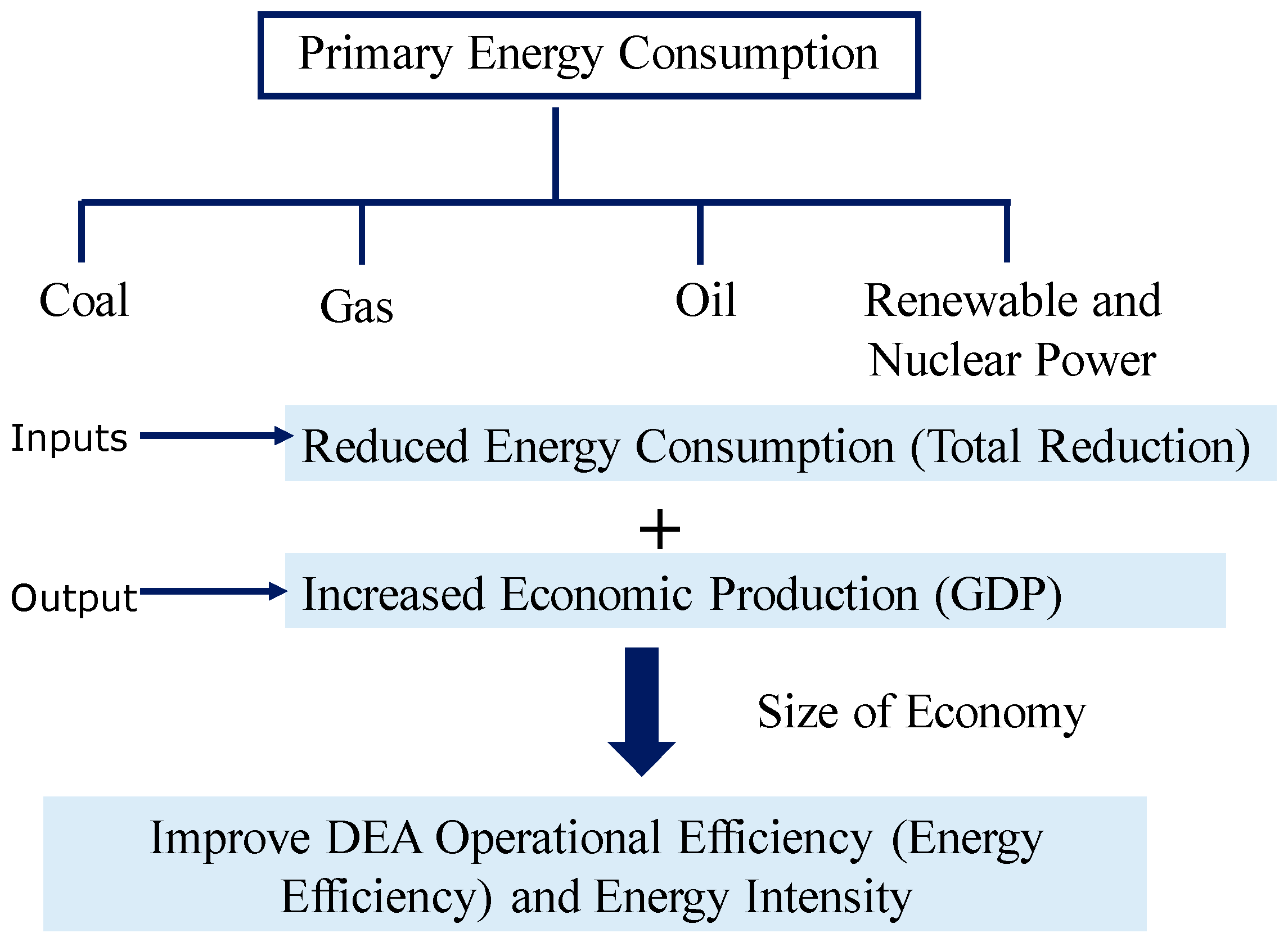
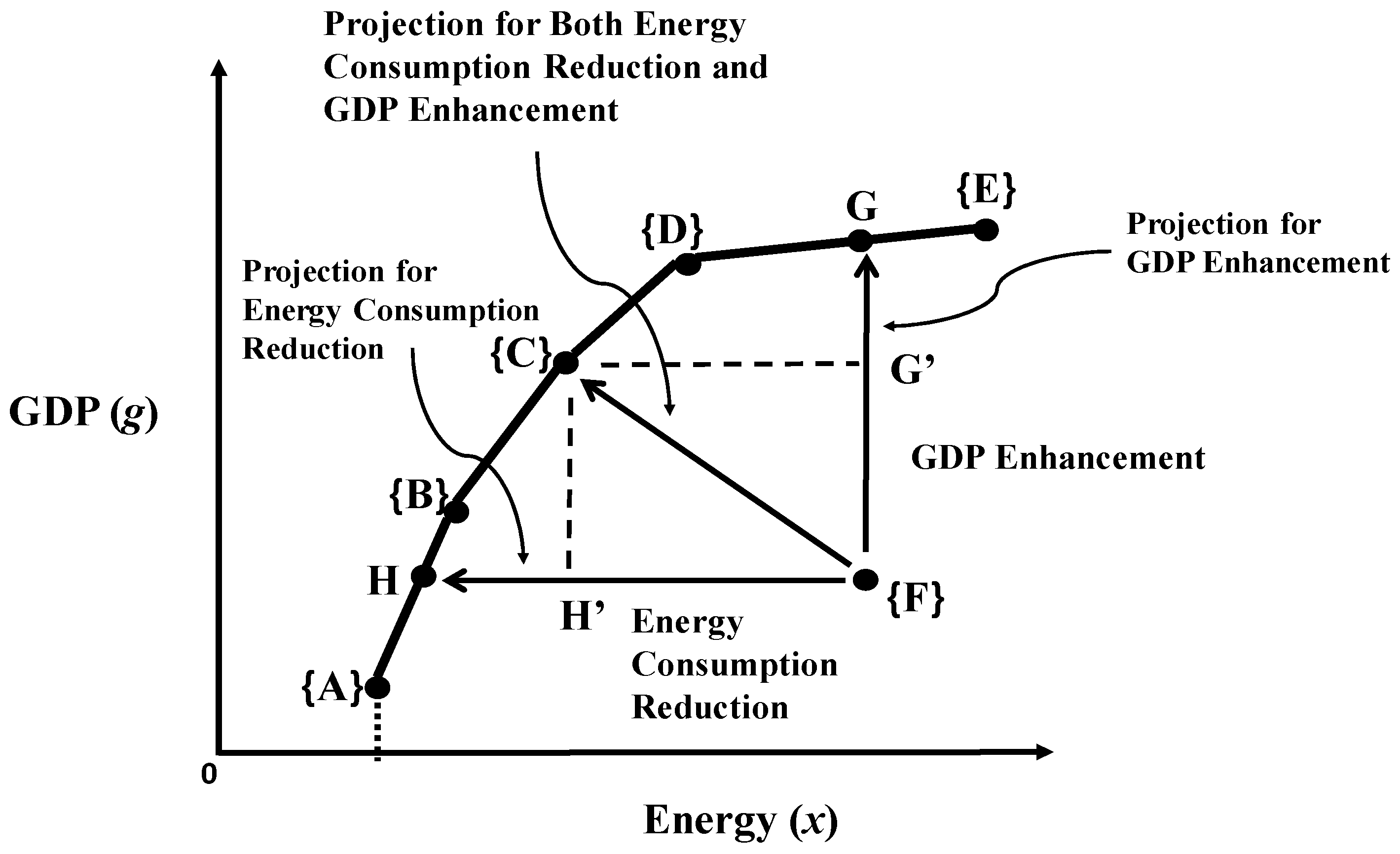
3.1. Energy Consumption Reduction and Economic Efficiency Enhancement

Figure 1 visually describes the relationship between EI reduction and GDP enhancement. In this study, energy is separated into four types of consumption: coal, gas, oil, and zero-emission (renewable and nuclear) power. Usually, a decrease in energy consumption is expected to lead to a decrease in GDP if there is no change in technology development and fuel mix. Meanwhile, we expect that this energy consumption may lead to GDP enhancement through technology development and energy mix strategy.
The figure considers that renewable and nuclear power generations have important roles in achieving a carbon-neutral society because both of them are zero-emission energy sources. Therefore, they are different from the others. Moreover, there is a noticeable movement to re-evaluate nuclear power generation. For example, the French President Emmanuel Macron announced in November 2021 that nuclear power plant construction would resume. Another example is the European Commission proposal in February 2022 for a taxonomy for climate change mitigation and climate change adaptation. Both have included the utilization of nuclear power generation as a sustainable investment. Such a change in policy direction is evident; however, in reality, it is not easy to reduce total energy consumption because human and economic activities employ energy uses. It is also not easy to replace fossil fuel with zero-emission energy because of higher cost, intermittency, and technological and social risk. Indeed, there is no perfect way to reduce EI and increase GDP simultaneously. Therefore, considering such feature of the zero-emission energy source (renewable and nuclear power), this study incorporates it as an input for efficiency measurement, as depicted in Figure 1.
Methodological importance. Figure 1 presents a methodological development, where we need to discuss the linkage between energy consumption reduction and GDP enhancement in a framework of DEA operational efficiency, or energy efficiency, in this context. It has long been considered that DEA can provide such a holistic measure. However, note that the straightforward use of standard DEA does not have such methodological capability. For example, it can measure the level of efficiency ( θ ) of the specific k th DMU. The superscript symbol (*) denotes the optimal solution of the variable obtained from the DEA model. The level of efficiency is referred to as “OE ( θ : operational efficiency)”, along with its related slacks ( d i x and d r g ) in this study. Conventionally, it has been conventionally referred to as “technical efficiency”. See Sueyoshi and Goto [4] for a historical rationale on the use of OE. Later, OE becomes EE in this study. The DEA community uses OE, but it indicates EE in energy studies. Since EE is the case of a single output in the OE measurement, we fully utilize DEA to measure the level of OE.
The level of the input-based OE ( θ ) is measured for optimality in the following manner [4]:
O E ( i n p u t ) = θ ε n i = 1 m d i x + d r g .
This type of efficiency measure originates from reducing the level of energy consumption, such as oil and gas, which serve as inputs in this study. The reduction is an input-based measure to improve the level of OE measures.
Meanwhile, the output-oriented OE is measured by an inefficiency measure ( τ ) as follows [4]:
O E ( o u t p u t ) = 1 / τ + ε n i = 1 m d i x + d r g .
This type of efficiency measure originates from economic (GDP) enhancement. The GDP serves as a single output in this study. The increase leads to OE enhancement.
Conventional difficulty. Both Equations (1) and (2) are derived from the standard DEA models. One difficulty of the two standard models is that “they have different efficiency measures [i.e., O E ( i n p u t ) O E ( o u t p u t ) ]”. As a result, we encounter a difficulty in evaluating the performance of OECD nations. Different input/output models produce different OE measures. Therefore, we wonder what is our final answer on OE? In contrast to the difficulty of previous DEA measures, this study unifies the input-oriented (energy consumption) and output-oriented (GDP) measures to identify a single measure as a new alternative to the standard OE measures. This is the first methodological contribution.
Visual Description. Figure 2 consists of an input ( x : energy consumption) on a horizontal axis and an output ( g : GDP) on a vertical axis. The figure depicts the input-oriented projection, implying energy consumption reduction, and the output-oriented projection, implying GDP enhancement, both of which increase the DEA-based OE measures, or energy efficiency. In the figure, a frontier consists of efficient decision-making units, or DMUs {A-B-C-D-F}, while {F} is “inefficient” because the DMU, an OECD nation in this study, is located within the efficiency frontier. Here, let us explain the three possible projections from inefficiency to efficiency. First, the input-oriented model uses a projection, which shifts {F} to H on the frontier for efficiency enhancement. This type of projection is measured in Equation (1) for “energy consumption reduction”, projection {F} to H. The projection implies that given a fixed amount of GDP, it indicates an amount of energy consumption reduction to attain the status of OE. Second, the output-oriented model projects from {F} to G, which focuses on “economic (GDP) enhancement”. This projection implies that given an amount of energy consumption, it enhances the amount of GDP to attain the status of full OE. This type of projection is measured by Equation (2). In the third case (in the proposed approach), if we can project {F} to {C}, then the projection attains both energy consumption reduction and GDP enhancement. As depicted in Figure 2, all the projections may change the status of inefficiency to efficiency on the frontier. The approach proposed in this study uses the third type of projection, different from Equation (1) (energy consumption reduction) and Equation (2) (economic (GDP) enhancement).

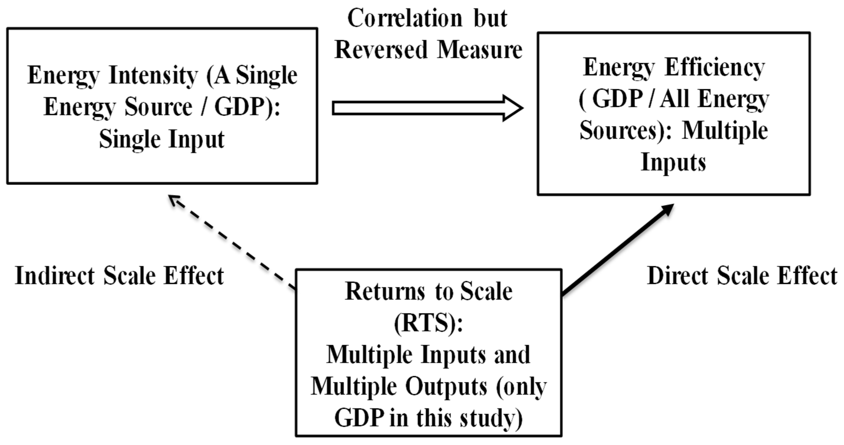
3.2. A Scale Effect on Energy Intensity and Energy Efficiency

Figure 3 visually describes a rationale on why the RTS measurement is necessary to understand both EI and EE (e.g., OE in this study). They are clearly influenced by the size of each nation. For example, the two measures of the USA are structurally different from a small OECD nation. The GDP (as a scale of the economy) of the USA is the largest in the world. It is easily imagined that there is correlation between EI and EE, even if both are different measures. The EI is measured by a single energy source consumption divided by GDP, while the EE is measured by GDP divided by all energy source consumptions. They are clearly influenced by the size of each nation and its energy and industrial structures. Therefore, as a scale measure, we need to measure the RTS of all OECD nations in terms of energy consumption. No previous study has documented the research concern.

3.3. Strengths and Shortcomings of DEA

The strengths and shortcomings of DEA are summarized as follows. First, DEA is able to incorporate multiple inputs and multiple outputs, where we do not assume any functional form that specifies the relationship between them. It is not impossible but difficult for us to handle multiple outputs by using standard economics. Second, DEA can measure the degree of OE by a percentile expression (i.e., 0 is full inefficiency and 1 is full efficiency), so that we can assess the performance of public and private entities. A drawback of DEA is that we cannot use it for forecasting, as found in statistics and econometrics. Third, DEA estimates a production function by piece-wise linear approximation, which connects the observed data on an efficiency frontier (e.g., {A}-{B}-{C}-{D}-{E} depicted in Figure 2). Finally, DEA does not assume any error distribution (e.g., a normal distribution). It is true that such DEA capability is useful and important for performance assessment. However, DEA is not capable of any statistical inferences and tests. We must use DEA along with statistical analysis. This is another shortcoming of DEA.

4. Formulations for Measurement in a Time Horizon

All formulations discussed in this research are relatively new, particularly when applied to energy research. One exception is a study by Sueyoshi et al. [2]. The study prepared by Sueyoshi and Goto [4] has documented almost all DEA research efforts applied to energy which were listed in the Science Citation Index (SCI) and the Social Science Citation Index (SSCI), from 1978 to 2017. See also Sueyoshi et al. [39] for a literature review on 693 research efforts on DEA and DEA-based environmental assessment. To the best of our knowledge, all formulations in this research are different from them, fitting the scope of this research purpose. Here, we note that the proposed approach has three methodological extensions. First, the previous assessment separates production factors into input-oriented and output-oriented measures. Both produce different estimates of efficiency in DEA measurement. The proposed approach unifies the two measures and produces a unique efficiency measure. Second, it incorporates a time horizon through which we can capture the changes in time among multiple annual periods. Finally, we measure the type of RTS to examine how the size of energy consumption and GDP influence the EE of each nation.

4.1. Cross-Sectional Operational Efficiency (CSOE)

To extend the proposed OE (= EE) measurement into a time horizon, we use two different measures. First, we pool all of their observations on DMUs in a cross-sectional structure. This type of OE measure is a straightforward extension, which includes a time horizon. Therefore, we refer to it as “CSOE”. The measure is used as the basis for a relative comparison; for example, it investigates the statistical difference among different periods and groups by using a rank-sum test. This is the methodological benefit of CSOE.
To describe the CSOE measurement, let us consider each entity as a DMU to be evaluated. Regarding each DMU, the energy with m components ( X : energy consumption) is transformed by the production technology into an economic performance measure with a single output ( g : GDP). Any functional form is not assumed in this research to specify the relationship between X and g . DEA connects them by multipliers, or weights, among them. Thus, the approach estimates weights (so-called multipliers), not parameters; it is therefore “non-parametric” and avoids any specification error of a functional form.
Projection. This study utilizes a new type of DEA, which determines the level of OE of the specific k th DMU at the specific t th period ( t = 1, …, T ). An important feature of the proposed measurement is that it evaluates the performance of each DMU given observed X k t and g k t . The observation ( X k t and g k t ) serves as the directional vector on which each DMU changes the status from inefficiency to efficiency, as shown in the projection from {F} to {C} in Figure 2. The standard DEA models did not have such directional vector, as discussed previously.
Before discussing the formulations used for this research, we note two concerns. One of the two concerns is that we use the subscript ( j ) to specify all DMUs ( j = 1, …, n ), while the subscript ( k ) indicates a specific DMU to be evaluated. The other concern is that this study also uses the subscript ( z ) to indicate all periods ( z = 1, …, T ), while the subscript ( t ) indicates a specific period to be evaluated.
As the first formulation, this study measures the degree of cross-sectional operational efficiency ( C S O E k t v ) of the specific k th DMU at the specific t th period using the following formulation, where the superscript ( v ) indicates variable RTS. See Sueyoshi et al. [2].
Maximize ξ k t + ε s i = 1 m R i x d i t x + R g d t g s . t . z = 1 T j = 1 n x i j z λ j z + d i t x + ξ k t x i k t = x i k t   ( a l l   i ) , z = 1 T j = 1 n g j z λ j z d t g ξ k t g k t = g k t z = 1 T j = 1 n λ j z = 1 , λ j z 0   j = 1 , , n   &   z = 1 , , T ,   ξ k t : U R S , d i t x 0   a l l   i   &   d t g 0 .
An efficient frontier of DMUs for all periods ( z = 1, …, T ) is formulated by the left-hand side of Model (3). A crossover may be contained in the efficiency frontier between or among multiple periods, and thereby, the frontier of this model consists of the best performers in all T periods. On the other hand, the right-hand side indicates the performance of the specific k th DMU in a specific period ( t ) to be examined. The observation ( x i k t and g k t ) serves as a directional vector in which Model (3) maximizes the level of inefficiency for calculation. As conventional DEA models do not have the directional vector, their efficiency measures are input-oriented or output-oriented, as specified in Equations (1) and (2). Meanwhile, Model (3) incorporates the directional vector to produce an efficiency measure, which combines both Equations (1) and (2).
The distance measures ( + d i t x + ξ k t x i k t and d t g ξ k t g k t ) indicate differences between the observed performance of each DMU and the efficiency frontier in multiple ( m + 1 ) dimensional factors (e.g., inputs and outputs). The unified inefficiency ( ξ k t ) indicates the degree of a directional vector, which should be arranged toward the efficiency frontier. The slacks ( d i t x and d t g ) express the remaining parts of the difference, which we cannot specify in measuring the level of inefficiency. The small number ( ε s ), expressing the relationship between inefficiency and total slacks, indicates a number that we need to prescribe for the operation of Model (3).
Strengths. Model (3) has an important feature, in that an efficiency score does not depend upon the energy (input) or economic (output) orientation, as found in Models (1) and (2). This feature is different from standard ratio models, which depend upon the orientation. As discussed previously, input-oriented efficiency is different from output-oriented efficiency. Model (3) does not hold such difficulty because all factors (inputs and outputs) are unified in a single inefficiency measure ( ξ k t ), and there is no difference between them. Note that the standard models originated from the ratio model; therefore, they suffered from the methodological difficulty.
The degree of C S O E k t v of the k th DMU in the t th period is measured by
C S O E k t v = 1 ξ k t + ε s i = 1 m R i x d i t x + R g d t g .
Here, superscript ( v ) implies “variable” RTS in Model (3). The optimality (*) of Model (3) determines the inefficiency measure ( ξ ) and all slack variables ( d i t x and d t g ), and the degree is obtained by subtracting the level from unity, as specified in Equation (4).
Strength. The important feature of Model (3) is that it puts an inefficiency measure ( ξ ) before inputs and outputs. The optimization attempts to minimize the level of inefficiency. Such two features cannot be found in the previous DEA studies, except in Ref [2]. As a result, the projection is uniquely determined. Such are the strengths of Ref [3].
Drawbacks. Both Equations (3) and (4) incorporate an assumption that DMUs at the t th period (past) can access the future technology in the z periods. Such assumptions are a methodological shortcoming. The other difficulty of the C S O E k t v , measured by Model (3), is that all DMUs in the future are assumed to access an efficiency frontier (therefore, technology) in the past. An opposite case is also true. This is problematic. For example, the structure of Model (3) incorporates an assumption that DMUs in 2020 may utilize technology in the past, e.g., 2000, for their operations. Such assumption is often not practical to implement in most industries because they must consider business competition in the global market. This indicates a drawback of Model (3). In reality, DMUs mostly utilize technology that is as recent as possible to meet the global competition.
At the end of the C S O E k t v description, it is necessary for us to specify the following data ranges on X and g used in Model (3). Here, R i x is a data range on the i th input ( m components), and R g is a data range on the output (a single component: GDP).
R i x = ( m + 1 ) 1 m a x j t x i j z   f o r   a l l   j   &   a l l   t m i n j t x i j t   f o r   a l l   j   &   a l l   t 1 ,
R g = ( m + 1 ) 1 m a x j t g j t   f o r   a l l   j   &   a l l   t m i n j t g j t   f o r   a l l   j   &   a l l   t 1 .
The data ranges are applied to all DMUs ( j = 1, …, n ) in all periods ( t = 1, …, T ) in the proposed DEA models, so that the DEA results are able to avoid a possible occurrence of zero in dual variables (i.e., multipliers). Such a possible occurrence implies that corresponding production factors ( X and g ) are not fully utilized in DEA assessment, which is problematic in DEA applications. To avoid the difficulty, this study incorporates the data ranges (5) and (6) to fully utilize the available information on X and g .

4.2. Window-Based Operational Efficiency (WOE)

To overcome this drawback of Model (3), this study utilizes the concept of “window analysis”, which combines recent periods into a time horizon to be examined. We use the following window-based approach to measure the level of window-based operational efficiency ( W O E k t v ) on the k th DMU at the specific t th period.
Maximize ξ k t + ε s i = 1 m R i x d i t x + R g d t g s . t . z W t j = 1 n x i j z λ j z + d i t x + ξ k t x i k t = x i k t   ( a l l   i ) , z W t j = 1 n g j z λ j z d t g ξ k t g k t = g k t , z W t j = 1 n λ j z = 1 , λ j z 0   a l l   j   &   z W t ,   ξ k t : U R S , d i t x 0   a l l   i   &   d t g 0 .
Here, W t (the t th window) indicates a group of recent periods (e.g., { t 2 , t 1 , t } W t ) before the specific t th period. The left side term (i.e., z W t j = 1 n x i j z λ j z and z W t j = 1 n g j z λ j z ) of Model (7) indicates an efficiency frontier, which consists of DMUs in W t , comprising variable RTS by incorporating z W t j = 1 n λ j z = 1 as a side constraint. Note that Model (7) is a general form of Equation (3). If W t covers all periods, then Model (7) becomes Model (3). The difference between the two models is the periods to be covered. Model (7) covers partial periods, while Model (3) covers all period combinations. This type of application incorporated in Model (7) corresponds to the “moving average” in forecasting (statistics).
We measure the degree of W O E k t v of the k th DMU at the t th period by
W O E k t v = 1 ξ i t + ε s i = 1 m R i x d i t x + R g d t g ,
where the inefficiency measure ( ξ ) and all slack variables ( d i t x and d t g ) within the parenthesis are determined on the optimality (*) of Model (7). Equation (8) determines the degree of efficiency by subtracting the level from unity. A historical review can be found in Refs [3,4,39].
To extend Model (7) to the scale-related (i.e., RTS) measurement of the k th DMU, we need to consider the dual formulation of Model (7), which becomes
Minimize i = 1 m v i k t x i k t u k t g k t + σ k t s . t . i = 1 m v i k t x i j z u k t g j z + σ k t 0   ( a l l   j   &   z W t ) , i = 1 m v i k t x i j t + u k t g k t = 1 v i k t ε s R i x   i = 1 , , m , u k t ε s R g   r = 1 , , s , &   σ t : U R S .
The first group contains constraints related to W t , which includes t 2 , t 1 , and t th periods, in Model (9).
Using Model (9), we measure the degree of W O E k t v of the k th DMU at the t th period by
W O E k t v = 1 i = 1 m v i k t x i k t u k t g k t + σ k t .
Here, the optimality (*) of Model (9) determines the dual variables ( v i and u ). Both Equations (8) and (10) produce the same degree of efficiency on optimality.

5. EI and RTS

5.1. DEA-Based EI

The concept of EI (as part of EE) is originally considered, as one input/GDP with both observed values. This research measures the two values based upon those in an efficient frontier. Such treatment eliminates the existence of inefficiency in practicality. To measure EI, we first discuss how to measure the level of DEA-based optimal EI. This study uses Model (7) for our measurement. For each year, + d i t x + ξ k t x i k t and d t g ξ k t g k t indicate the differences (inefficiency) from the observed performance ( x i k t and g k t ) of the k th DMU at the t th period. On an efficiency frontier, the observations are adjusted by x ¯ i k t = 1 ξ k t x i k t d i t x and g ¯ k t = 1 + ξ k t g k t + d t g , both of which are adjusted on the optimality of Model (7). We determine the EI of the optimal values of the i th input (energy consumption) of the k th DMU at the t th period by
E I i k t = x ¯ i k t / g ¯ k t = 1 ξ k t x i k t d i t x / 1 + ξ k t g k t + d t g   for   i = 1 , m .
Meanwhile, the EI of observed data (EIO) is specified by
E I O i k t = x i k t / g k t .
We use the ratio between the two EI scores (REI) measured by Equations (11) and (12) as follows:
R E I i k t = E I i k t / E I O i k t = ( x ¯ i k t / g ¯ k t ) / ( x i k t / g k t ) .
The ratio indicates a potential to improve the status of EI, more generally EE. The degree, different from unity, indicates that a gap exists between optimal and actual measures on EI. The former (optical EI) is measured on an efficiency frontier, so that it outperforms the observed one. Thus, the degree of REI is less than or equal to unity. The status of unity indicates that the specific k th DMU is empirically the best performer in EI. Similarly, if it is less than unity, the DMU needs to improve the status of EI/EE.

5.2. Return to Scale (RTS)

There are two ways to enhance the level of EI/EE. Each nation has to decrease the amount of energy consumption (x) under the given level of GDP (g), or each nation has to increase the amount of GDP (g), given x. The previous studies in Section 2 mainly discussed the first case but did not directly address the second one. Moreover, the input vector has multiple energy consumptions in this study, while the previous studies only pay attention to a single energy consumption in the EI computation. While acknowledging the contributions of these studies, we describe a new research direction on EI, i.e., a change of x components for an increase in GDP (g) using the economic concept of RTS.
To begin with, we describe the concept of “scale elasticity”. The degree of scale elasticity (eg) is conceptually specified as
eg = marginal product/average product = (dg/dx)/(g/x).
As specified in Equation (14), scale elasticity has the opposite structure of EI; that is, the degree of EI is measured by x/g, while the eg is measured by g/x and dg/dx in a simple case.
Using elasticity, we classify the concept of RTS of each DMU by the following rule:
( a )   e g > 1     Increasing   RTS ,   ( b )   e g = 1     Constant   RTS ,   and ( c )   e g < 1     Decreasing   RTS .
Furthermore, as discussed by Sueyoshi et al. [2], the three types of RTS are intuitively expressed by the intercept as
( a )   Increasing   RTS     σ < 0 ,   ( b )   Constant   RTS     σ = 0 ,   and ( c )   Decreasing   RTS     σ > 0 .
A detailed description of Equation (16) has been provided in some studies (e.g., Sueyoshi and Goto [4,33]).
To discuss a relationship for RTS in a time horizon, we start from a simple case with time, where an input ( x t ) is used to produce an output ( g t ) in the t th period. We incorporate the subscript (t) to express each period and assume that a supporting hyperplane is expressed by v t x t u t g t + σ t = 0 or g t = v t / u t x t + σ t / u t . A mathematical requirement to identify the supporting hyperplane is that u t should be positive in the sign. The variable ( σ t ), indicating a constant term of the supporting hyperplane, is unrestricted (URS) in the sign.
Note that if u t is zero, it is difficult to determine the location of a supporting hyperplane because v t / u t and σ t / u t become “infinite”. The ratio ( d g t / d x t = v t / u t ) indicates a “marginal rate of transformation”. The variable ( u t ), related to the t th output, characterizes a supporting hyperplane in a data domain of x t and g t .
Returning to Model (9), we discuss the type of RTS measured by Model (9) because it is a general form of Model (3). In the optimal solution V k t , u k t , σ k t of Model (9), each V k t is considered as a virtual input price vector of X k t . Similarly, u k t is a virtual output price for g k t . Each component of these vectors indicates a slope of a supporting hyperplane(s) on a production possibility set. Both should be positive.
As the intercept of a supporting hyperplane(s) is directly related to RTS, we determine RTS by examining a sign of the dual variable ( σ k t ). The optimal solution of Model (9) identifies the following types of RTS on the k th DMU at the t th window:
( a )   Increasing   RTS     An   optimal   solution   V t , u t , σ t   of   Motel   ( 9 )   satisfies   σ k t < 0 ; ( b )   Constant   RTS     An   optimal   solution   V t , u t , σ t   of   Model   ( 9 )   satisfies   σ k t = 0 ;   & ( c )   Decreasing   RTS     An   optimal   solution   V t , u t , σ t   of   Model   ( 9 )   satisfies   σ k t > 0 .

6. Empirical Study

6.1. Data

The data set used in this study consists of an output and four inputs from 37 OECD countries during the annual periods over 2000–2019. The output data indicate real GDP in constant 2010 million US dollars. The data set was obtained from World Bank Open Data (https://data.worldbank.org/). All input data were obtained from Our World in Data, Energy section (https://ourworldindata.org/energy). Table 3 summarizes the descriptive statistics of the data.
Since this study is interested in the DEA-based EE, EI, and RTS of the OECD countries, the GDP here represents the total value added in a country as an output, and the four inputs are primary energy consumptions of coal, gas, oil, and zero-carbon (carbon-neutral) energy sources. All were measured in terawatt hours (TWh), as provided in the data source. The fourth input of energy consumption is derived from carbon-neutral energy sources from nuclear power and renewable energy, such as biofuel, solar power, wind power, hydro power, and other sources.

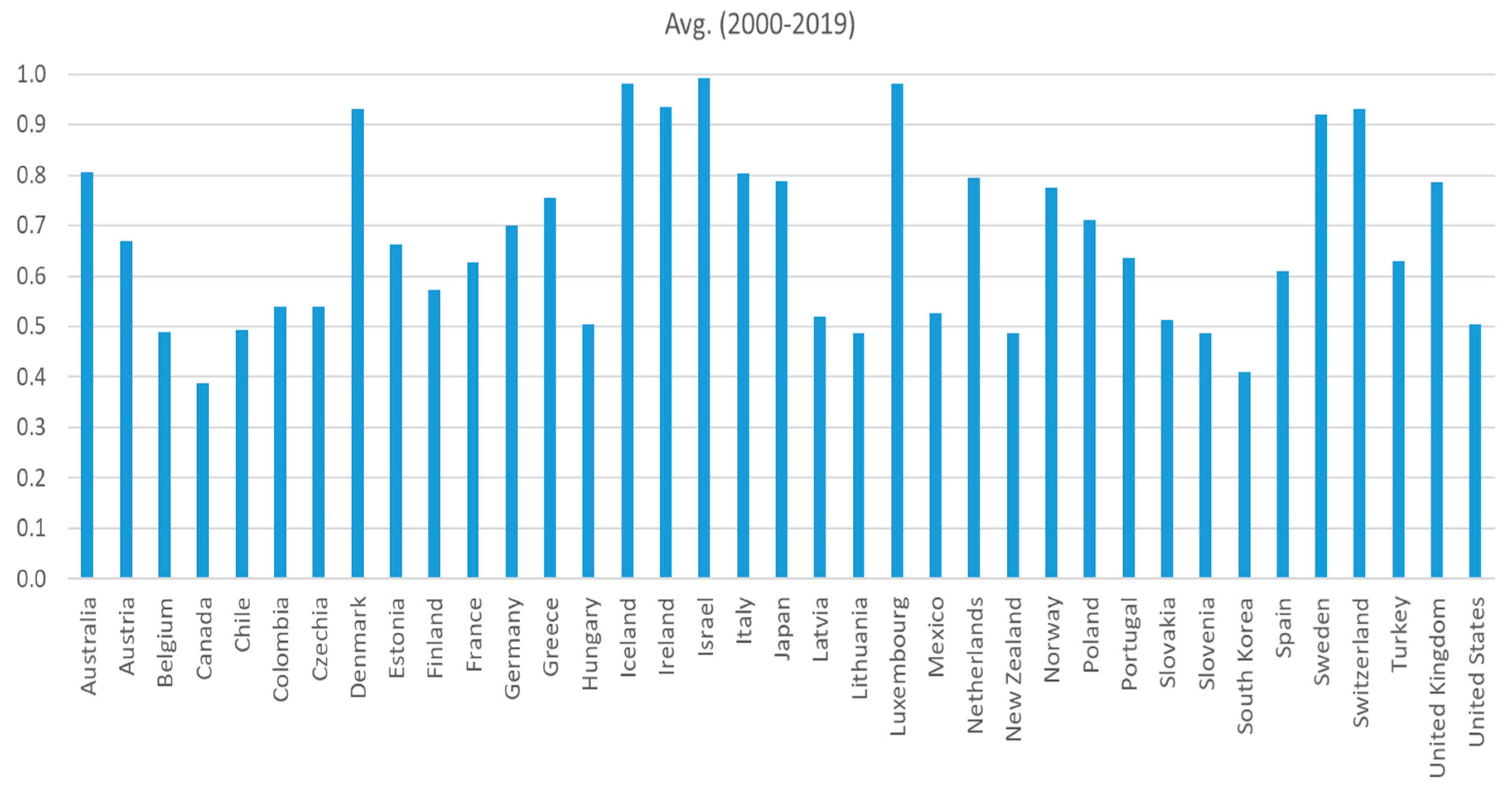
6.2. OE, EI, and RTS Measures

As an illustrative example, Table 4 summarizes the CSOE measures of the 37 OECD nations in 2000 and 2019 (both are illustrative examples) and the total average from 2000 to 2019. We computed the efficiency measures using Model (3), and the degree of these efficiencies was determined by Equation (4). Figure 4 visually describes the average of these efficiency measures of 37 nations from 2000 to 2019. Their efficiency (CSOE) scores, based upon a cross-sectional structure, were measured by Model (3), where we treated all data sets from 2000 to 2019 as a single data set. The left-hand side (under avg.) of Table 4, along with Figure 4, shows that Denmark, Iceland, Israel, Luxembourg, Sweden, and Switzerland have exhibited high (more than 0.9) annual average of CSOE. The result implies that they showed higher CSOE performance than other OECD nations.
Next, changing the OE measurement from CSOE (cross-sectional) to WOE (window), Table 5 summarizes the energy efficiency measures from the window analysis of the 37 OECD nations from 2002 to 2019. This type of efficiency measure (WOE) assumes an annual shift, which is more clearly identified than CSOE. Figure 5 visually describes the average of annual efficiency changes of 37 nations from 2002 to 2019. The efficiency scores were measured by Model (7). Table 5 clearly indicates a group of nations whose average efficiencies are unity, comprising France, Iceland, Japan, Switzerland, the UK, and the USA. These countries present a stable status of full efficiency in moving across the window periods. Both Iceland and Switzerland are included in the higher efficiency score group in CSOE and are also classified as full efficiency countries in WOE, as their efficiencies are high and stable over the periods.
Table 6 summarizes the REI measures of each energy consumption source in 37 OECD nations in 2019, for example, because the year is the latest annual period. It is interesting to note that, as listed at the bottom of Table 6, zero-carbon energy has outperformed the other energy sources (coal, gas, and oil) in terms of REI in 2019. In other words, the observed EI of zero-carbon energy is close to the optimal values, which are determined by the WOE models. Table 7 shows France, Iceland, Japan, Switzerland, the UK, and the USA attaining unity in the degree of REI for zero-carbon energy. That is, these nations have DEA-based optimal EI values.
Table 8 presents the results of RTS measures, where the optimal σ t calculated from Model (9) identifies the degree and type of RTS by following Equation (16). They indicate that most OECD countries are classified into two groups: (a) the increasing RTS group with negative intercepts and (b) the decreasing RTS group with positive intercepts. The former (increasing) includes smaller countries, such as the Czech Republic, Estonia, Finland, Hungary, Latvia, Lithuania, New Zealand, Norway, Slovakia, and Slovenia. The latter (decreasing) group includes larger economies, such as Australia, Belgium, Canada, France, Germany, Italy, Japan, Mexico, The Netherlands, Poland, South Korea, Spain, Turkey, the UK, and the USA. The results indicate that the larger economies have a decoupling status between energy consumption and GDP, where the economies are relatively independent from energy consumption, which may be brought about by their sustainable industrial structures, fuel mix, and energy-saving technologies.
Looking into the last column (average) of Table 7 and that of Table 8, this research finds three important implications. First, four industrial nations—France ( σ t = 0.0659), Japan ( σ t = 0.0285), the UK ( σ t = 0.0252), and the USA ( σ t = 0.0745)—have a status of unity in their degrees of REI for zero-carbon-emission energy and belong to decreasing RTS, but their degree of σ t is very close to constant RTS. Thus, these nations can increase zero-emission energy consumption to increase the GDP while keeping optimal EI because the influence of such changes is limited due to their near-constant RTS.
Second, among the nations with unity in REI, Iceland shows −0.5185 on average σ t ; therefore, it is increasing its RTS. The nation may increase zero-emission energy consumption to increase the GDP while attaining further improved EI due to the increasing RTS. On the other hand, Switzerland shows 0.4806 on average σ t and decreasing RTS; therefore, if it increases zero-emission energy consumption to increase the GDP, it may deteriorate EI and REI by increasing its GDP.
Finally, the remaining countries whose REI measures were less than unity had positive or negative σ t , and decreasing or increasing RTS. For example, Australia showed 0.0471 on average σ t , implying decreasing RTS. Meanwhile, the Czech Republic showed −0.0557, indicating increasing RTS; therefore, increased zero-emission energy consumption and GDP may improve their EI and enhance the degree of REI. Thus, the type of RTS is worth examining to discuss the energy policy to enhance the degree of EI under economic prosperity.

7. Conclusions and Future Extensions

This study discussed how to measure the DEA-based EE, EI, and RTS of 37 OECD nations during 2000–2019. We applied a new type of DEA approach with cross-sectional and window analyses to a data set consisting of four energy consumption sources (coal, gas, oil, and zero-carbon-emission energies) to produce the GDP. The new DEA models incorporated a directional vector to identify the degree of EE of these industrial nations. After examining their efficiency scores, we discussed the measurement of EI and REI of the OECD nations. Finally, we re-examined their EE and EI statuses based on their RTS statuses. The combined use of REI and RTS provides the policy direction on future energy consumption for GDP enhancement.
After completing the methodology development, we obtained the following three implications from the application to the 37 OECD nations. First, the efficient group of six countries—France, Iceland, Japan, Switzerland, the UK, and the USA—presented a stable status of full efficiency in WOE. Iceland and Switzerland were also in the higher efficiency group based on CSOE. Their operational efficiencies were high and stable over the observed periods. Second, zero-carbon-emission (renewable and nuclear) energies outperformed the other energy sources (coal, gas, and oil) in terms of REI, a potentiality of EI improvement. In other words, OECD nations can improve further on total EI by reducing fuel consumption of coal, gas, and oil while maintaining GDP levels. Finally, four industrial nations—France, Japan, the UK, and the USA—had a status of unity in their REI measures for zero-carbon-emission energy with decreasing RTS. These nations would increase zero-carbon-emission energy consumption to increase the GDP while keeping optimal EI because such changes in consumption would not largely affect the REI due to their constant RTS. Iceland showed increasing RTS and may improve its EI level by increasing zero-carbon-emission energy consumption and economic size. Switzerland showed decreasing RTS and may deteriorate EI by increasing energy consumption and the size of the economy. The remaining countries, whose REI measures were less than unity, showed increasing or decreasing RTS. The examination of RTS type provides interesting implications for potential improvement of EI and energy policy direction to enhance the degree of REI and economic growth.
This study proposed a holistic approach for measuring EI, EE, and RTS by applying DEA from the perspective of efficient energy allocation or an efficient fuel mix. Further, we demonstrated that the proposed approach is practical for assessing EI measures considering RTS and economic growth. No previous studies explored the research issue in the context of RTS. Among the previous studies, Refs [10,13,24,30,31,34,35,36,37,38] in Table 1 and Table 2 employed DEA to investigate EI or energy consumption issues, as in this study, but they did not incorporate RTS measures in the examinations. Therefore, quantitatively comparing the results of EI obtained in this study with those of the previous studies may be limited in providing policy implications because of the utilization of different methods and data. On the other hand, this study indicated from the above three implications that economic growth and efficient EI with optimal fuel mix for sustainability can be simultaneously attained by OECD nations. For example, Refs [5,8,11,12,13,14,15,16,17,18,19,20,21,22,23,24,31,34,35,38] have handled the research issue of EI and the economy/economic growth, whereas Refs [11,12,13,14,15,16,19,22,31,35] directly/indirectly have showed consistency between EI improvement and economic growth, as we suggest in this study. Interestingly, although Refs [18,34] have revealed a negative relationship between EI and economic growth at present, the former recommends revised policy for EI. The economic growth may be used as a remedial measure for environmental recovery by enhancing investment in the renewable energy sector, energy efficiency, and structural transformation of the industrial sector, while the latter finds three important ways for economic growth pressure to restrain the improvement of energy efficiency, which provide further policy implications on how to improve energy efficiency and promote high-quality economic development under the economic growth target management. These findings inspire us with regard to future research direction in examining energy consumption and economic growth.
At the end of this concluding section, we need to note that this study is not perfect. It has several shortcomings, in addition to difficulties discussed in this study, which are summarized as the following three future extensions. First, this study does not incorporate the information on energy-related cost and price. Energy price may influence EE and RTS, thus influencing the degree of EI. Second, this study does not consider the policy influence on energy consumption and supply. For example, we do not consider the influence of the war, such as Russia’s invasion of Ukraine, which has major impact on energy supply around the world. Finally, we need to develop economic theory, which explains a change in the production and cost-based RTS in a long-term horizon. All of these drawbacks imply the future research extensions of this study.
Finally, it is hoped that this research makes a contribution in the area of energy policy, economics and research. We look forward to seeing future extensions, as specified in this study.

Author Contributions

Conceptualization, T.S. and M.G.; methodology, T.S.; software, M.G.; validation, M.G. and T.S.; formal analysis, M.G. and T.S.; investigation, T.S.; resources, M.G.; data curation, M.G.; writing—original draft preparation, M.G. and T.S.; writing—review and editing, T.S. and M.G.; visualization, T.S. and M.G.; supervision, T.S.; project administration, M.G.; funding acquisition, M.G. All authors have read and agreed to the published version of the manuscript.

Funding

This research was funded by the Japan Society for the Promotion of Science (JSPS) through a Grant-in-Aid for Scientific Research (KAKENHI) 20KK0106 and 20H00081.

Data Availability Statement

The data used in this study are openly available in World Bank Open Data (https://data.worldbank.org/) and Our World in Data, Energy section (https://ourworldindata.org/energy), accessed on May 2022.

Conflicts of Interest

The authors declare no conflict of interest.

Abbreviations

CO2: carbon dioxide; CSOE: cross-sectional operational efficiency; DEA: data envelopment analysis; DMU: decision-making unit; EI: energy intensity; EE: energy efficiency; GDP: gross domestic product; GHG: greenhouse gas; NZE: net-zero emissions; MJ: megajoule; OE: operational efficiency; OECD: Organization for Economic Co-operation and Development; REI: rate of energy intensity; RTS: returns to scale; SCI: Science Citation Index; SSCI: Social Science Citation Index; TWh: terawatt hours; UK: United Kingdom; USA: United State of America; and WOE: window-based operational efficiency.

References

  1. International Energy Agency. Net Zero by 2050: A Roadmap for the Global Energy Sector, 4th ed.; International Energy Agency: Paris, France, 2021. [Google Scholar]
  2. Sueyoshi, T.; Zhang, R.; Li, A. Measuring and analyzing operational efficiency and returns to scale in a time horizon: Assessment of China’s electricity generation & transmission at provincial levels. Energies 2023, 16, 1006. [Google Scholar] [CrossRef]
  3. Glover, F.; Sueyoshi, T. Contributions of Professor William W. Cooper in operations research and management science. Eur. J. Oper. Res. 2009, 197, 1–16. [Google Scholar] [CrossRef]
  4. Sueyoshi, T.; Goto, M. Environmental Assessment on Energy and Sustainability by Data Envelopment Analysis; John Wiley & Sons: London, UK, 2018. [Google Scholar]
  5. Azhgaliyeva, D.; Liu, Y.; Liddle, B. An empirical analysis of energy intensity and the role of policy instruments. Energy Policy 2020, 145, 111773. [Google Scholar] [CrossRef]
  6. Chakraborty, S.K.; Mazzanti, M. Energy intensity and green energy innovation: Checking heterogeneous country effects in the OECD. Struct. Change Econ. Dyn. 2020, 52, 328–343. [Google Scholar] [CrossRef]
  7. Filippini, M.; Hunt, L.C. Energy demand and energy efficiency in the OECD countries: A Stochastic demand frontier approach. Energy J. 2011, 32, 59–80. [Google Scholar] [CrossRef] [Green Version]
  8. Voigt, S.; De Cian, E.; Schymura, M.; Verdolini, E. Energy intensity developments in 40 major economies: Structural change or technology improvement? Energy Econ. 2014, 41, 47–62. [Google Scholar] [CrossRef] [Green Version]
  9. Wurloda, J.D.; Noailly, J. The impact of green innovation on energy intensity: An empirical analysis for 14 industrial sectors in OECD countries. Energy Econ. 2018, 71, 47–61. [Google Scholar] [CrossRef] [Green Version]
  10. Fidanoski, F.; Simeonovsk, K.; Cvetkoska, V. Energy efficiency in OECD countries: A DEA approach. Energies 2021, 14, 1185. [Google Scholar] [CrossRef]
  11. Irfan, M. Low-carbon energy strategies and economic growth in developed and developing economies: The case of energy efficiency and energy diversity. Environ. Sci. Pollut. Res. 2021, 28, 54608–54620. [Google Scholar] [CrossRef]
  12. Santos, J.; Borges, A.S.; Domingos, T. Exploring the links between total factor productivity and energy efficiency: Portugal, 1960–2014. Energy Econ. 2021, 101, 105407. [Google Scholar] [CrossRef]
  13. Zhong, Z.; Peng, B.; Xu, L.; Andrews, A.; Elahi, E. Analysis of regional energy economic efficiency and its influencing factors: A case study of Yangtze river urban agglomeration. Sustain. Energy Technol. Assess. 2020, 41, 100784. [Google Scholar] [CrossRef]
  14. Sehrawat, M.; Singh, S.K. Do corruption and income inequality play spoilsport in the energy efficiency-growth relationship in BRICS countries? J. Quant. Econ. 2021, 19, 727–746. [Google Scholar] [CrossRef]
  15. Pan, X.X.; Chen, M.L.; Ying, L.M.; Zhang, F.F. An empirical study on energy utilization efficiency, economic development, and sustainable management. Environ. Sci. Pollut. Res. 2020, 27, 12874–12881. [Google Scholar] [CrossRef] [PubMed]
  16. He, Y.; Liao, N.; Lin, K. Can China’s industrial sector achieve energy conservation and emission reduction goals dominated by energy efficiency enhancement? A multi-objective optimization approach. Energy Policy 2021, 149, 112108. [Google Scholar] [CrossRef]
  17. Razzaq, A.; Sharif, A.; Najmi, A.; Tseng, M.L.; Lim, M.K. Dynamic and causality interrelationships from municipal solid waste recycling to economic growth, carbon emissions and energy efficiency using a novel bootstrapping autoregressive distributed lag. Resour. Conserv. Recycl. 2021, 166, 105372. [Google Scholar] [CrossRef]
  18. Bao, Z.; Ferraz, B.D.; do Nascimento Rebelatto, D.A. Energy efficiency and China’s sustainable carbon neutrality target: Evidence from novel research methods quantile on quantile regression approach. Econ. Res. 2022, 35, 6985–7007. [Google Scholar] [CrossRef]
  19. Matahir, H.; Yassin, J.; Marcus, H.R.; Shafie, N.A.; Mohammed, N.F. Dynamic relationship between energy efficiency, health expenditure and economic growth: In pursuit for SDGs in Malaysia. Int. J. Ethics Syst. 2022, in press. [Google Scholar] [CrossRef]
  20. Zhao, L.; Chau, K.Y.; Tran, T.K.; Sadiq, M.; Xuyen, N.T.M.; Phan, T.T.H. Enhancing green economic recovery through green bonds financing and energy efficiency investments. Econ. Anal. Policy 2022, 76, 488–501. [Google Scholar] [CrossRef]
  21. Zhang, L.; Huang, F.; Lu, L.; Ni, X. Testing how financial development led to energy efficiency? Environmental consideration as a mediating concern. Environ. Sci. Pollut. Res. 2022, 29, 14665–14676. [Google Scholar] [CrossRef]
  22. Pehlivanoglu, F.; Kocbulut, O.; Akdag, S.; Alola, A.A. Toward a sustainable economic development in the EU member states: The role of energy efficiency-intensity and renewable energy. Energy Res. 2021, 45, 21219–21233. [Google Scholar] [CrossRef]
  23. Ibrahim, M.D.; Alola, A.A. Integrated analysis of energy-economic development-environmental sustainability nexus: Case study of MENA countries. Sci. Total Environ. 2020, 737, 139768. [Google Scholar] [CrossRef]
  24. Zhang, D.; Mohsin, M.; Rasheed, A.K.; Chang, Y.; Taghizadeh-Hesary, F. Public spending and green economic growth in BRI region: Mediating role of green finance. Energy Policy 2021, 153, 112256. [Google Scholar] [CrossRef]
  25. Mulder, P.; de Groot, H.L.F. Structural change and convergence of energy intensity across OECD countries, 1970–2005. Energy Econ. 2012, 34, 1910–1921. [Google Scholar] [CrossRef] [Green Version]
  26. Liddle, B. Revisiting world energy intensity convergence for regional differences. Appl. Energy 2010, 87, 3218–3225. [Google Scholar] [CrossRef]
  27. Meng, M.; Payne, J.E.; Lee, J. Convergence in per capita energy use among OECD countries. Energy Econ. 2013, 36, 536–545. [Google Scholar] [CrossRef]
  28. Ouyang, W.; Yang, J. The network energy and environment efficiency analysis of 27 OECD countries: A multiplicative network DEA model. Energy 2020, 197, 117161. [Google Scholar] [CrossRef]
  29. Guo, X.; Lu, C.; Lee, J.; Chiu, Y. Applying the dynamic DEA model to evaluate the energy efficiency of OECD countries and China. Energy 2017, 134, 392–399. [Google Scholar] [CrossRef]
  30. Keskin, B. An efficiency analysis on social prosperity: OPEC case under network DEA slack-based measure approach. Energy 2021, 231, 120832. [Google Scholar] [CrossRef]
  31. Ziolo, M.; Jednak, S.; Savić, G.; Kragulj, D. Link between energy efficiency and sustainable economic and financial development in OECD countries. Energies 2020, 13, 5898. [Google Scholar] [CrossRef]
  32. Mo, F.; Wang, D. Environmental sustainability of road transport in OECD countries. Energies 2019, 12, 3525. [Google Scholar] [CrossRef]
  33. Sueyoshi, T.; Goto, M. Intermediate approach for sustainability Enhancement and scale related measures in environmental assessment. Eur. J. Oper. Res. 2019, 276, 744–756. [Google Scholar] [CrossRef]
  34. Li, W.; Chien, F.; Hsu, C.C.; Zhang, Y.Q.; Nawaz, M.A.; Iqbal, S.; Mohsin, M. Nexus between energy poverty and energy efficiency: Estimating the long-run dynamics. Resour. Policy 2021, 72, 102063. [Google Scholar] [CrossRef]
  35. Zhu, J.; Lin, B. Economic growth pressure and energy efficiency improvement: Empirical evidence from Chinese cities. Appl. Energy 2022, 307, 118275. [Google Scholar] [CrossRef]
  36. Zhao, X.; Mahendru, M.; Ma, X.; Rao, A.; Shang, Y. Impacts of environmental regulations on green economic growth in China: New guidelines regarding renewable energy and energy efficiency. Renew. Energy 2022, 187, 728–742. [Google Scholar] [CrossRef]
  37. Zhang, J.; Patwary, A.K.; Sun, H.; Raza, M.; Taghizadeh-Hesary, F.; Iram, R. Measuring energy and environmental efficiency interactions towards CO2 emissions reduction without slowing economic growth in central and western Europe. J. Environ. Manag. 2021, 279, 111704. [Google Scholar] [CrossRef] [PubMed]
  38. Yu, D.; He, X. A bibliometric study for DEA applied to energy efficiency: Trends and future challenges. Appl. Energy 2020, 268, 115048. [Google Scholar] [CrossRef]
  39. Sueyoshi, T.; Yuan, Y.; Goto, M. A literature study for DEA applied to energy and environment. Energy Econ. 2017, 62, 104–124. [Google Scholar] [CrossRef]
Figure 1. Research structure of energy intensity and GDP. Note: (a) The authors have prepared the figure for this research. (b) We need to reduce the amount of energy consumption based on coal, gas, and oil to reduce CO2 emission. Renewable and nuclear power generations can reduce the amount of CO2 emission. However, they suffer from another type of difficulty. For example, renewable energy has high setup and maintenance costs and low energy density. It is also influenced by weather conditions, so its intermittency avoids it to become a base load. Nuclear energy suffers from the problem of “nuclear waste” after the generation. Hence, in this study, we believe that a reduction in the energy consumption is better. Of course, we understand the importance of such renewable energy sources in reducing the emission of greenhouse gas. (c) “Electricity” is a secondary energy, so that this study does not include it as energy consumption.
Energies 16 01927 g001
Figure 2. Energy consumption reduction and economic (GDP) enhancement. Note: (a) The authors have prepared the figure for this research. (b) Observed DMUs are listed with { }, while projected observations are not listed without { }. For example, {A} is an observed DMU, and H is a projected performance of {F}. (c) The degree of EI = energy consumption divided by GDP. The output-oriented DEA projects {F} to G. The input-oriented DEA projects {F} to H. The EI reduction needs both the reduction in energy consumption and GDP enhancement. Therefore, we look for the projection from {F} to {C}. In this case, the degree of EI becomes H′-{F} divided by G′-{F}. (d) The figure indicates the case of a single input and a single output. Meanwhile, we use multiple energy sources as inputs and GDP as an output in this study. In a case containing multiple inputs and outputs, this research attempts to explore the issue by fully utilizing the analytical capability of DEA.
Energies 16 01927 g002
Figure 3. Relationship among EI, EE, and RTS. Note: (a) The authors have prepared the figure for this research. The “energy intensity (EI)” is measured as a single energy consumption divided by GDP. Conversely, the “energy efficiency (EE)”, corresponding to operational efficiency (OE) in DEA, is measured by GDP divided by the consumption of all energy sources. The “returns of scale (RTS)” are measured by a change of GDP divided by a unit change of all energy source consumptions. (b) GDP is an output in this study. The type of RTS is measured for the single output (GDP). The DEA/RTS may handle a general case of EE.
Energies 16 01927 g003
Figure 4. Average efficiency (CSOE) of OECD nations (2000–2019). Note: This figure was prepared by the authors.
Energies 16 01927 g004
Figure 5. Average efficiency (WOE) of OECD nations (2002–2019). Note: This figure was prepared by the authors.
Energies 16 01927 g005
Table 1. References on EI and economic growth (2020–2022).
Author(s)YearSummaryDataMethodsMain Topic
Azhgaliyeva, Liu, and Liddle2020 [5]Studied the determinants of EI.
Found both GDP per capita and economy-wide energy prices are negatively associated with EI.
44 countries over the period 1990–2016Common correlated effects mean group estimatorEI and economy, economic growth
Chakraborth and Mazzanti2020 [6]Found the existence of both short-term and long-term relationships between energy intensity and green energy innovative activities.21 OECD countries over 1975–2014Econometric analysisEI and innovation
Filippini and Hunt2011 [7]Estimated a measure of the “underlying energy efficiency” for each country.29 OECD countries over the period 1978 to 2006Energy demandmodeling and frontier analysisEI measurement
Voigt, De Cian, Schymura, and Verdolini2014 [8]Attributed energy efficiency changes to either changes
in technology or changes in the structure of the economy, studied trends in global energy intensity, and highlighted sectoral and regional differences.
40 major economies between 1995 and 2007Logarithmic mean Divisia index decompositionEI and economy, economic growth
Fidanoski, Simeonovski and Cvetkoska2021 [10]Examined energy efficiency through an integrated model that links energy with environment, technology, and urbanization. Found that taking care about environment does not affect efficiency in general, while the reliance on energy produced from renewable sources
does slightly reduce it.
30 OECD
member states during the period from 2001 to 2018
DEAEI and renewable energy
Irfan2021 [11]Found that economic growth discourages energy efficiency for developed economies but encourages energy efficiency for developing economies. Found that economic growth promotes energy diversity for both developed and developing economies.Developed (28 countries) and developing (34 countries) economies over the period 1990–2017Panel Granger causality test, panel autoregressive distributed lag modelingEI and economy, economic growth
Santos, Borges, Domingos2021 [12]Indicated that total factor productivity can be adequately accounted for by energy efficiency, from the final to the useful stage of energy flows, and measured in exergy terms.Portugal economy from 1960 to 2014Econometric techniquesEI and economy, economic growth
Zhong, Peng, Xu, Andrews, Elahi2020 [13]Measured and discussed energy economic efficiency, pure technical efficiency, and scale efficiency of each city of Yangtze River Urban Agglomeration.Yangtze river urban agglomeration from 2008 to 2017Slack-Based Model (SBM), Tobit regression modelEI and economy, economic growth
Sehrawat and Singh2021 [14]Revealed that long term co-integrating relationship
exists between energy efficiency, income inequality, economic growth, and corruption in BRICS countries.
Brazil-Russia-India-China-South Africa (BRICS) countries during 1996–2015Co-integration test and the other econometric analysisEI and economy, economic growth
Pan, Chen, Ying, Zhang2020 [15]Analyzed the concept of environmental Kuznets curve, and analyzed the relationship between energy efficiency and economic development. Showed that labor has a significant negative impact on energy efficiency and the increase in labor input will reduce energy efficiency.35 European countries from 1990 to 2013Econometirc analysisEI and economy, economic growth
He, Liao, Lin2021 [16]Explored how industrial sector could achieve the goals on the premise of maintaining certain economic growth from the perspective of energy efficiency enhancement. Indicated that regardless of the expected high-speed or medium-speed economic growth, the optimized path could achieve the goal of carbon emission peak, mainly depends on energy efficiency improvement.Chaina’s 31 sub-sectorsThe industrial correlation model and multi-objective optimization modelEI and economy, economic growth
Razzaq, Sharif, Najmi, Tseng, Lim2021 [17]Estimated the municipal solid waste (MSW) recycling effect on environmental quality and economic growth in the United States. Showed a one percent improvement in energy efficiency stimulates economic growth by 0.489% (0.281%) and mitigates carbon emissions by 0.285% (0.197%) in the long-run (short-run).Quarterly data in the US from 1990 to 2017Bootstrapping
autoregressive distributed lag modeling
EI and economy, economic growth
Bao, Ferraz, Nascimento Rebelatto2022 [18]Investigated the association of energy efficiency and economic growth on the energy related GHG emissions. Asserted that energy efficiency holds a weaker relationship in the lower and medium quantiles, while relatively higher association to energy-related emission in the upper quantiles.DEA application to ecological efficiencyQuantile-on-Quantile regression approachEI and economy, economic growth, DEA application to energy
Matahir, Yassin, Marcus, Shafie, and Mohammed2022 [19]Tried to examine the dynamic relationship among energy efficiency, health expenditure and economic growth in Malaysia.Over the sample period of 1980–2016Autoregressive distributed lag cointegration
analysis and the causality approach by the vector error correction model
EI and economy, health care
Zhao, Chau, Tran, Sadiq, Xuyen, Phan2022 [20]Showed that green bonds are currently the primary financing source for energy efficiency projects,
enhancing economic growth and potentially increasing green economic recovery.
BRI nations from 2010 to 2019Fuzzy analytic hierarchy process (AHP)EI and economy, finance
Zhang, Huang, Lu, Ni2022 [21]Investigated the relationship of financial development with energy efficiency and economic growth. Showed a long-term relationship of Indonesia’s CO2 emissions with five macroeconomic factors.Turkey and Indonesia from 1971 to 2017Johansen cointegration, error correction, and Granger causality testsEI and economy, finance
Pehlivanoglu, Kocbulut, Akdag, Alola2021 [22]Examined both the regional and country-specific
impacts of energy intensity, energy dependency, and renewable energy utilization on economic expansion.
21 EU member countries over the 1995–2016 periodPanel causality testEI and economy, renewable energy
Ibrahim, Alola2020 [23]Found that energy efficiency, economic growth and total natural resource rent exerts environmental hazard in the panel countries in the long-run. 13 Middle East and North African region countries over the period of 1990 to 2014DEA, autoregressive distributed lag (ARDL) pooled mean group (PMG) approachEI and economy, renewable energy
Zhang, Mohsin, Rasheed, Chang, Taghizadeh-Hesary2021 [24]Assessed the relationship between public spending on R&D and green economic growth and energy efficiency. Showed that public spending on human resources and R&D of green energy technologies prompts a sustainable green economy through labor and technology-oriented production activities and different effects in different countries.Panel data of BRI (Belt and Road Initiative) member countries from 2008 to 2018Generalized method of moments (GMM) method and DEAEI and economy, innovation
Table 3. Descriptive statistics.
GDPCoal ConsumptionGas ConsumptionOil ConsumptionZero Carbon Emission Sources Consumption
Constant 2010 mio.US$TWhsTWhsTWhsTWhs
Australia1,139,924586.01324.93526.3982.59
Austria391,59240.3886.54151.70122.92
Belgium476,11151.46166.95386.10136.19
Canada1,598,909286.78968.831206.861271.01
Chile217,70258.7262.49186.0274.64
Colombia288,82345.0388.25152.79116.13
Czechia204,762215.2384.33109.3982.62
Denmark330,31239.5043.98101.3234.15
Estonia21,05741.376.7716.952.15
Finland245,76963.5434.55122.32128.90
France2,649,855128.25443.611003.751348.82
Germany3,466,168920.45856.371392.02668.00
Greece273,84186.6534.41220.0623.94
Hungary136,25432.76111.5885.8744.40
Iceland14,3141.190.009.8037.44
Ireland246,76525.1746.6894.8611.94
Israel234,28382.1644.93140.221.53
Italy2,125,333156.37724.88886.69210.17
Japan5,758,1281317.091005.602600.68793.26
Latvia25,6310.9714.4919.338.49
Lithuania38,9022.2526.3932.2818.18
Luxembourg53,7130.7911.0933.170.85
Mexico1,088,080134.35647.081053.43138.03
Netherlands841,26796.79394.27512.3340.13
New Zealand150,28018.5646.4487.3781.98
Norway431,8679.0442.86116.72342.94
Poland469,979616.37157.72298.3535.13
Portugal232,75933.4444.40157.7655.18
Slovakia86,22044.2356.6642.9255.85
Slovenia47,03615.739.2830.2326.21
South Korea1,112,004800.79401.461331.39399.25
Spain1,384,216172.23307.71817.83358.53
Sweden494,88628.619.95181.36394.15
Switzerland598,0811.5732.22139.01165.29
Turkey840,468351.76344.53424.75149.53
United Kingdom2,528,091345.04887.31916.94308.79
United States15,233,1445336.456715.7410,308.633659.59
Total Average1,197,734329.38413.12699.93308.47
Note: GDP is measured in constant 2010 million US dollars. All inputs (energy consumption) are measured in terawatt hours (TWhs).
Table 4. Efficiency (CSOE) measures of OECD nations: Model (3).
Avg. (2000–2019)20002019
Australia0.80630.79980.7598
Austria0.66910.62670.7152
Belgium0.48890.44230.5184
Canada0.38690.33110.4413
Chile0.49260.38740.5258
Colombia0.54020.47110.5816
Czechia0.53910.51910.5923
Denmark0.93030.91970.9985
Estonia0.66260.74620.6989
Finland0.57280.47590.7091
France0.62860.52960.7356
Germany0.70090.63360.7686
Greece0.75560.79170.6584
Hungary0.50520.43720.5287
Iceland0.98070.94411.0000
Ireland0.93570.87611.0000
Israel0.99341.00000.9715
Italy0.80330.78800.8132
Japan0.78740.70130.8426
Latvia0.51990.37680.6066
Lithuania0.48790.29660.6194
Luxembourg0.98151.00001.0000
Mexico0.52660.48760.5852
Netherlands0.79420.82280.7996
New Zealand0.48630.43080.5347
Norway0.77490.74260.8802
Poland0.71110.76020.6709
Portugal0.63690.72860.5933
Slovakia0.51280.37800.6036
Slovenia0.48610.41940.5696
South Korea0.41040.37540.4447
Spain0.60990.64720.6345
Sweden0.92100.85830.9943
Switzerland0.93000.90031.0000
Turkey0.62930.59840.6357
United Kingdom0.78590.70030.8569
United States0.50450.43380.5632
Total Average0.6727
Table 5. Efficiency (WOE) measures of OECD nations.
200220032004200520062007200820092010201120122013201420152016201720182019Avg.
Australia1.00001.00001.00001.00000.99571.00001.00001.00000.98560.95290.94680.92150.91790.91880.90870.89960.88040.88360.9562
Austria0.83490.82180.81420.80580.81490.82250.82670.81160.79880.83050.79530.78740.79090.77820.73680.73600.73600.71520.7921
Belgium0.65300.64940.66120.66880.68570.69440.70430.72280.69180.70260.74780.73740.81820.83040.69120.68180.72990.65390.7069
Canada0.64280.63860.63950.66010.67160.66540.66640.67600.64160.63230.64520.64410.63280.63270.62520.63220.62080.62560.6441
Chile0.57620.60520.61020.57850.55600.62530.73450.74040.62120.62470.62200.62780.64600.66130.61570.60050.55860.55350.6199
Colombia0.71080.69910.70000.69220.71310.70480.68610.72740.69400.66050.63980.67160.66530.63850.61290.58010.58090.59660.6652
Czechia0.73450.69980.66320.66300.68770.68800.69410.67350.68860.66490.65230.66460.64140.66110.67700.62070.61330.61340.6667
Denmark1.00001.00001.00001.00001.00001.00001.00001.00000.99431.00001.00001.00001.00001.00001.00000.98881.00001.00000.9991
Estonia1.00001.00001.00001.00001.00001.00001.00001.00000.97291.00000.99290.96281.00001.00001.00000.98181.00001.00000.9950
Finland0.69380.68170.69810.68490.71610.69070.69360.69100.66930.67310.67800.65950.66740.70080.75750.79650.73610.75410.7023
France1.00001.00001.00001.00001.00001.00001.00001.00001.00001.00001.00001.00001.00001.00001.00001.00001.00001.00001.0000
Germany1.00001.00001.00001.00001.00001.00000.99080.98030.99471.00001.00000.99331.00000.99420.98660.97720.99320.98100.9940
Greece1.00000.99091.00000.99981.00001.00000.98841.00000.94360.87860.78380.77120.85210.89560.80400.77020.75080.73930.8982
Hungary0.71950.76390.75060.68660.67810.66290.67940.66390.68100.65530.66720.68240.64670.61240.60900.58840.57050.56970.6604
Iceland1.00001.00001.00001.00001.00001.00001.00001.00001.00001.00001.00001.00001.00001.00001.00001.00001.00001.00001.0000
Ireland1.00001.00001.00001.00001.00001.00000.98341.00001.00001.00001.00001.00001.00001.00001.00001.00001.00001.00000.9991
Israel1.00001.00001.00001.00001.00001.00001.00001.00001.00001.00001.00001.00001.00000.99791.00001.00001.00000.98150.9989
Italy1.00001.00001.00001.00001.00001.00001.00001.00001.00001.00001.00001.00001.00001.00000.99151.00000.98881.00000.9989
Japan1.00001.00001.00001.00001.00001.00001.00001.00001.00001.00001.00001.00001.00001.00001.00001.00001.00001.00001.0000
Latvia1.00001.00001.00000.96471.00000.99020.98151.00000.92601.00001.00001.00001.00001.00001.00001.00001.00000.98450.9915
Lithuania0.66800.64560.64350.68010.70620.71460.68770.71510.94290.93330.93670.92580.91920.84960.79070.77520.75930.78040.7819
Luxembourg1.00001.00000.97911.00001.00001.00001.00001.00001.00001.00001.00001.00001.00001.00001.00001.00001.00001.00000.9988
Mexico0.76780.78340.78220.74310.74690.76840.78640.77300.73140.75050.81280.84270.85740.89010.88920.85500.84910.84830.8043
Netherlands0.99280.99210.98520.98551.00000.99430.97950.96610.99381.00000.99901.00001.00000.98100.99131.00001.00001.00000.9922
New Zealand0.69310.68420.67530.67380.67860.65550.64840.65170.63900.61430.63550.64290.62540.60920.58230.58410.57820.58060.6362
Norway0.97490.96210.97650.98610.97960.92610.93490.92110.88770.88230.90010.89570.88880.88750.87890.89550.85270.88980.9178
Poland0.98181.00000.97830.95380.95350.94340.85930.83280.80990.82060.79440.81130.79330.75360.73120.72270.75330.76150.8475
Portugal0.93840.87170.89250.89390.82490.82510.83780.77160.71810.71100.71740.64510.63040.63700.58330.60570.59420.59420.7385
Slovakia0.67520.72060.75350.68880.77220.75680.74500.76130.74610.75250.78340.78150.80820.78880.74850.70850.70610.73610.7463
Slovenia0.78130.79870.77960.78210.79020.80220.76680.79060.80750.83000.86250.83800.81250.84830.79680.80480.79900.84710.8077
South Korea0.60450.59020.56870.56140.57710.59000.59470.61410.58900.57800.55010.55090.59100.61770.60740.60340.56210.56840.5844
Spain0.93000.87690.86010.87310.89880.89230.92540.95570.94810.90480.86220.89420.89740.89370.90790.88730.90020.90560.9008
Sweden1.00001.00001.00001.00001.00001.00001.00001.00000.96471.00001.00001.00001.00001.00001.00001.00001.00001.00000.9980
Switzerland1.00001.00001.00001.00001.00001.00001.00001.00001.00001.00001.00001.00001.00001.00001.00001.00001.00001.00001.0000
Turkey0.78760.79470.80190.83520.82060.82400.82730.78910.80430.85660.83750.84160.88550.78530.75940.77700.78860.75090.8093
United Kingdom1.00001.00001.00001.00001.00001.00001.00001.00001.00001.00001.00001.00001.00001.00001.00001.00001.00001.00001.0000
United States1.00001.00001.00001.00001.00001.00001.00001.00001.00001.00001.00001.00001.00001.00001.00001.00001.00001.00001.0000
Total Average0.87460.87220.87060.86650.87210.87130.87090.87110.86180.86240.86120.85930.86450.86120.84550.83980.83520.83550.8609
Table 6. Ratio between optimal and original EI (REI) scores among OECD nations (2019).
EI (Coal)EI (Gas)EI (Oil)EI (Zero Emission)
Australia0.540.470.790.79
Austria0.120.370.560.56
Belgium0.490.490.340.49
Canada0.310.320.460.46
Chile0.130.380.310.38
Colombia0.160.280.430.43
Czechia0.100.250.440.44
Denmark1.001.001.001.00
Estonia1.001.001.001.00
Finland0.030.610.470.61
France1.001.001.001.00
Germany0.770.850.960.96
Greece0.220.590.330.59
Hungary0.400.220.400.40
Iceland1.001.001.001.00
Ireland1.001.001.001.00
Israel0.910.940.960.96
Italy1.001.001.001.00
Japan1.001.001.001.00
Latvia0.890.890.890.89
Lithuania0.640.420.640.64
Luxembourg1.001.001.001.00
Mexico0.740.490.560.74
Netherlands1.001.001.001.00
New Zealand0.410.330.410.41
Norway0.120.510.800.36
Poland0.210.610.590.61
Portugal0.420.420.420.42
Slovakia0.580.150.580.58
Slovenia0.730.730.730.73
South Korea0.260.400.310.40
Spain0.830.830.560.83
Sweden1.001.001.001.00
Switzerland1.001.001.001.00
Turkey0.180.520.600.60
United Kingdom1.001.001.001.00
United States1.001.001.001.00
Ave.0.290.520.610.65
Note: The ratio (REI) indicates a potential to improve the status of EI of each energy source. The degree, different from unity, indicates that a gap exists between the optimal and actual measures of EI. The former is measured on an efficiency frontier, so that it outperforms the observed one. The degree of REI is less than or equal to unity. The status of unity indicates that the specific k th DMU is the best performer on EI. On the other hand, if it is less than unity, the DMU needs to improve the status of EI. The REI in Table 6 implies that the zero-emission energy (0.65) has more influence than the other three energy sources in terms of their EI measures. See the bottom and right-hand side of Table 6.
Table 7. Ratio between optimal and original EI (REI) scores among OECD nations: Zero-carbon-emission energy.
200220032004200520062007200820092010201120122013201420152016201720182019Avg.
Australia1.0001.0001.0001.0000.9911.0001.0001.0000.9720.9100.8990.8540.8480.8500.8330.8170.7860.7910.920
Austria0.7170.6980.6870.6750.6880.6980.7050.6830.6650.7100.6600.6490.6540.6370.5830.5820.5820.5570.657
Belgium0.4850.4810.4940.5020.5220.5320.5440.5660.5290.5420.5970.5840.6920.7100.5280.5170.5750.4860.549
Canada0.3040.3370.3630.3360.3780.3750.3560.3810.4620.4620.4760.4750.4630.4550.4550.4620.4500.4550.414
Chile0.4050.4340.4390.4070.3850.4550.5800.5880.4510.4540.4510.4580.4770.4940.4450.4290.3880.3830.451
Colombia0.5510.5370.5380.5290.5540.5440.5220.5720.5310.4930.4700.5060.4980.4690.4420.4090.4090.4250.500
Czechia0.5800.5380.4960.4960.5240.5240.5320.5080.5250.4980.4840.4980.4720.4940.5120.4500.4420.4420.501
Denmark1.0001.0001.0001.0001.0001.0001.0001.0000.9891.0001.0001.0001.0001.0001.0000.9781.0001.0000.998
Estonia1.0001.0001.0001.0001.0001.0001.0001.0000.9471.0000.9530.9281.0001.0001.0000.9641.0001.0000.988
Finland0.5310.5170.5360.5210.5580.5280.5310.5280.5030.5070.5130.4920.5010.5390.6100.6620.5820.6050.542
France1.0001.0001.0001.0001.0001.0001.0001.0001.0001.0001.0001.0001.0001.0001.0001.0001.0001.0001.000
Germany1.0001.0001.0001.0001.0001.0000.9820.9610.9891.0001.0000.9711.0000.9240.9740.9560.9870.9630.984
Greece1.0000.9821.0001.0001.0001.0000.9771.0000.8930.7830.6450.6280.7420.8110.6720.6260.6010.5860.830
Hungary0.5620.6180.6010.5230.5130.4960.5150.4970.5160.4870.5010.5180.4780.4410.4380.4170.3990.3980.495
Iceland1.0001.0001.0001.0001.0001.0001.0001.0001.0001.0001.0001.0001.0001.0001.0001.0001.0001.0001.000
Ireland1.0001.0001.0001.0001.0001.0000.9671.0001.0001.0001.0001.0001.0001.0001.0001.0001.0001.0000.998
Israel1.0001.0001.0001.0001.0001.0001.0001.0001.0001.0001.0001.0001.0000.9961.0001.0001.0000.9640.998
Italy1.0001.0001.0001.0001.0001.0001.0001.0001.0001.0001.0001.0001.0001.0000.9831.0000.9781.0000.998
Japan1.0001.0001.0001.0001.0001.0001.0001.0001.0001.0001.0001.0001.0001.0001.0001.0001.0001.0001.000
Latvia1.0001.0001.0000.9321.0000.9810.9641.0000.8361.0001.0001.0001.0001.0001.0001.0001.0000.8880.978
Lithuania0.3950.4770.4740.5150.5460.5560.5240.5570.7790.8660.8500.8620.8500.7380.6540.6330.6120.6400.640
Luxembourg1.0001.0000.9591.0001.0001.0001.0001.0001.0001.0001.0001.0001.0001.0001.0001.0001.0001.0000.998
Mexico0.6230.6440.6420.5910.5960.6240.6480.6300.5770.6010.6850.7280.7500.8020.8010.7470.7380.7370.676
Netherlands0.9860.9840.9710.9711.0000.9890.9600.9340.9881.0000.9981.0001.0000.9630.9831.0001.0001.0000.985
New Zealand0.5300.5200.5100.5080.5140.4880.4800.4830.4690.4430.4660.4740.4550.4380.4110.4130.4070.4090.468
Norway0.8960.4620.4440.3220.3890.3680.3640.4010.4110.3770.3300.3680.3730.3490.3090.3170.3270.3650.398
Poland0.9641.0000.9570.9120.9110.8930.7530.7130.6810.6960.6590.6820.6570.6050.5760.5660.6040.6150.747
Portugal0.8840.7730.8060.8080.7020.7020.7210.6280.5600.5520.5590.4760.4600.4670.4120.4340.4230.4230.599
Slovakia0.5100.5630.6050.5250.6220.6090.5940.6150.5950.6030.6440.6410.6780.6510.5980.5490.5460.5820.596
Slovenia0.6410.6650.6390.6420.6530.6700.6220.6540.6770.7090.7580.7210.6840.7370.6620.6730.6650.7350.678
South Korea0.4330.4190.3970.3900.4060.4180.4230.4430.4170.4060.3790.3800.4190.4470.4360.4320.3910.3970.413
Spain0.8690.7810.7550.7750.8160.8060.8610.9150.9010.8260.7580.8090.8140.8080.8310.7970.8190.8270.820
Sweden1.0001.0001.0001.0001.0001.0001.0001.0000.8651.0001.0001.0001.0001.0001.0001.0001.0001.0000.992
Switzerland1.0001.0001.0001.0001.0001.0001.0001.0001.0001.0001.0001.0001.0001.0001.0001.0001.0001.0001.000
Turkey0.6500.6590.6690.7170.6960.7010.7050.6520.6730.7490.7210.7270.7940.6470.6120.6350.6510.6010.681
United Kingdom1.0001.0001.0001.0001.0001.0001.0001.0001.0001.0001.0001.0001.0001.0001.0001.0001.0001.0001.000
United States1.0001.0001.0001.0001.0001.0001.0001.0001.0001.0001.0001.0001.0001.0001.0001.0001.0001.0001.000
Total Average0.7980.7860.7830.7730.7830.7830.7790.7810.7680.7750.7690.7680.7770.7690.7500.7420.7390.7370.770
Table 8. Intercepts ( σ t ) for measuring RTS of OECD nations.
200220032004200520062007200820092010201120122013201420152016201720182019Avg.
Australia0.06180.05760.05740.06110.16430.03370.05720.05730.04710.04050.01440.01730.01300.02960.02610.03210.03660.04090.0471
Austria−0.02600.06180.07550.08020.07910.05270.0450−0.03520.05290.0534−0.03780.05290.04450.0769−0.0400−0.04280.1082−0.02920.0318
Belgium0.08770.07190.06710.08490.09330.06720.06140.02860.03160.04420.03860.03350.06430.05610.10230.12100.15250.15020.0754
Canada0.06070.06140.06050.05840.05840.06490.06240.06450.05930.06500.06250.05750.06300.05740.06310.06010.06310.06020.0612
Chile−0.00010.00010.0008−0.0462−0.0349−0.0044−0.0751−0.0849−0.00800.00820.00260.1002−0.02850.00210.10060.01730.09200.07030.0062
Colombia−0.0503−0.0508−0.0526−0.0527−0.0437−0.0385−0.0377−0.0435−0.0391−0.03470.06160.05560.04420.07340.06990.08730.10120.11590.0092
Czechia−0.0478−0.0568−0.0554−0.0504−0.0517−0.0467−0.0476−0.0530−0.0522−0.0491−0.0571−0.0588−0.0593−0.0674−0.0636−0.0608−0.0607−0.0645−0.0557
Denmark−0.0355−0.0460−0.0483−0.0456−0.0462−0.0518−0.0453−0.0523−0.0655−0.0494−0.0583−0.0584−0.0678−0.0290−0.02370.0327−0.0222−0.0037−0.0398
Estonia−0.6438−0.4601−0.4641−0.4320−0.4542−0.3112−0.4231−0.4765−0.5227−0.4714−0.9929−0.5829−0.5173−0.4152−0.4595−0.5437−0.4466−0.3991−0.5009
Finland−0.0337−0.0420−0.0446−0.0454−0.0436−0.0380−0.0393−0.0466−0.0431−0.0419−0.0594−0.0583−0.0644−0.0606−0.0593−0.0489−0.0438−0.0440−0.0476
France0.04770.04930.04970.04820.04850.05640.05460.05560.05460.05440.05150.05030.08440.11010.08850.09040.09650.09540.0659
Germany0.03740.03930.04010.04030.03990.04330.13850.04540.04430.04270.04360.15460.04870.11150.08990.06770.06850.08180.0654
Greece0.28870.16220.24840.13260.22950.22110.22420.0509−0.03450.05740.14490.01940.00910.01940.03330.03310.03520.03400.1061
Hungary−0.0834−0.0836−0.0872−0.0859−0.0790−0.0785−0.0823−0.0971−0.1000−0.0976−0.1136−0.1144−0.1008−0.1048−0.1039−0.1082−0.1011−0.1019−0.0957
Iceland0.0632−0.7790−0.6083−0.6226−0.4898−0.5286−0.5402−0.5811−0.6583−0.6722−0.6704−0.0037−0.7679−0.1700−0.6380−0.1433−0.8306−0.6914−0.5185
Ireland0.06660.0151−0.0184−0.0288−0.0033−0.0052−0.0037−0.0100−0.0358−0.0440−0.0828−0.05840.05470.01690.09120.1056−0.0695−0.0870−0.0054
Israel0.49710.5433−0.0415−0.02320.25750.22020.12900.0360−0.02870.19380.8371−0.03330.10670.08890.15410.52150.13430.15620.2083
Italy0.02880.09100.02030.08340.05220.00910.00870.01030.00940.01670.08700.05370.03610.01660.02970.03940.04390.03950.0375
Japan0.01110.17010.01470.01430.05400.01030.01010.01720.01420.00880.03060.01800.01220.02240.00970.03770.03820.01950.0285
Latvia−0.5456−1.0000−0.5383−0.5324−0.4025−0.4368−0.4593−1.0000−0.9260−0.4957−0.5424−0.4661−1.0000−1.0000−0.6574−0.6942−1.0000−0.9845−0.7045
Lithuania−0.4954−0.2253−0.2283−0.2393−0.2324−0.2446−0.2372−0.2848−0.9429−0.9333−0.9367−0.3594−0.3385−0.3515−0.3184−0.3308−0.3223−0.3391−0.4089
Luxembourg−0.64600.16360.66660.6088−0.2068−0.2261−0.3802−0.2634−1.0000−1.0000−1.0000−0.3228−0.3030−0.3398−0.32520.51650.29130.2845−0.1935
Mexico0.04400.01510.01490.02870.01030.01210.01620.01680.01180.05650.15450.16110.03600.16690.13920.13340.13730.15080.0725
Netherlands0.12210.04520.02410.02380.02390.06620.02080.02510.02650.09810.04260.22760.04550.04410.07190.23050.23890.25870.0909
New Zealand−0.0769−0.0773−0.0752−0.0815−0.0772−0.0740−0.0763−0.0874−0.0857−0.0988−0.0958−0.0948−0.0859−0.0922−0.0867−0.0944−0.0916−0.0951−0.0859
Norway−0.0277−0.0262−0.0285−0.0287−0.0291−0.0321−0.0282−0.0261−0.0250−0.0257−0.0250−0.0246−0.0279−0.0288−0.0335−0.0372−0.0425−0.0443−0.0301
Poland0.09820.13350.14640.12320.28490.27720.05390.03950.04000.08480.02960.02260.02760.05990.04290.03070.02810.04140.0869
Portugal0.03090.02520.09270.1371−0.0208−0.00490.01780.01790.03670.04270.0033−0.00970.00730.0148−0.0208−0.0084−0.0196−0.00540.0187
Slovakia−0.1014−0.1361−0.1478−0.1322−0.1099−0.1454−0.1418−0.1525−0.1507−0.1557−0.1595−0.1583−0.1839−0.1779−0.1788−0.1911−0.1916−0.1971−0.1562
Slovenia−0.2193−0.2465−0.2210−0.2360−0.2565−0.2597−0.2453−0.2915−0.3339−0.3833−0.4056−0.3578−0.3474−0.3614−0.3559−0.3584−0.3623−0.3846−0.3126
South Korea0.07190.06870.02890.02980.02910.03180.03290.04640.02800.03800.07700.09220.11720.12240.12070.12320.07320.04350.0653
Spain0.03890.10040.02820.03370.13560.13030.13960.14760.14970.15020.14810.15620.15610.15930.16770.16130.16380.16030.1293
Sweden0.63970.69910.69150.71570.72040.74310.7718−0.0078−0.00480.76820.80140.77950.76610.70020.69090.72050.77640.76520.6521
Switzerland0.46550.42950.52840.54480.55340.56430.5555−0.0129−0.00410.56600.69570.48110.54550.52500.51930.54730.57570.57080.4806
Turkey0.08730.07810.07510.06450.06890.02700.02330.06300.02600.02490.02670.02250.01830.02760.02620.03250.03750.07170.0445
United Kingdom0.03530.02210.02270.02010.02270.00940.00820.05050.00990.00980.01110.00990.00780.05680.01710.04780.05300.03920.0252
United States0.08640.09200.08310.07210.05740.06790.09070.09120.09700.08900.07440.08270.08630.05330.05610.05570.05460.05140.0745
Total Average−0.0017−0.00090.01020.00870.01090.0049−0.0092−0.0741−0.1168−0.0551−0.0486−0.0031−0.0405−0.0159−0.01770.0320−0.0055−0.0046−0.0182
Note: Negative, zero, and positive implies increasing, constant, and decreasing RTS, respectively. As a whole, OECD nations exhibited negative RTS, thus implying that the unit increase in energy consumption increased the amount of GDP during the observed annual periods.
Disclaimer/Publisher’s Note: The statements, opinions and data contained in all publications are solely those of the individual author(s) and contributor(s) and not of MDPI and/or the editor(s). MDPI and/or the editor(s) disclaim responsibility for any injury to people or property resulting from any ideas, methods, instructions or products referred to in the content.

