Regenerative Braking Algorithm for Parallel Hydraulic Hybrid Vehicles Based on Fuzzy Q-Learning

Abstract

The use of regenerative braking systems is an important approach for improving the travel mileage of electric vehicles, and the use of an auxiliary hydraulic braking energy recovery system can improve the efficiency of the braking energy recovery process. In this paper, we present an algorithm for optimizing the energy recovery efficiency of a hydraulic regenerative braking system (HRBS) based on fuzzy Q-Learning (FQL). First, we built a test bench, which was used to verify the accuracy of the hydraulic regenerative braking simulation model. Second, we combined the HRBS with the electric vehicle in ADVISOR. Third, we modified the regenerative braking control strategy by introducing the FQL algorithm and comparing it with a fuzzy-control-based energy recovery strategy. The simulation results showed that the power savings of the vehicle optimized by the FQL algorithm were improved by about 9.62% and 8.91% after 1015 cycles and under urban dynamometer driving schedule (UDDS) cycle conditions compared with a vehicle based on fuzzy control and the dynamic programming (DP) algorithm. The regenerative braking control strategy optimized by the fuzzy reinforcement learning method is more efficient in terms of energy recovery than the fuzzy control strategy.

1. Introduction

In urban conditions of frequent starting and stopping, about 30–50% of the kinetic energy is consumed by the frictional braking process. Due to the large mass and more frequent start–stop events of city buses, a large amount of braking energy is wasted. Therefore, recovering this energy is a way to increase the travel mileage of the vehicle [1,2]. At present, it is more common to charge the braking current to the battery or supercapacitor. However, this approach to energy recovery efficiency is not ideal, due to battery life, safety, and other issues [3]. Hydraulic accumulators have higher power densities and better charging–discharging energy ratios than batteries, supercapacitors, and other energy storage components [4].

The regenerative braking control strategy determines the distribution coefficient of the braking force and the intervention time during regenerative braking, which has an important impact on the safety of the vehicle braking, fuel economy, and power of the vehicle [5,6]. Taghavipour et al. found that the use of radial-basis-based neural networks improved the fuel economy of the vehicle while obtaining better maneuvering and stability [7]. Rule-based control strategies are widely accepted because they are simple to implement, but they take a long time to optimize because they usually require a large amount of experimental data and expert experience [8,9]. At the same time, it is difficult to explore the full potential of the regenerative braking system and to adapt flexibly to different driving conditions.

Based on the complex nonlinear time-varying characteristics of the regenerative braking of hybrid vehicles, many scholars have transformed the regenerative braking control problem of hybrid vehicles into an optimal solution problem [10,11,12]. Shangguan globally optimized the main parameters of a parallel hydraulic hybrid vehicle based on the dynamic programming algorithm, and the simulation results showed that the energy recovery efficiency was improved [13]. Larsson et al. simplified the dynamic planning algorithm by reducing the number of grid points generated by discretization, thereby reducing the computational effort [14]. Tate et al. proposed a control strategy based on stochastic dynamic planning, which is similar to the Markov decision process involved in artificial intelligence theory [15]. Global optimization algorithms such as dynamic programming techniques can calculate the optimal solution of each parameter of the system under known cycle conditions. However, due to the complexity of the hybrid vehicle system and the many constraints, the calculations are large and difficult to apply.

Along with the rapid development of learning-based artificial intelligence technology, many researchers have started to apply machine learning, deep learning, and other algorithms to automotive control [16,17]. Tian et al. separately collected data recorded during past vehicle driving experiences and used machine learning methods to learn automotive control strategies from them [18]. Reinforcement learning algorithms can learn through continuous repetitive experiments using the model, do not require the accumulation of preliminary data, and have a strong self-adjustment capability [19,20,21]. Qi et al. developed a control strategy for a vehicle by continuously rewarding and penalizing their model through the Q algorithm [22]. The learning algorithm based on neuron dynamic programming does not depend on the known information of cyclic working conditions and can adjust the energy management strategy parameters by itself, having good adaptability to different working conditions [23].

However, most of the research on hydraulic regenerative braking systems involves theoretical analyses and simulation experiments, and there is a lack of experiments further verifying the influence of each component on the braking effect in the process of hydraulic regenerative braking. Meanwhile, most of the existing regenerative braking force distribution schemes are rule based. If the setting cannot be changed, it cannot be applied to different driving conditions, and the braking energy of the vehicle cannot be fully recovered. This paper proposes a hydraulic regenerative braking energy recovery efficiency optimization algorithm based on fuzzy Q-learning (FQL) and a reward function based on the hydraulic regenerative braking energy recovery system, which can solve the problems of Q-learning and speed up the computation by introducing the method of fuzzy logic. Xian et al. and Zhou et al. made improvements on the basis of fuzzy logic and obtained a predictive model that is superior to other methods [24,25]. Furthermore, reinforcement learning is a knowledge-free online learning process that can adapt the regenerative braking control strategy to different driving conditions over time, which is more advantageous than fuzzy control, which requires expert experience [26,27].

In Section 2, this paper establishes the vehicle dynamics model and the mathematical model based on parallel hydraulic hybrid power systems (PHHPS). In Section 3, an optimized algorithm based on FQL for braking energy recovery efficiency is proposed. In Section 4, we describe our experimental bench. By comparing the experimental and simulated data, we obtain an accurate simulation model and combine it with the ADVISOR. Finally, the simulation simulates the braking energy recovery of the fuzzy control, DP algorithm and the fuzzy reinforcement learning control strategy under the 1015 cycle and UDDS cycle. The conclusions are presented in Section 5.

2. Model of Hydraulic Regenerative Braking System (HRBS)

Electric vehicle batteries are energy storage devices that have high energy density and low power density. However, such batteries cannot withstand high-power inrush currents, resulting in electric regenerative braking being less effective than expected, impacting the battery life.

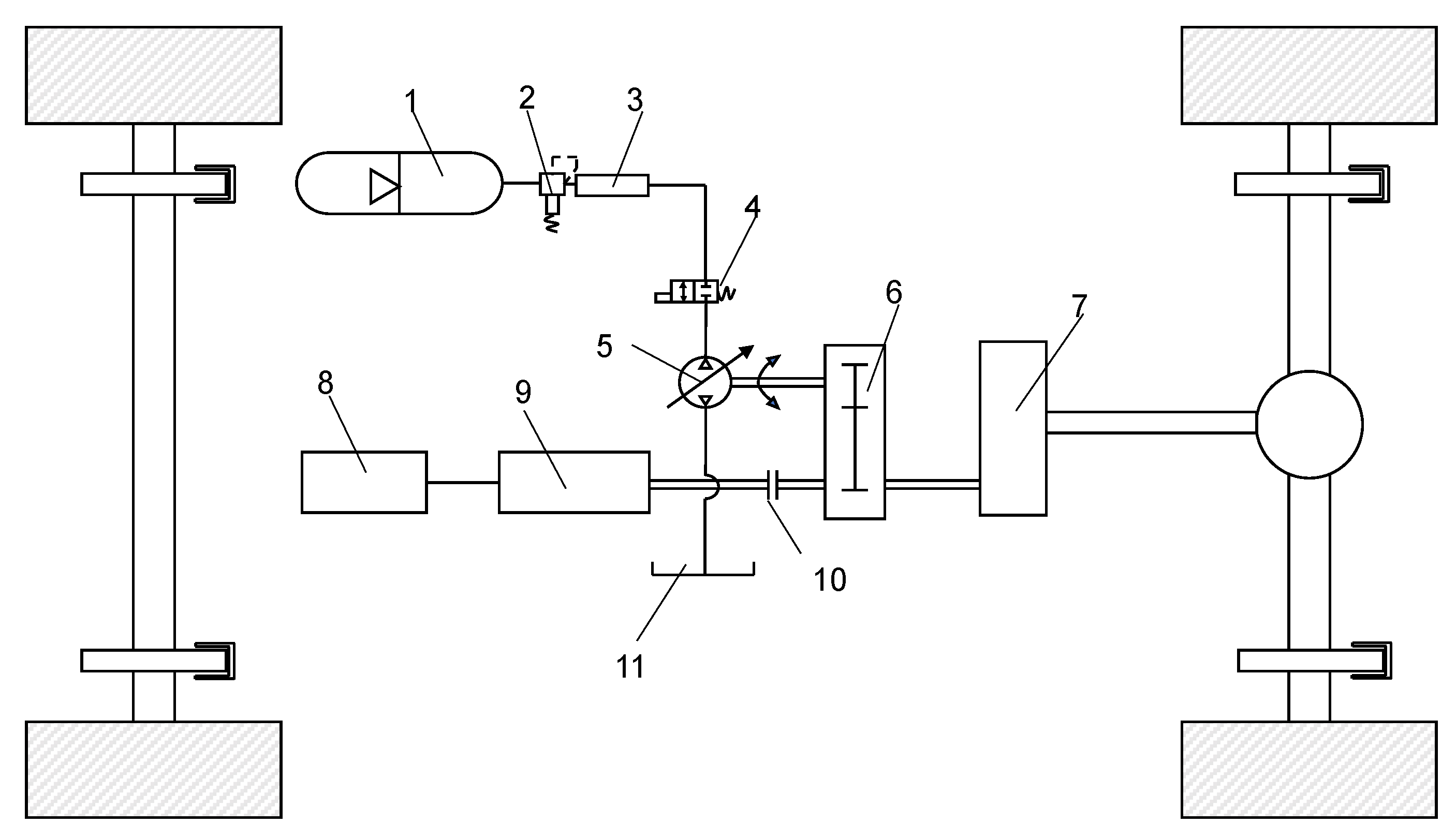
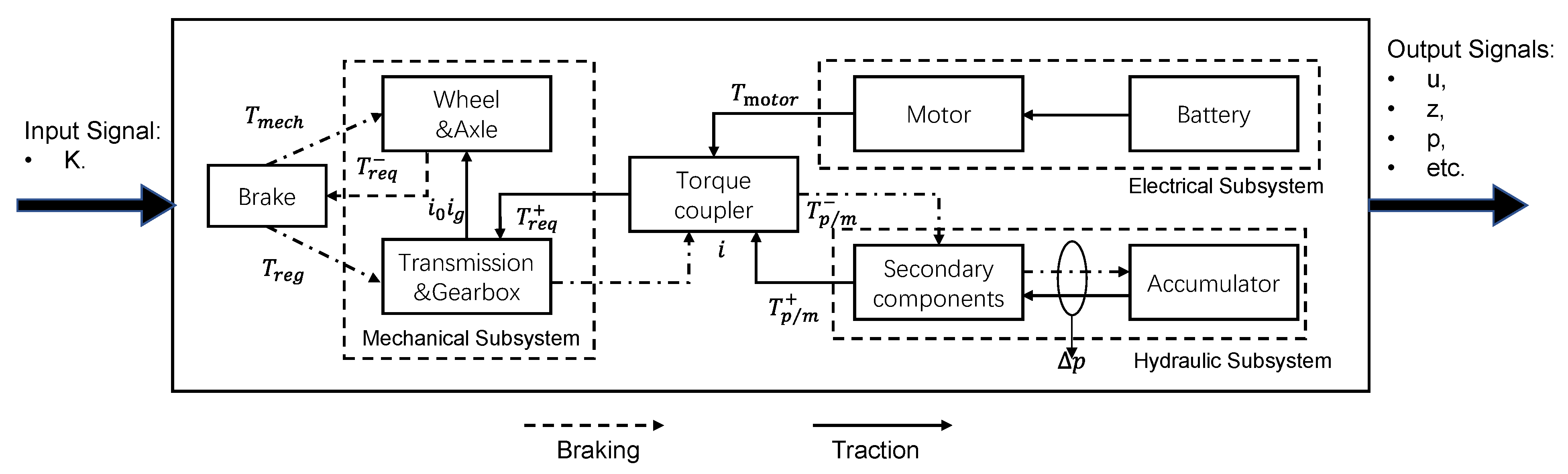
The considered hydraulic braking energy recovery system is a parallel hydraulic hybrid system (PHHS) consisting of a battery, an electric motor, a secondary component, a hydraulic accumulator, a clutch, and a torque coupling. By using the torque coupler to match the torque and speed, the torque is transmitted to the gearbox, the final reducer, and finally the wheels (Figure 1). Secondary components and hydraulic accumulators are used to recover the braking energy. Since the two power systems, namely the electric drive and hydraulic drive, are connected in parallel, the parallel hybrid vehicle has multiple operating modes, including a pure electric drive mode, pure hydraulic drive mode, and hybrid drive mode.

The motor output torque and the hydraulic system output torque of the two-axis parallel structure are connected through a torque coupler. Since the motor and the secondary components are on two separate drive shafts, the electric system and the hydraulic system can output torque independently, ignore the influence of speed and operate independently in their respective high-efficiency zones, and make it easy to match the two power sources. At this time, since the double-shaft parallel structure is relatively simple, there are fewer energy transmission levels, which reduces the energy loss in the mechanical transmission process.

During the vehicle braking process, the secondary component works as a hydraulic pump that converts the kinetic energy into hydraulic energy, and then this energy is stored in the accumulator. During the vehicle starting and hill climbing processes, the secondary component acts as a motor, releasing the energy stored in the accumulator to drive the vehicle. When the hydraulic accumulator is unable to provide the torque in the drive phase, the electric motor will participate instead. During daily driving, the hydraulic system also participates in providing torque when the motor output torque is insufficient.

In the HRBS, the secondary component has both energy storage and driving functions. The torque provided by the secondary component is calculated as follows $\left(\mathrm{N}\cdot \mathrm{m}\right)$ [28]:

$$T_{p/m}=\frac{\Delta p{q}_{p/m}{\eta }_{p/m}{i}_0{i}_{g}i}{2\pi }$$

(1)

where $\Delta p$ is the amount of accumulator pressure change $\left(\mathrm{Mpa}\right)$, $q_{p/m}$ is the displacement of the hydraulic pump motor $\left(\mathrm{mL}/\mathrm{r}\right)$, ${\eta }_{p/m}$ is the mechanical efficiency of the secondary component, $i_0$ is the torque coupling ratio, $i_g$ is the speed ratio of the gearbox, and $i$ is the speed ratio of the final drive.

The braking force required to brake the vehicle is expressed as:

$$T_{req}=\left\{\begin{array}{l}{T}_{req}^{+}=T_{motor}+T_{p/m}^{+}\hspace{1em}\hspace{1em}\hspace{1em}\hspace{1em}\hspace{1em}\hspace{1em}\hspace{0.17em}\hspace{0.17em}(traction)\\ T_{req}^{-}=T_{mech}+T_{reg}=T_{mech}+T_{p/m}^{-}\hspace{0.33em}\hspace{1em}(braking)\hspace{0.33em}\end{array}\right.$$

(2)

where $T_{motor}$ is the driving force provided for the motor, $T_{p/m}^{+}$ is the driving force provided by the secondary component, $T_{mech}$ is the mechanical friction braking force, and $T_{p/m}^{-}$ is the braking force provided by the secondary component.

The main parameters of the hydraulic accumulator include the initial pressure, volume, displacement, and maximum working pressure. In the hydraulic system, when the initial pressure of the accumulator is high, the braking torque and energy recovery efficiency provided by the HRBS will also be high, but the maximum energy absorbed will be reduced. The smaller the volume of the accumulator, the faster the accumulator pressure rises during braking, the greater the regenerative braking torque, and the higher the regenerative braking efficiency, but this will also cause the same energy storage capacity problem. In consideration of the airtightness and safety of the accumulator, the maximum pressure of the accumulator is usually 31.5 Mpa. According to Boyle’s law:

$$P_0{V}_0{}^n=P_1{V}_1{}^n=P_2{V}_2{}^n=const$$

(3)

During braking, the energy recovered by the hydraulic accumulator is calculated as:

$$E_{reg}=\frac{P_1{V}_1}{n-1}\left[{\left(\frac{P_1}{p}\right)}^{\frac{1-n}{n}}-1\right]$$

(4)

where $P_0$ is the initial inflation pressure, $V_0$ is the initial volume of the accumulator, $P_1$ is the minimum working pressure, $V_1$ is the minimum working volume, $P_2$ is the maximum working pressure of the accumulator, and $E_{reg}$ denotes the maximum energy that can be stored in the accumulator (when $p=P_2$).

The kinetic energy of the vehicle is selected as the main objective in braking energy recovery, which is simplified as follows:

$$E_{acc}=\frac{1}{2}m{u}_0{}^2-\frac{1}{2}m{u}_1{}^2$$

(5)

where $m$ is the mass of vehicle, $u_0$ is the speed of the vehicle before braking, and $u_1$ is the speed of the vehicle at the end of the braking phase.

The braking energy recovery efficiency can be expressed as follows:

$$\eta =\frac{E_{reg}}{E_{acc}}$$

(6)

Combined with the operating characteristics of the PHHS, the secondary component needs to meet the following requirements: (1) in the starting phase of the vehicle, the hydraulic system can drive the vehicle independently, i.e., the hydraulic system’s output torque is greater than the vehicle’s demand torque; (2) in the braking phase, the hydraulic pump needs to provide as much regenerative braking force as possible to improve the efficiency of the braking energy recovery.

To meet the requirements of the starting phase, the torque provided by the hydraulic motor needs to be greater than the combined force of the rolling resistance, aerodynamics resistance, and slope resistance. Therefore, the motor displacement needs to satisfy the following equation:

$$q_{p/m}\ge \frac{2\pi rF}{\Delta p{\eta }_{p/m}{i}_0{i}_g{\eta }_M}$$

(7)

$$F=mgf\cos \alpha +mg\sin \alpha +\frac{\rho C_{D}A{u}^2}{2}$$

(8)

where ${\eta }_M$ is the total mechanical efficiency, $r$ is the wheel radius, $g$ is the gravitational constant, $F$ is the sum of the vehicle driving resistance, $f$ is the rolling resistance coefficient, $\alpha$ is the ground inclination angle, $\rho$ is the density of air, $C_D$ is the aerodynamics resistance coefficient, and $A$ is the front area of the vehicle.

In pursuit of maximum energy recovery efficiency, the HRBS needs to meet the light braking conditions for all braking forces provided by the hydraulic pump; when the braking strength is 0.1 (braking strength is defined as the ratio of deceleration to gravitational acceleration), the hydraulic pump displacement needs to meet:

$$q_{p/m}\ge \frac{2\pi rmgz}{\Delta p{\eta }_{p/m}{i}_0{i}_g{\eta }_M}$$

(9)

where $z$ is the braking strength.

When the stored energy of the energy storage system reaches its limit, it is unable to receive the recovered energy from the outside world and cannot effectively deliver the required braking torque of the vehicle. In some braking situations, the increased braking force of the HRBS cannot fully provide the required braking torque for the vehicle, so friction braking is required in the achieving braking process. The total braking force of the vehicle consists of the front and rear braking forces:

$$F_{\mathrm{car}}=F_{front}+F_{rear}=fmg$$

(10)

where $F_{front}$ consists of mechanical braking and regenerative braking, and $F_{rear}$ consists of mechanical braking only. During vehicle braking, the braking effect is related to the utilization rate of the road attachment conditions.

When the adhesion conditions are not fully utilized, the vehicle is likely to slide sideways or show braking instability. When the front and rear axles of the car are clutched, the utilization rate of the road adhesion conditions is the highest, and the stability of the vehicle when braking is also the best. Therefore, when both the front and rear axles are locked:

$$F_{front}=\frac{fmg\left(b+z{h}_g\right)}{L}$$

(11)

$$F_{rear}=\frac{fmg\left(a-z{h}_g\right)}{L}$$

(12)

where $a$ is the horizontal distance from the center of mass of the vehicle to the front axle, $b$ is the horizontal distance from the center of mass of the vehicle to the rear axle, $L$ is the wheelbase of the vehicle, and $h_g$ is the height of the center of mass of the vehicle.

For each possible coefficient of adhesion, the following method can be used to obtain the front wheel braking force with the front and rear wheels locked simultaneously:

$$F_{front}=\frac{1}{2}\left[\frac{mg}{h_g}\sqrt{a^2-\frac{4h_{g}L}{mg}{F}_{rear}}-\left(2F_{rear}-\frac{mga}{h_g}\right)\right]$$

(13)

The regenerative braking factor $K$ proposed in the HRBS is defined as the braking force provided by the hydraulic pump divided by the demanded braking torque of the front wheel:

$$K=\frac{T_{p/m}/r}{F_f}$$

(14)

The regenerative braking distribution strategy is based on safety, first through the distribution of the front and rear axle braking torque so that the vehicle brake safely, and then in the form of a combined regenerative and mechanical braking distribution in the front axle.

3. FQL Algorithm and Models

A large number of researchers have introduced fuzzy control theory to the vehicle control process and achieved some results, but fuzzy control still relies on expert experience, and for some nonlinear systems, fuzzy control cannot achieve optimal control results [29]. In addition, once a fuzzy controller has been designed and produced, the vehicle equipped with the controller will follow this control rule in all operating conditions, leading to neglect of some of the recoverable energy.

Therefore, to solve the problem whereby fuzzy control cannot handle complex nonlinear systems, we introduce reinforcement learning algorithms and adjust the fuzzy rules of the fuzzy controller using the Q-Learning algorithm. In our proposed controller, the FQL algorithm acts as a decision engine that learns approaches to map the input states to the desired output decisions. The controller can maintain the original expert experience, while the FQL has an exploration function that improves the braking energy recovery performance.

The Q-learning algorithm is a table-driven learning algorithm. On the one hand, the use of fuzzy logic can solve the computational capacity limit and storage problems of Q-learning in the face of large-scale continuous state action problems, and fuzzy logic can improve the generalization ability of the reinforcement learning state action space. On the other hand, the FQL can optimize the control effect of the controller. Therefore, the FQL algorithm makes up for the shortcomings of fuzzy control and Q-learning algorithms.

3.1. FQL Model

The Markov decision process is the basic model of reinforcement learning. To solve a specific learning task, an agent is placed in an unknown environment, the agent takes an action based on the state in the environment, and the action can change its state in the environment and return a delayed numerical reward to the agent. The goal of the agent is to learn a strategy with which to take an action that allows the agent to maximize the accumulated reward in the task. Q- learning is a popular reinforcement learning algorithm that learns knowledge by updating a Q-table through a reward mechanism. The Q value is the expected cumulative reward that can be obtained by following the optimal policy after taking a certain action in each state. After learning, the agent is able to construct an optimal policy by simply selecting the action with the highest Q value in each state. The RL problem is modeled as follows:

• $X=\left\{{\mathrm{x}}^1,\hspace{0.33em}\dots \hspace{0.33em},x^n,\hspace{0.33em}\dots \hspace{0.33em},x^N\right\}$ is the set of all environment states, $x_t\in X$ indicates the state of the agent at the moment $t$;
• $O=\left\{o^1,\hspace{0.33em}\dots \hspace{0.33em},o^n,\hspace{0.33em}\dots \hspace{0.33em},o^N\right\}$ is the set of all actions that the controlled object can perform, and $u_t\in U$ indicates the actions performed by the agent at the moment $t$;
• $r_t$ is a scalar quantity indicating that the object of the controlled pair is under the state $x_t$, where at this time action $u_t$ is taken and the environmental state shifts to $x_{t+1}$, at which time the controlled object gets an immediate reward;
• The Q value corresponding to each state action is updated by the temporal difference (TD) method with the following rules:

  $$Q_{t+1}\left(x_t,a_t\right)\hspace{0.33em}=\hspace{0.33em}{Q}_t\left(x_t,a_t\right)+\beta \left[r_{t+1}+\gamma {\max }_{a^{\prime }}{Q}_t\left(x_t,a^{\prime }\right)-Q_t\left(x_t,a_t\right)\right]$$

  (15)

Here, $r_{t+1}$ is the observed reward, $\beta$ is the learning rate, and 0 ≤ $\beta$ ≤ 1. High values of $\beta$ result in rapid learning and adaptation, while low values of $\beta$ slow down the learning and prevent the impact on the q-table from possible outliers. The ${\max }_{a^{\prime }}{Q}_t\left(x_t,a^{\prime }\right)$ denotes the state $x_t$ of the estimated optimal value of Q under the discount factor $\gamma$, 0 ≤ $\gamma$ ≤ 1. The value of $\gamma$ determines whether the optimization process should consider the long-term reward or not.

Q-learning is not good at dealing with situations where the state space is relatively large, since a large amount of memory is needed to store the q-table. Even if a large amount of memory can be provided, agent learning requires a lot of trials and time to learn the required behavior, and vehicles driving urban routes require different environments to satisfy q-table updates in all cases, thereby causing a lot of learning costs.

FQL is a fuzzy extension of Q-learning that can overcome this problem [30]. We can encapsulate expert knowledge into a learning table to speed up the learning process. In FQL, the decision part is represented by a fuzzy inference system (FIS), which takes continuous and large discrete states as the inputs. The idea of the FQL algorithm is to use the FIS to integrate continuous and large discrete state inputs into a so-called q-table, which is different from the original q-table; the new q-table is based on evaluating the fuzzy rules in the FIS as the basis for updating the q-table. Compared to the infinite action- state space, fuzzy rules are finite and are used as inputs to the q-table so that the q-table can learn knowledge without relying on large amounts of memory.

In FQL, the FIS is represented by a set of fuzzy rules $J$. Rule $j$ ∈ $J$ is defined as:

$$\begin{array}{c}IF\left(x^1\hspace{0.33em}is\hspace{0.33em}{L}_j^1\right)\dots AND\left(x^n\hspace{0.33em}is\hspace{0.33em}{L}_{\mathrm{j}}^n\right)\dots AND\left(x^{\mathrm{N}}\hspace{0.33em}is\hspace{0.33em}{L}_{\mathrm{j}}^{\mathrm{N}}\right)\\ \hspace{0.33em}THEN\hspace{0.33em}a\hspace{0.33em}=\hspace{0.33em}{o}_j\hspace{0.33em}with\hspace{0.33em}\mathrm{q}\left(L_{\mathrm{j}},o_j\right)\end{array}$$

(16)

where $L_j^n$ is the label of the input variable $x^n$ base on rule $j^{th}$, $o_j$ is the action of the rule $j^{th}$,$L_j=\left\{L_j^1,\hspace{0.33em}\dots \hspace{0.33em},L_j^n,\hspace{0.33em}\dots \hspace{0.33em},L_j^N\hspace{0.33em}\right\}$ is the modal vector under rule $j$, and $q\left(L_j,o_j^k\right)$ is the modal vector $L_j$ and the action $o_j^k$ of rule $j^{th}$ in the Q value.

In the fuzzification layer of the FIS (Figure 2), the input states are fuzzified into the affiliation degree of the corresponding label by the affiliation function, and each input state is fuzzified to obtain a fuzzy set ${\mu }_L^n=\left\{{\mu }_1\left(x^n\right),\hspace{0.33em}\dots \hspace{0.33em},{\mu }_n\left(x^n\right),\hspace{0.33em}\dots \hspace{0.33em},{\mu }_N\left(x^n\right)\right\}$. Let $J_x$ denote the set of all rules in the rule evaluation layer, and each rule is a scalar obtained by multiplying the fuzzy sets corresponding to the input states, then the set of rules is the Cartesian product of the fuzzy sets corresponding to the input states. For the rules $j^{th}$ ($j^{th}\in J$), $\alpha$ denotes the activation degree of this rule, which can be expressed as follows:

$${\alpha }_j\left(x\right)\hspace{0.33em}=\hspace{0.33em}{\displaystyle \prod _{n=1}^{\mathrm{N}}{u}_{L_j}^n\left(x^n\right)}$$

(17)

In the FQL algorithm, we take a two-stage action selection approach. In the first stage, we select the local action according to the $\epsilon -greedy$ strategy to select local actions $o_j^l$. The agent makes it possible to explore untried actions instead of the action with the largest Q value, in order to ensure a higher long-term payoff. At each time step, the agent selects random actions with a fixed probability of $1-\epsilon$. At the beginning of the exploration, we let the agent take more random actions instead of greedily choosing the optimal action in the q-table.

$$\left\{\begin{array}{l}\hspace{0.33em}\epsilon \forall j\in J_x:o_j^l\hspace{0.33em}=\arg \max x_{k\in K}q\left(L_j,o_j^k\right)\\ 1-\epsilon \forall j\in J_x:o_j^l\hspace{0.33em}=\mathrm{random}{x}_{k\in K}(o_j^k)\end{array}\right.$$

(18)

where $o_j^k$ is the local action of the rule $j^{th}$. In the second stage of the action selection, the activation degree of the rule is obtained according to the input state, and the activation degree multiplied by the local action can be used to obtain the final action; here, the agent chooses the final action with the highest activation degree of the rule; then the final action output can be expressed as:

$$a={\max }_{j\in J_x}{\alpha }_j\left(x\right)o_j^l$$

(19)

By adding the time index to the equation, the Q value can be approximated as:

$$Q\left(x_t,a\right)={\displaystyle \sum _{j\in J_x}{\alpha }_j\left(x_t\right)\hspace{0.33em}\times \hspace{0.33em}q\left(L_j,o_j^l\right)}$$

(20)

After taking action, the agent obtains the status $x_{t+1}$ and reward $r_{t+1}$. Then, the state $x_{t+1}$ of the Q value is calculated as follows:

$$V\left(x_{t+1}\right)={\displaystyle \sum _{j\in J_{x+1}}{\alpha }_j\left(x_t\right)\hspace{0.33em}\times \hspace{0.33em}\underset{k}{\max }\left(L_j,o_j^k\right)}$$

(21)

Based on the above equation, the error is calculated by the TD algorithm as follows [31]:

$$\Delta Q=r_{t+1}+\gamma V\left(x_{t+1}\right)-Q\left(x_t,a\right)$$

(22)

Ultimately, we can update the Q value of each activation rule by using the above equation as follows:

$$q_{t+1}\left(L_j,o_j^l\right)=q_t\left(L_j,o_j^l\right)+\beta {\alpha }_j\left(x_t\right)\Delta Q$$

(23)

where $\gamma$ and $\beta$ are the same as in Equation (15).

3.2. Regenerative Braking Based on FQL

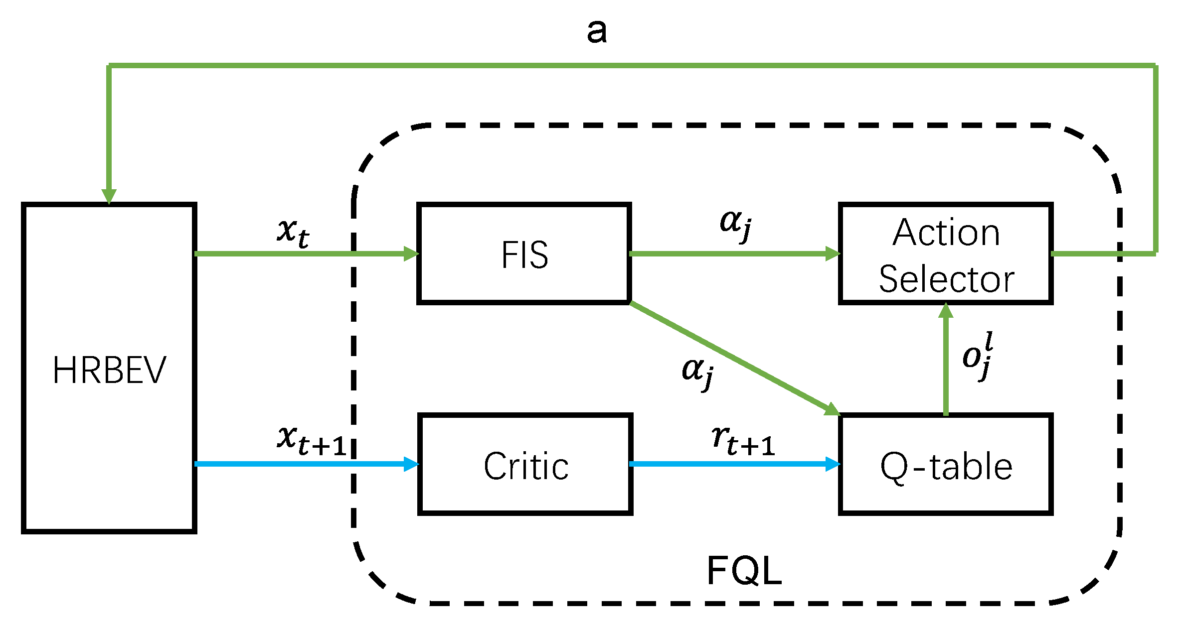
In this section, the above fuzzy reinforcement learning model will be simulated jointly with the regenerative braking system for electric vehicles. Here, the HRBS for the electric vehicles (HRBEV) is built in MATLAB and Simulink, which will be introduced later. The FQL model is built in Python and simulated jointly with Python and MATLAB. At each time step, the HBREV outputs state $x_t$ as the input of the FQL, which is fuzzed in the FIS. Then, the optimal action is selected according to the fuzzy rules and q-table, and the agent outputs action $a$ to the HRBEV. In the next time step, the state $x_{t+1}$ is output to the FQL model from the HRBEV. The critic gives $r_{t+1}$ from $x_{t+1}$. Finally, the q-table is updated using the TD method (Figure 3).

3.2.1. FQL Components

The RBFQL consists of the HRBEV and FQL, and the FQL consists of the following components.

• State: The input state consists of the vehicle speed, braking intensity, accumulator pressure, demand braking torque, hydraulic pump providing torque, and other components. Here, the vehicle speed, braking intensity, and pressure of the accumulator are used as inputs of the FIS, while other components are used as inputs to the FQL observation reward value:

$$x_t=\left\{u,z,p\right\}$$

(24)

where $u$ denotes the vehicle speed, $z$ denotes the braking intensity, and $p$ is the accumulator pressure.

• Action: The output action is the regenerative braking coefficient. The brake distribution factor needs to meet the vehicle braking safety and reduce the output when the accumulator is full:

$$a=\left\{{\alpha }_j{o}_j^1,{\alpha }_j{o}_j^2,\hspace{0.33em}\dots \hspace{0.33em},{\alpha }_j{o}_j^n\right\}$$

(25)

• Reward function: The design of the reward function is the key to building a reinforcement learning system. The agent gets a reward based on the observed state and uses the reward to update the q-table. The goal of reinforcement learning is to maximize the cumulative reward over time, and the agent seeks to produce the action with the maximum Q value. In our system, the reinforcement learning goal is to seek to maximize the regenerative braking energy. Therefore, our reward function can be expressed as:

$$r_{t+1}=\left(1-\frac{u_{t+1}}{u_{req}}\right)+\frac{\Delta p}{P_{\max }-P_0}$$

(26)

where $u_{req}$ is the required speed at time $t+1$ and $u_{t+1}$ is the real vehicle speed at time $t+1$, $\Delta p$ is the accumulator pressure change under braking conditions, $P_{\max }$ is the maximum pressure of the accumulator (31.5 Mpa here), and $P_0$ is the minimum working pressure of the accumulator. Obviously, to obtain a larger reward, it is necessary to make the real vehicle speed $u_{t+1}$ as small as possible and the accumulator pressure variation as large as possible. If the reward is close to 0, this means that the action is invalid, and a negative reward means a penalty for the action. For example, if the agent takes an aggressive action in a certain state, i.e., takes a larger regenerative braking factor, the accumulator pressure change becomes large, and a large reward is obtained. However, due to the torque limitation of the pump, the pump does not provide enough braking torque, which will result in the $\frac{u_{t+1}}{u_{req}}$ being large, and the penalty will increase at this time. Therefore, the method for dealing with the relationship between the reward and punishment is the key to reinforcement learning.

3.2.2. Fuzzy Inference System

In this paper, we simulate the vehicle dynamics model in urban cyclic conditions (1015 cycle and UDDS cycle). Due to the limitation of the vehicle′s operating environment, it is not possible for all action states to be traversed, but we need the agent to output a more appropriate action even when facing an inexperienced environment. Therefore, we choose the fuzzy control approach to add knowledge to the action selection process in the form of rules, which can improve the speed of the agent in dealing with complex continuous state spaces or multidimensional discrete spaces [32].

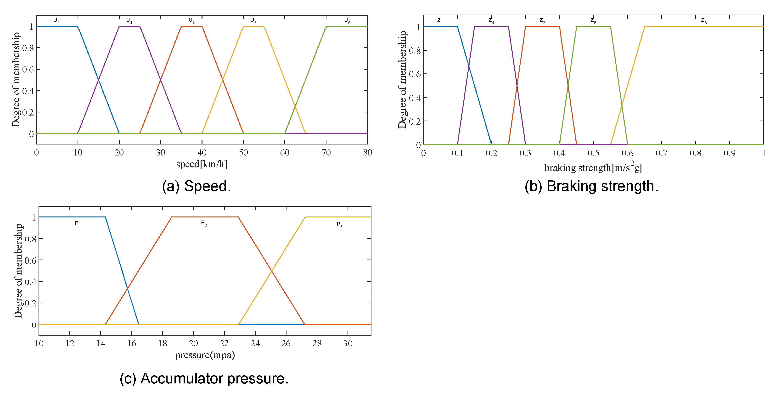
The FQL system inputs three input variables: (1) vehicle speed $u$, (2) braking intensity $z$, and (3) accumulator pressure $p$; and one output—(4) regenerative braking distribution coefficient $k$. The fuzzy division of these four variables is as follows:

• The vehicle speed $\left(u\right)$. $T_u=\left\{U_1,\hspace{0.33em}\dots \hspace{0.33em},U_5\right\}$, and the range of the theoretical domain is (0–80) ( $\mathrm{km}/\mathrm{h}$ );
• The braking strength $\left(z\right)$. $T_z=\left\{Z_1,\hspace{0.33em}\dots \hspace{0.33em},Z_5\right\}$, and the theoretical domain range is (0–1) ( $\mathrm{m}/{\mathrm{s}}^2\mathrm{g}$ );
• The hydraulic accumulator pressure $\left(p\right)$. $T_p=\left\{P_1,\hspace{0.33em}{P}_2,P_3\right\}$, and the theoretical domain range is (10–31.5) ( $\mathrm{Mpa}$ );
• The regenerative braking coefficient $\left(k\right)$. $T_k\left\{K_1,\hspace{0.33em}\dots \hspace{0.33em},K_5\right\}$, and the theoretical domain range is (0–1).

The Sugeno method has the advantage of allowing simple calculations and facilitating data analyses, so we chose to set up the fuzzy control system using the first-order Sugeno method. The fuzzy control system performs the fuzzy inference process using fuzzy rules to obtain the output under different operating conditions. The knowledge base of the fuzzy system is described by a series of fuzzy logic rules in the form of IF–THEN, and the fuzzy rules are used as follows:

$$IF\hspace{0.33em}u\hspace{0.33em}is\hspace{0.33em}{U}_i\hspace{0.33em}AND\hspace{0.33em}z\hspace{0.33em}is\hspace{0.33em}{Z}_l\hspace{0.33em}AND\hspace{0.33em}p\hspace{0.33em}is\hspace{0.33em}{P}_m\hspace{0.33em}THEN\hspace{0.33em}k\hspace{0.33em}is\hspace{0.33em}{K}_n$$

(27)

where $U_i\in T_i,i=1,2,3,4,5$, $Z_l\in T_z,l=1,2,3,4,5$, and $P_m\in T_p,m=1,2,3$. The regenerative braking coefficient $T_k=\left\{K_1,\hspace{0.33em}{K}_2,K_3,\hspace{0.33em}{K}_4,K_5\right\}=\left\{0,0.25,0.5,0.75,1\right\}$ (Figure 4). For example, when the vehicle speed is very low, the braking intensity is medium, and the accumulator pressure is very low, the regenerative braking distribution coefficient will be very high. When the vehicle speed is high, the braking intensity will be high, and the accumulator pressure is medium, the regenerative braking distribution coefficient will be very low. The idea of the rule set is to try to recover more energy at low speeds and ensure safety at high speeds, and regenerative braking is not involved in the work. The total number of rules in the rule set is $75\left(5\times 5\times 3\right)$.

The FIS will be improved using the QL method to obtain better performance.

3.2.3. FQL Setup

In the FQL setup, we will set the discount factor through the phasing $\gamma$, learning rate $\beta$, and random action selection probability $1-\epsilon$. In the early stage of learning and the exploration stage, we set the discount factor $\gamma$ to 0.2, because in the early stage of training, $Q\left(s\right)$ and $V\left(s\right)$ do not converge, meaning the agent cannot correctly measure the expected future benefits. A higher discount factor will cause the agent to incorrectly estimate the current action value, leading to instability when the algorithm is updated, even making it difficult to converge. The discount factor will gradually increase as the training process proceeds. Meanwhile, we set the learning rate $\beta$ value to 0.9, as a larger learning rate at the early stage of learning can reduce the training time, and the subsequent reduction in the learning rate is beneficial to maintaining the system stability. The probability of random action selection in the exploration phase $1-\epsilon$ is set to 0.5; the agent needs to balance the maximum value action and develop potential higher value actions, while the random action selection probability will decrease with the learning process. Here, we compare the regenerative braking system with the fuzzy controller without adding the QL algorithm, so that we can judge the learning process and modify the above parameters. In addition, we initialize the q-table to zero to start the knowledge learning process from zero.

So far, this paper has completed the modeling of the hydraulic parallel hybrid braking system and vehicle dynamics, combined with the FQL to model the vehicle regenerative braking problem. The next section will verify the above system and the simulation of vehicle braking efficiency through experimental and simulation comparison methods.

4. Experiment and Simulation Results

In this section, we will apply the method proposed above for vehicle regenerative braking energy recovery in three steps. First, we build a test bench and the above mathematical model in Simulink to compare the test and simulation results. Then, we integrate the obtained Simulink model into the ADVISOR environment to model the regenerative braking torque distribution through fuzzy control. Finally, we use MATLAB API engine to simulate ADVISOR in parallel with the fuzzy reinforcement learning algorithm in Python to validate the proposed method.

4.1. Experiment Test

The experimental platform is built based on the PHHS established in the previous paper. The difference from Figure 1 is that we use the flywheel moment of inertia to simulate the kinetic energy of the vehicle to study the energy recovery efficiency of the hydraulic system. The kinetic energy simulation part consists of the flywheel, magnetic powder brake, electromagnetic clutch, three-phase synchronous motor, inverter, and console. Among them, the magnetic powder brake is used to simulate the mechanical friction brake, the electromagnetic clutch is used to open and close the direct connection between the motor and the flywheel, the motor provides the initial kinetic energy of the flywheel, the inverter is used to control the motor and adjust its speed, and the console controls the engagement of the electromagnetic clutch and the switch of the inverter (Figure 5). The hydraulic brake energy recovery part mainly consists of the secondary component, a hydraulic accumulator, and an oil tank. The secondary component converts the kinetic energy of flywheel rotation into hydraulic potential energy and fills the hydraulic accumulator with liquid. The hydraulic accumulator is the energy storage element, and the hydraulic oil is supplied from the oil tank. In addition to the above components, a speed sensor, voltage sensor, current sensor, pressure sensor, electrical parameter tester, and acquisition card are required to collect the experimental data.

Table 1. Main component parameters of the kinetic energy simulation part.

Name	Model	Key Parameters
Motor	Y132S-4	Rated speed: 1440 r/min Rated voltage: 380 V Maximum power: 5.5 KW
Flywheel		Rotational inertia: 45.3 $\mathrm{kg}\cdot {\mathrm{m}}^2$
Secondary Component	Secondary Component	Maximum Displacement: 107 mL/r Minimum Displacement: 38 mL/r
Hydraulic Accumulator	NXQ	Nominal volume: 25 L Nominal pressure: 31.5 MPa
Voltage Sensor	MIK-DZU-100V	Measuring range: 0~100 V Output: 0~10 V
Current Sensor	MIK-DZI-150A	Measuring range: 0~150 A Output: 0~10 V
Pressure sensors	MCY-X	Measuring range: 0~35 MPa Sensitivity: 2 MPa/V
Photoelectric speed sensor	DK890	Operating voltage: 10~36 V Measurement range: 0~10 kHz
Acquisition Cards	USB3103A	Signal channels: 16 Sampling frequency: 500 kHz

shows the parameters of each component of the experimental stand.

In the bench experiment, the flywheel starts braking when the hydraulic pump starts working. The kinetic energy possessed by the flywheel is expressed as:

$$E_f=\frac{1}{2}J{\omega }^2$$

(28)

We performed three different sets of experiments based on the above experimental bench. By comparing the experimental data with the simulation data, we verified the accuracy of our simulation model. The simulation model will be used as the basis of the proposed algorithm.

First of all, we performed experiments and simulations with different initial flywheel speeds (Figure 6a). Here, the initial pressure of the accumulator is set to 5.6 MPa; the volume of the accumulator is 25 L; the displacement of the hydraulic pump is 50 mL/r; and the flywheel speeds are 360 r/min, 300 r/min, and 240 r/min when the electromagnetic clutch starts to close, and the flywheel drives the oil pump to rotate. It can be found that the rising trend of experimental and simulated accumulator pressures are almost the same, and the error is approximately 10%. In the experimental results, because the energy consumed by the friction will increase with the increase in speed of the flywheel, the energy recovery efficiency will decrease. Additionally, higher flywheel speeds can achieve higher energy recovery rates in the hydraulic regeneration system. The difference between the experimental and simulated response times is caused by the hydraulic system needing a response time of about 0.7 s, but the results of experiments and simulations will be basically unchanged.

To find the energy recovery efficiency of the braking process, the braking energy recovery efficiencies at different initial speeds can be calculated according to Equations (5) and (28), as shown in

Table 2. Final pressure and energy recovery efficiency of the accumulator at various speeds.

Component	Description	240 r/min	300 r/min	360 r/min
Experimental results	pressure	6.45 MPa	6.79 MPa	7.23 MPa
	efficiency	84.96%	85.7%	85.97%
Experimental results	pressure	6.25 MPa	6.62 MPa	7.05 MPa
	efficiency	78.05%	76.65%	74.01%

.

Secondly, we performed experiments and simulations with different initial accumulator pressures (Figure 6b). Here, the initial speed of the flywheel is 300 r/min; the displacement of the hydraulic pump is 50 mL/r; the initial volume of the accumulator is 10 L; and the initial pressures of the accumulator are 4.5 MPa, 5 Mpa, and 5.6 MPa. It can be found that an accumulator with a high initial pressure will also have a high final pressure after the same braking process. The experimental results will be slightly lower than the simulation results.

Thirdly, we performed experiments and simulations with respect to flywheel speeds with different initial accumulator pressures (Figure 6c). It can be observed from the results that the larger the initial accumulator pressure, the shorter the braking process time and the larger the power of the hydraulic regeneration system to provide recovery energy.

For the trend of the three sets of experiments, it can be found that the greater the accumulator instantaneous pressure, the greater the power of the hydraulic regeneration system to provide recovery energy, and more braking energy can be recovered. The experimental flywheel deceleration time is smaller than the simulated one, which is caused by the existence of larger friction in the system.

Regarding the effect of the initial pressure of the accumulator on the braking energy recovery efficiency, the simulation and experimental results are shown in

Table 3. Final pressure and energy recovery efficiency rates of the accumulator at various initial pressures.

Component	Description	4.5 MPa	5 MPa	5.6 MPa
Experimental results	pressure	6.78 MPa	7.23 MPa	7.81 MPa
	efficiency	80.3%	85.7%	81.2%
Experimental results	pressure	5.91 MPa	6.51 MPa	7.56 MPa
	efficiency	70.55%	73.65%	72.01%

.

The displacement of the accumulator affects the volume change in the accumulator oil and the output torque per unit of time. Here, we set the flywheel speed to 360 rpm; the accumulator volume is 16 L; the initial accumulator pressure is 5.7 MPa; and the hydraulic pump displacement rates are 60 mL/r, 50 mL/r, and 38 mL/r for the experiment (Figure 7).

From the experimental and simulation results, it can be seen that with larger displacement rates of the hydraulic pump, the braking torque output by the hydraulic pump increases rapidly, and the accumulator pressure rises rapidly at the early stage of braking. During the later stage, the braking torque output by the hydraulic pump tends to level off and the accumulator pressure rises slowly, then the pressure of the accumulator is consistent finally. Therefore, the simulation and experimental results generally tend to be consistent, and the simulation model has good accuracy.

4.2. Simulation Results

The vehicle model is based on the ADVISOR pure electric vehicle model for secondary development. A pure electric vehicle is selected in the ADVISOR module library, and its model parameters are modified according to a pure electric bus developed by a bus company. Here, we add the above hydraulic regenerative braking simulation model, modify the original vehicle control strategy, and train the FQL algorithm. Figure 8 shows the torque transfer diagram of the HRBS. Figure 9 shows how we combined the electric vehicle HRBS model in the ADVISOR environment. In addition, according to the characteristics of the frequent starting and stopping of urban buses, the simulation environments for the 1015 cycle and UDDS cycle are selected, including the acceleration, deceleration, uniform speed, uphill and downhill conditions, and other working conditions, as shown in Figure 10.

The hydraulic pump displacement and the transmission ratio of the torque coupler in the HRBS are selected according to the following rules. The hydraulic pump displacement is 0.025 L/r for the 1015 operating conditions and 0.03 L/r for the UDDS operating conditions. The transmission ratio for both torque couplers is 2.5. The state of charge (SOC) of the vehicle battery is set to 1 at the beginning of the simulation, and the vehicle SOC decreases as the simulation proceeds, serving as an evaluation index of the energy recovery effect.

Compared with the two driving cycles, the 1015 cycle has a low braking frequency, low intensity, and high percentage of regenerative braking forces. The UDDS cycle has a high braking frequency and high intensity, so the UDDS regenerative braking torque is higher than for the 1015 cycle (Figure 11 and Figure 12). For each braking process, the HRBS with reinforcement learning can obtain a greater final pressure rate from the accumulator, as well as greater braking energy recovery efficiency and regenerative braking torque than the HRBS with fuzzy control based on expert experience and the HRBS with the DP algorithm.

It can be seen that the HRBS with FQL saves 9.62% more power than the hydraulic braking system with fuzzy control and the DP algorithm under the 1015 conditions and 8.91% more under the UDDS conditions (

Table 4. The amount of electricity consumed.

Cycle	HRBEV with FQL	HRBEV with DP	HRBEV with Fuzzy Control	Average Growth Rate (%)
1015	0.0234	0.0259	0.0254	9.62%
UDDS	0.0651	0.0703	0.0715	8.91%

). Therefore, the FQL-algorithm-based optimization strategy is effective and can be adapted to more operating conditions for adjustment.

5. Conclusions

This paper presents an algorithm for optimizing the energy recovery efficiency of the HRBS based on FQL for an urban electro-hydraulic hybrid bus. The experimental bench of the HRBS was built to verify the simulation model and investigate the influence of the HRBS parameters on the energy recovery characteristics. The whole hydraulic regenerative braking electric vehicle model was established by integrating the Simulink model into the ADVISOR. The vehicle regenerative braking control strategy was optimized using the FQL algorithm and simulated under the 1015 cycle and UDDS cycle conditions. The results showed that the control strategy optimized by the FQL algorithm recovered more braking energy than the fuzzy control strategy based on expert experience and the DP algorithm. In addition, the control strategy based on the FQL algorithm can output actions that are more consistent with the training environment, which is more flexible than the fuzzy control method. Therefore, we verified that this method can reduce the power consumption of electric vehicles and improve the efficiency of the hydraulic regenerative braking process.