Accuracy Assessment of Charge-Mode Accelerometers Using Multivariate Regression of the Upper Bound of the Dynamic Error

Abstract

This paper presents the mathematical basis and related procedures for the regression of the upper bound of the dynamic error produced by charge-mode accelerometers. The integral-square error obtained in response to simulation signals with one constraint appearing at the input of the accelerometer is considered. Physical models of accelerometers are presented with related equations and mathematical formulae that make it possible to obtain the error and the corresponding constrained signal. Examples of the regression for predefined values of the accelerometer parameters are also discussed. The solutions presented in this paper may contribute to increasing the accuracy of the charge-mode accelerometers commonly used in energy systems. Development of the functions approximating the integral-square error for the given ranges of accelerometer parameters constitutes the original contribution of this paper.

1. Introduction

Assessment of the accuracy of charge-mode accelerometers is extremely important in areas such as mechanical science [1], navigation [2], medicine [3] and geotechnics [4], particularly because they can be used over a wide temperature range [5]. In everyday engineering practice, the accuracy of this type of accelerometer is assessed by way of calibration, by comparing its charge sensitivity with the corresponding reference values [6,7]. During a measurement experiment of this type, the operating range of the sensor is verified. The accuracy of a charge-mode accelerometer is also assessed on the basis of comparability tests, through repeated measurements of acceleration and determining the standard deviation of the obtained results [8]. It should be noted that the lower the value of this deviation is, the higher is the accuracy of the accelerometer. From the point of view of assessing the accuracy of this type of sensor, it is also important to determine the influences of temperature and electromagnetic interference on the results for the corresponding charge sensitivity [9,10].

However, the abovementioned research procedures do not provide specific numerical indicators that allow for the assessment of the dynamic accuracy of charge-mode accelerometers in a way similar to the accuracy class used in static measurements [11,12]. It is possible to obtain such an indicator through simulations, by determining the upper bound of the dynamic error for an error functional assumed in advance, e.g., the integral-square error commonly used in measurements [13]. In this case, the upper bound of the dynamic error is determined as a response to a previously determined input signal with magnitude and time constraints [14]. This signal has a rectangular shape, and the number of switches depends on the rate of change of the accelerometer impulse response [13,15]. The basis for determining such a signal is a mathematical model of the accelerometer, which may be presented in the form of a transfer function or a state-space representation [16,17]. This model is determined by parametric identification of the accelerometer (a practical experiment), which is usually carried out by measuring only the corresponding amplitude response or by simultaneous measurement of both frequency responses, i.e., the amplitude and phase [18,19,20]. In turn, the upper bound of the dynamic error and the constrained signal for the integral-square error are determined using a simulation experiment, by applying an iterative procedure with a predetermined number of iterations [21,22]. In this aspect, the trace alignment procedure [23], which can improve the subsequent side-channel analysis against the trace and the chromatic plasmonic-polarizer-based synapse for all-optical convolutional neural network [24], can also be used. These procedures can be evaluated by seeking higher absolute values of the accuracy and lower values for bias, in addition to reduced cognitive load by means of self-assessment by rubric and the accuracy service with a software-defined receiver for location [25,26]. The simulation procedure requires the development of an appropriate computational procedure using dedicated mathematical and computational software (e.g., MathCad 15 or MATLAB R2023b) [27,28]. It is also time-consuming, as the average calculation time may range from several minutes to even an hour, depending on the accuracy of the calculations and the assumed number of iterations [29]. In addition, these calculation procedures need to be repeated for each accelerometer tested.

In view of these difficulties in implementing simulation procedures, this paper presents a method involving multivariate regression [30,31] of the results of the upper bound of the dynamic error, which is determined for pre-established ranges of variability for two of the four parameters associated with the mathematical accelerometer model. The quantification steps referring to these two parameters are also assumed for these intervals. The sensitivity of the accelerometer and the natural frequencies of undamped vibrations are assumed as constant values. As a result of the multivariate regression, the approximating functions can be obtained [32] on the basis of which it is possible to determine the upper bound of the dynamic error using only the results of parametric identification [33,34], without the need to carry out simulation procedures. Of course, these approximation functions only reflect the error for previously assumed ranges of variability for the accelerometer parameters. These functions may therefore constitute a proposal for a mathematical computational tool dedicated to engineering applications. On this basis, an additional comparative criterion is obtained that fully reflects the dynamic properties of the charge-mode accelerometer under consideration. It should also be emphasised that the lower the numerical value of this comparative indicator is, the higher is the accuracy of the considered accelerometer.

The method presented in this paper can be used to compare accelerometers that are from different manufacturers but have similar levels of sensitivity and similar natural frequencies of undamped vibrations. Using this tool, it may be possible to select accelerometers based on their dynamic accuracy, which would certainly improve the reliability of many technological processes, and, in particular, the reliability of solutions used in the broader energy industry.

2. Materials and Methods

Let the transfer function of a charge-mode accelerometer connected with a voltage amplifier and cable be denoted by $K_{\mathrm{Qe}}\left(s\right).$ We can then write

$$\begin{gathered} K_{\mathrm{Qe}}\left(s\right)=\frac{V\left(s\right)}{s^{2}X\left(s\right)}=\frac{s\tau S_{\mathrm{m}}{S}_{\mathrm{q}}\left(2\beta {\omega }_{0}s+{\omega }_0^2\right)}{\left(s\tau +1\right)\left(s^2+2\beta {\omega }_{0}s+{\omega }_0^2\right)} \\ =S_{\mathrm{V}}\frac{\tau \left(2\beta {\omega }_0{s}^2+{\omega }_0^{2}s\right)}{\tau s^3+\left(2\tau \beta {\omega }_0+1\right)s^2+\left(\tau {\omega }_0^2+2\beta {\omega }_0\right)s+{\omega }_0^2}, \end{gathered}$$

(1)

where $S_{\mathrm{q}}=k_{\mathrm{p}}/C_{\mathrm{t}} \left[\mathrm{V}/\mathrm{N}\right]$ and $S_{\mathrm{V}}=S_{\mathrm{m}}{S}_{\mathrm{q}} \left[\mathrm{V}/\left({\mathrm{ms}}^{-2}\right)\right]$ are the charge and voltage sensitivities, respectively [15,16]. This transfer function is a third-order equation with four parameters: $S_{\mathrm{V}},$ $\tau =R_{\mathrm{t}}{C}_{\mathrm{t}}$, $\beta$ and ${\omega }_0=2\mathsf{\pi }{f}_0$ [35].

The observer canonical form of the state-space representation of Equation (1) is

$$K_{\mathrm{Qe}}\left(s\right)=C_{\mathrm{Qe}}{\left(sI-A_{\mathrm{Qe}}\right)}^{-1}{B}_{\mathrm{Qe}},$$

(2)

where $I$ is the identity matrix, and $A_{\mathrm{Qe}}, B_{\mathrm{Qe}}$ and $C_{\mathrm{Qe}}$ are represented by

$$\begin{gathered} A_{\mathrm{Qe}}=\left[\begin{array}{ccc}-\left(2\tau \beta {\omega }_0\right)/\tau & 1& 0\\ -\left(\tau {\omega }_0^2+2\beta {\omega }_0\right)/\tau & 0& 1\\ -{\omega }_0^2/\tau & 0& 0\end{array}\right], B_{\mathrm{Qe}}={\left[\begin{array}{ccc}2\beta {\omega }_0& {\omega }_0^2& 0\end{array}\right]}^T, \\ {C}_{\mathrm{Qe}}=\left[\begin{array}{ccc}1& 0& 0\end{array}\right]. \end{gathered}$$

(3)

Here, $A_{\mathrm{Qe}}\in {ℝ}^{ql},$ $B_{\mathrm{Qe}}\in {ℝ}^{qm}$ and $C_{\mathrm{Qe}}\in {ℝ}^{pn},$ are the state, input, and output matrices, and $l,$ $m,$ $p$ and $q$ are the denominator order, numerator order, number of inputs and number of outputs, respectively. The above state-space representation is in many cases an alternative to Equation (1), as it enables easier implementation of the algorithm for determining the upper bound of the dynamic error.

The parameters included in the mathematical models defined by Equations (1) and (2) are listed in Table 1.

Table 1. Parameters included in the mathematical models of a charge-mode accelerometer.

Parameter	Unit of Measure	Description
$k_{\mathrm{p}}$	$\mathrm{C}/\mathrm{N}$	Piezoelectric constant
$R_{\mathrm{t}}$	$\mathsf{\Omega }$	Total resistance of accelerometer, cable and voltage Amplifier
$C_{\mathrm{t}}$	F	Total capacitance of accelerometer, cable and voltage amplifier
$S_{\mathrm{q}}$	V/N	Charge sensitivity
$S_{\mathrm{V}}$	$\mathrm{V}/\left({\mathrm{ms}}^{-2}\right)$	Voltage sensitivity
$S_{\mathrm{m}}$	kg	Mechanical sensitivity
$\tau$	s	Time constant
$\beta$	$-$	Damping ratio
${\omega }_0$	rad/s	Pulsation of undamped natural vibrations
$f_0$	Hz	Frequency of undamped natural vibrations
$A_{\mathrm{Qe}}$	$-$	State matrix
$B_{\mathrm{Qe}}$	$-$	Input matrix
$C_{\mathrm{Qe}}$	$-$	Output matrix

The integral-square error at the output $y$ of the accelerometer is defined by the following equation:

$$E{I}_y={{\displaystyle \int }}_0^T{\left[y\left(t\right)\right]}^2\mathrm{d}t$$

(4)

And, with use of Parseval’s theorem, it has the following form:

$$\begin{gathered} E{I}_y=\frac{1}{2\mathsf{\pi }}{{\displaystyle \int }}_{-\infty }^{\infty }{\left|Y\left(\omega \right)\right|}^2\mathrm{d}\omega =\frac{1}{2\mathsf{\pi }}{{\displaystyle \int }}_{-\infty }^{\infty }{\left|X\left(\omega \right)K_d\left(\omega \right)\right|}^2\mathrm{d}\omega \\ =\frac{1}{2\mathsf{\pi }}{{\displaystyle \int }}_{-\infty }^{\infty }\left|X\left(\omega \right)X^{\ast }\left(\omega \right)\right|{\left|K_{\mathrm{d}}\left(\omega \right)\right|}^2\mathrm{d}\omega , \end{gathered}$$

(5)

where

$$X\left(\omega \right)={{\displaystyle \int }}_0^{T}x\left(t\right){\mathrm{e}}^{-\mathrm{j}\omega t}\mathrm{d}t, X^{\ast }\left(\omega \right)={{\displaystyle \int }}_0^{T}x\left(t\right){\mathrm{e}}^{\mathrm{j}\omega t}\mathrm{d}t, K_{\mathrm{d}}\left(\omega \right)={{\displaystyle \int }}_0^T{k}_{\mathrm{d}}\left(t\right){\mathrm{e}}^{-\mathrm{j}\omega t}\mathrm{d}t,$$

(6)

and $k_{\mathrm{d}}\left(t\right)$ represents the difference between the impulse response of the accelerometer and the reference while the sign * denotes the conjugate operator. The reference is a low-pass filter (analogue or digital) with a cut-off frequency corresponding to the accelerometer’s operating range. The order of this filter should be higher (by about a factor of two) than the order of the accelerometer (in our case, this row is equal to three).

The impulse response $k_{\mathrm{d}}\left(t\right)$ is determined based on the following relations:

$$k_{\mathrm{d}}\left(t\right)={\mathcal{L}}^{-1}\left[K_{\mathrm{Qe}}\left(s\right)-K_{\mathrm{r}}\left(s\right)\right]$$

(7)

for the transfer function defined by Equation (1), where $K_{\mathrm{r}}\left(s\right)$ is the transfer function of the reference, and

$$k_{\mathrm{d}}\left(t\right)=\left[C_{\mathrm{Qe}}-C_{\mathrm{r}}\right]{\mathrm{e}}^{\left[A_{\mathrm{Qe}}-A_{\mathrm{r}}\right]·\mathrm{t}}\left[B_{\mathrm{Qe}}-B_{\mathrm{r}}\right]$$

(8)

for the transfer function defined by Equation (12), below, where $A_{\mathrm{r}},$ $B_{\mathrm{r}}$ and $C_{\mathrm{r}}$ are the state, input, and output matrices associated with the state-space of the reference. The symbol ${\mathcal{L}}^{-1}$ in Equation (7) denotes the inverse Laplace transformation.

A combination of Equations (5) and (6) gives the error

$$E{I}_y={{\displaystyle \int }}_0^T{{\displaystyle \int }}_0^{T}x\left(\tau \right)\left[x\left(\xi \right)\Phi \left(\xi -\tau \right)\right]\mathrm{d}\xi \mathrm{d}\tau ,$$

(9)

where

$$\Phi \left(\mathrm{t}\right)={{\displaystyle \int }}_{-\infty }^{\infty }{\left|K_{\mathrm{d}}\left(\omega \right)\right|}^2{\mathrm{e}}^{\mathrm{j}\omega t}\mathrm{d}\omega ={{\displaystyle \int }}_0^T{k}_{\mathrm{d}}\left(\tau \right)k_{\mathrm{d}}{}^{\ast }\left(t-\tau \right)\mathrm{d}\tau .$$

(10)

Taking into account Equation (10) and the following relation,

$$k_{\mathrm{d}}{}^{\ast }\left(t\right)=k_{\mathrm{d}}\left(-t\right),$$

(11)

we have

$$\Phi \left(t\right)={{\displaystyle \int }}_0^T{k}_{\mathrm{d}}\left(\tau \right)k_{\mathrm{d}}\left(t+\tau \right)\mathrm{d}\tau .$$

(12)

Equation (12) represents a special function determined based on the impulse response $k_{\mathrm{d}}\left(t\right)$ [21,22]. This special function forms the basis for implementing the algorithm used to determine the upper bound of the dynamic error.

Performing analogous transformations for the system input gives the error, $E{I}_x.$ After determining the difference $E{I}_x-E{I}_y$, we have

$${{\displaystyle \int }}_0^{T}y\left(\tau \right)\left[{{\displaystyle \int }}_0^{T}x\left(\xi \right)\Phi \left(\xi -\mathsf{\tau }\right)\mathrm{d}\xi -\mathrm{x}\left(\tau \right)\right]\mathrm{d}\tau =0.$$

(13)

The above equation is fulfilled when

$$x\left(\tau \right)={{\displaystyle \int }}_0^{T}x\left(\xi \right)\Phi \left(\xi -\tau \right)\mathrm{d}\xi .$$

(14)

Considering that the input signal is constrained to a magnitude denoted below by $a,$ and after substituting $t\to \tau$ [15,16], we have

$$x\left(t\right)=a·\mathrm{sign}\left[{{\displaystyle \int }}_0^{T}x\left(\xi \right)\Phi \left(\xi -t\right)\mathrm{d}\xi \right].$$

(15)

Determination of the signal $x_0\left(t\right)$ that maximises the integral-square error requires the implementation of an iterative algorithm to process the previously determined signal in successive steps. It is suggested that the initial signal be determined based on Equation (10), as follows:

$$x^0\left(t\right)=a·\mathrm{sign}\left[\Phi \left(\mathrm{t}\right)\right].$$

(16)

Hence, the kernel of the iterative procedure is

$$x^{i+1}\left(t\right)=a·\mathrm{sign}\left[{{\displaystyle \int }}_0^T{x}^i\left(\xi \right)\Phi \left(\xi -t\right)\mathrm{d}\xi \right], \mathrm{for} i=0, 1, 2,\dots .$$

(17)

The stop condition, which refers to Equation (17), results from an assessment of the integral-square error value obtained during successive iterations. This stop condition is applied if, during the assumed number of iterations, the error does not increase with the assumed accuracy. Based on the signal $x_0\left(t\right)$ that fulfils Equation (17), it is possible to calculate the integral-square error as follows:

$$EI\left(x_0\right)={{\displaystyle \int }}_0^T{\left[{{\displaystyle \int }}_0^t{k}_{\mathrm{d}}\left(t-\tau \right)x_0\left(\tau \right)\mathrm{d}\tau \right]}^2\mathrm{d}t.$$

(18)

Equation (18) uses the convolution integral (the expression in square brackets) with the variable $\tau .$

The signal $y_{\mathrm{d}}\left(t\right)$ is represented by the following formula:

$$y_{\mathrm{d}}\left(t\right)={{\displaystyle \int }}_0^t{k}_{\mathrm{d}}\left(t-\tau \right)x_0\left(\tau \right)\mathrm{d}\tau ,$$

(19)

where $y_{\mathrm{d}}\left(t\right)$ denotes the difference between the signal at the output of the accelerometer and corresponding reference signal.

Let the vector of errors be

$$E={\left[E{\left(x_0\right)}_{0, } E{\left(x_0\right)}_{1, }\dots ,E{\left(x_0\right)}_{J-1 }\right]}^T.$$

(20)

The regression equation of order $\alpha$ that approximates the measurement points is then

$$r_i\left(z\right)=g_0+g_1{z}_i+g_2{z}_i{}^2+\cdots +g_{\alpha }{z}_i{}^{\alpha }+{\epsilon }_i, i=0,1,\dots , J-1,$$

(21)

where $g_{0,}$ $g_{1,}\dots , g_{J-1}$ are the equation coefficients; $\alpha ,$ $\epsilon$ and $J$ are the regression order, regression error and number of approximated points, respectively; and $z_{0, } z_{1, }\dots ,z_{J-1}$ are the abscissas corresponding to the approximated points.

The accuracy of approximation is given in [26,27] as follows:

$$\mathsf{\Lambda }\left[r\left(z\right)\right]=\sqrt{\frac{{{\displaystyle \sum }}_{\mathrm{j}=0}^{\mathrm{J}-1}{\left[\epsilon \left(g_{0, } g_1,\dots ,g_{\alpha , }{z}_j\right)-\mathrm{E}{\left(x_0\right)}_j\right]}^2}{J-\mathsf{\alpha }-1}}.$$

(22)

When larger numbers of selected parameters are associated with the considered accelerometer change in the assumed range, an analogous procedure is applied. This case involves a multivariate regression, which in the case of three parameters is known as a three-dimensional regression. In this case, the optimal regression order is obtained by means of a neural network; this can efficiently be accomplished using a MATLAB toolbox called Neural Net Fitting.

3. Results and Discussion

The results of calculations of the integral-square error, an example involving maximising signals, and the regression functions for the charge-mode accelerometer are presented and discussed below. The most important notations are as follows: $E\left(T\right)$ denotes the relationship between the error and the time $T$ for the accelerometer under study, and $EI\left(x_0\right)$ is the error determined for the maximising signal $x_0$ that excites the accelerometer input.

Values of the integral-square error $EI\left(x_0\right)$ in relation to time $T$ obtained for $S_{\mathrm{V}}=1 \mathrm{V}/\left({\mathrm{ms}}^{-2}\right)$, $\beta =0.01,$ $f_0=1 \mathrm{kHz}$ and $\tau =0.1 \mathrm{ms}$ are presented in Table 2. The values of the error $EI\left(x_0\right)$ were determined with an accuracy of two decimal places. These errors were determined in relation to the reference signal, an eighth-order analogue low-pass Butterworth filter.

Table 2. Values of the integral-square error $EI\left(x_0\right)$ vs. time T.

$T \left[\mathrm{ms}\right]$	0	10	20	30	40	50	60	70	80
$EI \left(x_0\right) \left[{\mathrm{mVs}}^2\right]$	0	0.49	2.64	6.29	10.90	16.02	21.53	27.74	33.65

The values above correspond to the dotted line in the chart in Figure 1a. Above a time $T$ = 24 ms, this chart becomes linear, and is described by the function

$$EI\left(T\right)=a_0+a_1·T=-13.7+0.59·T$$

(23)

with a regression accuracy $\mathsf{\Lambda }\left[EI\left(T\right)\right]$ equal to $0.21$.

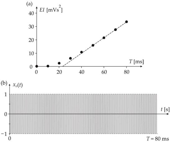
Figure 1. (a) Integral-square error $EI$ vs. time T; (b) signal $x_0\left(t\right)$ obtained for T = 80 ms.

Figure 1b shows the maximised signal $x_0\left(t\right)$, which has regular time-switchings. This should be considered a characteristic property of the integral-square criterion.

Figure 1a shows that in order to determine the error EI for any time greater than 0.05 ms, the coefficients $a_0$ and $a_1$ of the linear equation must be determined. The integral-square error $EI$ starts to increase linearly after the time at which the impulse response $k_{\mathrm{d}}$(t) achieves a value of zero. The nonlinear part of the characteristic $EI=f\left(T\right)$ is neglected in the analysis of the integral-square error, due to the short time T = (0–24 ms). If it is necessary to consider the upper bound of the dynamic error at a time $T$ of less than 24 ms, then a nonlinear approximation tool (such as polynomial regression) should be used.

Figure 2 shows the relationship between the signal $y_{\mathrm{d}}\left(t\right)$ defined by Equation (19) and the time $T.$

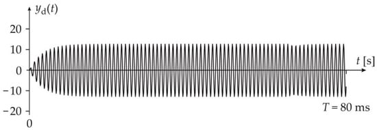
Figure 2. Relationship between the signal $y_{\mathrm{d}}\left(t\right)$ and the time $t$.

Based on the shape of the signal $y_{\mathrm{d}}\left(t\right)$, it can be concluded that in the initial moments, the magnitude of this signal increases in an oscillating manner and then reaches an approximately constant value. The regular and oscillatory shape of this error results from the regular switching of the signal $x_0\left(t\right)$ shown in Figure 1b.

Figure 3 shows the relationship between the error $EI \left(x_0\right)$ and the number of iterations $i$ of the iterative algorithm described by Equations (16)–(18). This relationship was determined for a time T = 80 ms, i.e., for the maximum time value included in Table 2.

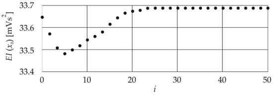
Figure 3. Relationship between the error $EI \left(x_0\right)$ and the number of iterations of the iterative algorithm.

Figure 3 shows that over approximately 25 iterations, the iterative algorithm converges, and the error $EI \left(x_0\right)$ is equal to 33.65 with an accuracy of two decimal places. Tests with other values of time $T$ confirmed that a maximum number of iterations of 50 was sufficient to achieve full convergence of the algorithm.

The discussion now turns to the relationship between the coefficients of the linear equation describing the error and two parameters of an accelerometer, i.e., the damping ratio and the time constant. The values of the coefficients $a_0$ and $a_1$ for constant values of both the voltage sensitivity $S_{\mathrm{V}}=1 \mathrm{V}/\left({\mathrm{ms}}^{-2}\right)$ and the non-damped natural frequency $f_0=1 \mathrm{kHz}$ are shown in Table 3.

Table 3. Matrix of values for coefficients $a_0$ and $a_1$.

$a_0$		$\tau$ [ms]
		0.100	0.350	0.600	0.850	1.10
$\beta$	0.01	−12.8	−37.5	−41.6	−43.6	−45.2
	0.02	−1.80	−4.90	−5.90	−5.90	−6.20
	0.03	−0.530	−1.30	−1.50	−3.30	−1.90
	0.04	−0.230	−0.650	−0.730	−0.740	−0.770
	0.05	−0.0500	−0.330	−0.320	−0.320	−0.310
$a_1$		$\tau$ [ms]
		0.100	0.350	0.600	0.850	1.10
$\beta$	0.01	0.580	1.69	1.90	1.97	2.02
	0.02	0.150	0.430	0.490	0.505	0.515
	0.03	0.0670	0.190	0.215	0.245	0.230
	0.04	0.0380	0.109	0.123	0.127	0.129
	0.05	0.0235	0.0700	0.0780	0.0805	0.0815

Figure 4 shows the relationship between the coefficient $a_0$ and: (a) the time constant for values of $S_{\mathrm{V}}=1 \mathrm{V}/\left({\mathrm{ms}}^{-2}\right),$ $f_0=1 \mathrm{kHz}$ and $\tau =0.10;$ and (b) the damping ratio for values of $S_{\mathrm{V}}=1 \mathrm{V}/\left({\mathrm{ms}}^{-2}\right),$ $f_0=1 \mathrm{kHz}$ and $\beta =0.010$.

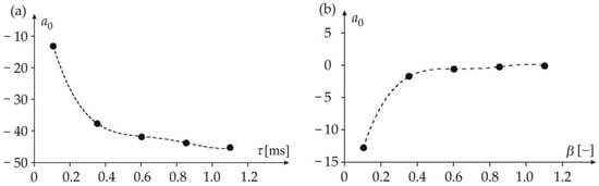
Figure 4. (a) Coefficient $a_0$ vs. $\tau$; (b) coefficient $a_0$ vs. $\beta$.

The regression functions corresponding to Figure 4 are

$$a_0\left(\tau \right)=10.2-28.3·\tau +587·{\tau }^2-583·{\tau }^3+179·{\tau }^4,$$

(24)

and

$$a_0\left(\beta \right)=-23.4+131·\beta -277·{\beta }^2+254·{\beta }^3-84.4·{\beta }^4,$$

(25)

while the regression accuracy values were obtained for the four-order polynomial and were $\mathsf{\Lambda }\left[a_0\left(\tau \right)\right]=2.86·{10}^{-3}$ and $\mathsf{\Lambda }\left[a_0\left(\beta \right)\right]=5.70·{10}^{-9},$ respectively. This is the polynomial structure that gives the highest value of the regression accuracy. Figure 4 shows that the function $a_0\left(\tau \right)$ decreases exponentially, but the function $a_0\left(\beta \right)$ increases exponentially.

Figure 5 shows a two-dimensional regression of the coefficient $a_1$, where the results were obtained by the same method as the regression in Figure 4.

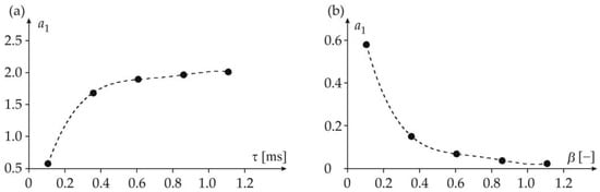
Figure 5. (a) Coefficient $a_1$ vs. $\tau$; (b) coefficient $a_1$ vs. $\beta$.

The regression functions corresponding to Figure 5 are

$$a_1\left(\tau \right)=-0.408+12.1·\tau -23.9·{\tau }^2+21.1·{\tau }^3-6.83·{\tau }^4,$$

(26)

and

$$a_1\left(\beta \right)=0.963-4.68·\beta +9.30·{\beta }^2-8.26·{\beta }^3+2.70·{\beta }^4,$$

(27)

while the regression accuracies were obtained from a fourth-order polynomial, and were $\mathsf{\Lambda }\left[a_1\left(\tau \right)\right]=1.25·{10}^{-9}$ and $\mathsf{\Lambda }\left[a_1\left(\beta \right)\right]=1.88·{10}^{-10},$ respectively. Figure 5 shows that the functions $a_1\left(\tau \right)$ and $a_1\left(\beta \right)$, respectively, increase and decrease exponentially. Figure 6a,b show the three-dimensional relationship between the coefficients $a_0$ and $a_1$ and the parameters $\tau$ and $\beta .$ These figures were created using the Curve Fitting toolbox built into the MATLAB software.

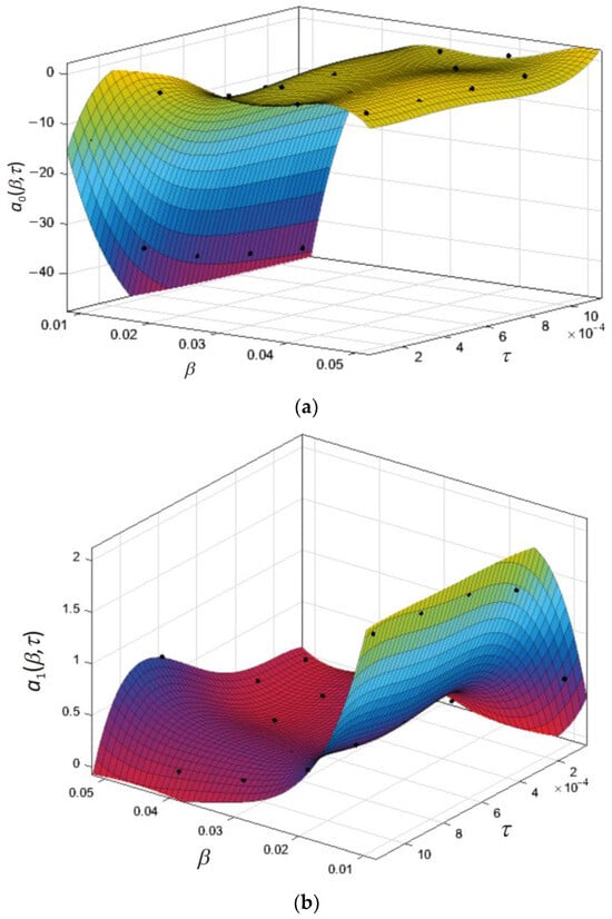
Figure 6. Three-dimensional relationship between the coefficients $a_0: \mathrm{subfigure} \left(a\right) \mathrm{and}$ $a_1:$ subfigure (b) and the parameters $\tau$ and $\beta$.

Figure 6 shows that the three-dimensional planes are stable functions in terms of variability, which significantly affects the value of the approximation accuracy of these planes and hence the value of the upper bound of the dynamic error obtained on this basis. The regression functions are fourth-order expressions, and in relation to the coefficients $a_0$ and $a_1$ are

$$\begin{gathered} a_0\left(\beta , \tau \right)=-65.5+1.16·{10}^4·\beta -3.00·{10}^5·\tau -6.21·{10}^5·{\beta }^2+1.52·{10}^7·\beta ·\tau \\ +3.54·{10}^8·{\tau }^2+1.34·{10}^7·{\beta }^3-2.77·{10}^8·{\beta }^2·\tau -9.33·{10}^9·\beta ·{\tau }^2 \\ -2.12·{10}^{11}·{\tau }^3-1.02·{10}^8·{\beta }^4+1.77·{10}^9·{\beta }^3·\tau +6.92·{10}^{10}·{\beta }^2·{\tau }^2 \\ +2.23·{10}^{12}·\beta ·{\tau }^3+5.14·{10}^{13}·{\tau }^4, \end{gathered}$$

(28)

and

$$\begin{gathered} a_1\left(\beta , \tau \right)=1.69-392·\beta +1.96·{10}^4·\tau +2.23·{10}^4·{\beta }^2-7.69·{10}^5·\beta ·\tau \\ -3.38·{10}^7·{\tau }^2-4.88·{10}^5·{\beta }^3+9.87·{10}^6·{\beta }^2·\tau +7.33·{10}^8·\beta ·{\tau }^2 \\ +2.73·{10}^{10}·{\tau }^3+3.70·{10}^6·{\beta }^4-3.66·{10}^7·{\beta }^3·\tau -3.99·{10}^9·{\beta }^2·{\tau }^2 \\ -2.53·{10}^{11}·\beta ·{\tau }^3-8.31·{10}^{12}·{\tau }^4 \end{gathered}$$

(29)

The corresponding accuracies are $\mathsf{\Lambda }\left[a_0\left(\beta , \tau \right)\right]=1.85$ and $\mathsf{\Lambda }\left[a_1\left(\beta , \tau \right)\right]=0.124,$ and the function that corresponds to the integral-square error is

$$EI\left(\beta ,\tau \right)=a_0\left(\beta , \tau \right)+a_1\left(\beta , \tau \right)·T,$$

(30)

which includes the functions defined by Equations (28) and (29).

Equation (30) allows for a quick and easy assessment of the accuracy of a charge-mode accelerometer, with the values of the parameters $\beta$ and $\tau$ taken from the ranges specified in Table 3 and constant values for the parameters $S_{\mathrm{V}}$ and $f_0$ of $1 \mathrm{V}/\left({\mathrm{ms}}^{-2}\right)$ and $1 \mathrm{kHz},$ respectively. Most importantly, this avoids the need to implement complex algorithms to determine the upper bound of the dynamic error. To determine this error, the parameters $\beta$ and $\tau$, which were obtained by parametric identification (practical experiment), should be substituted into Equations (28)–(30).

4. Conclusions

This paper presents a theoretical basis for and examples of regression for the maximum dynamic errors produced by charge-mode accelerometers. These theoretical solutions refer to the integral-square error denoted here by $EI\left(\beta ,\tau \right)$. Both the graphical and functional relationships between the error and selected parameters $\tau$ and $\beta$ of the considered accelerometer are determined. The results presented here relate to three-dimensional regression, whereas neural networks are used as criteria for the selection of the optimal regression order. For all of the examples presented in this paper, a fourth-order polynomial was obtained as the optimal choice, i.e., as generating the highest possible regression accuracy denoted by $\mathsf{\Lambda }\left[a_0\left(\beta , \tau \right)\right]$ and $\mathsf{\Lambda }\left[a_1\left(\beta , \tau \right)\right]$.

The solutions presented in this paper can be successfully applied for the needs of the multivariate regression. However, this requires the execution of a number of calculations of the error value, which is the product of the error number determined for particular parameters. In this way, it is possible to determine the error as the function of four parameters for a charge-mode accelerometer.

The functions that represent the regression are determined in such a way as to make it possible to calculate error values for any parameters of the mathematical model describing the selected accelerometer. This avoids the need to implement procedures for error determination.

The solutions presented in this paper can also be applied to other types of physical systems for which it is possible to determine a description by related mathematical models. However, this modelling should be implemented in accordance with the legal regulations applicable to these systems. The limitation of the proposed procedure is in the possibility of its practical application for the analysis of the charge-mode accelerometers with the parameters of the corresponding mathematical model included in the ranges for which the multivariate regression was determined. In such a case, it would be necessary to re-perform the research procedure discussed in the paper for the ranges covering both the accelerometer parameters and the uncertainties of the identification procedure related to these parameters.

References

- Morelle, C.; Théron, D.; Roch-Jeune, I.; Tilmant, P.; Okada, E.; Vaurette, F.; Grimbert, B.; Derluyn, J.; Degroote, S.; Germain, M.; et al. A micro-electro-mechanical accelerometer based on gallium nitride on silicon. Appl. Phys. Lett. 2023, 122, 033502. [Google Scholar] [CrossRef]
- Sanjuan, J.; Sinyukov, A.; Warrayat, M.F.; Guzman, F. Gyro-free inertial navigation systems based on linear opto-mechanical accelerometers. Sensors 2023, 23, 4093. [Google Scholar] [CrossRef]
- Goyal, D.; Pabla, B.S. Development of non-contact structural health monitoring system for machine tools. J. Appl. Res. Technol. 2016, 14, 245–258. [Google Scholar] [CrossRef]
- Wei, H.; Wu, M.; Cao, J. New matching method for accelerometers in gravity gradiometer. Sensors 2017, 17, 1710. [Google Scholar] [CrossRef] [PubMed]
- Shi, Y.; Jiang, S.; Liu, Y.; Wang, Y.; Qi, P. Design and optimization of a triangular shear piezoelectric acceleration sensor for microseismic monitoring. Geofluids 2022, 964502, 3964502. [Google Scholar] [CrossRef]
- Zhai, Z.; Xiong, X.; Ma, L.; Wang, Z.; Wang, K.; Wang, B.; Zhang, M.; Zou, X. A scale factor calibration method for MEMS resonant accelerometers based on virtual accelerations. Micromachines 2023, 14, 1408. [Google Scholar] [CrossRef]
- Juliani, F.; de Barros, E.; Mathias, M.H. A tool for controlling accelerometers. Secondary calibration data. Comptes Rendus Méc. 2013, 341, 687–696. [Google Scholar] [CrossRef]
- Scott, J.J.; Rowlands, A.V.; Cliff, D.P.; Morgan, P.J.; Plotnikoff, R.C.; Lubans, D.R. Comparability and feasibility of wrist- and hip-worn accelerometers in free-living adolescents. J. Sci. Med. Sport 2017, 2, 1101–1106. [Google Scholar] [CrossRef] [PubMed]
- Yu, H.; Zhang, X.; Shan, X.; Hu, L.; Zhang, X.; Hou, C.; Xie, T. A novel bird-shape broadband piezoelectric energy harvester for low frequency vibrations. Micromachines 2023, 14, 421. [Google Scholar] [CrossRef]
- Schilling, L.; Dalhoff, P. Piezoelectric patch transducers: Can alternative sensors enhance bearing failure prediction? J. Phys. Conf. Ser. 2019, 1356, 012015. [Google Scholar] [CrossRef]
- JCGM 100:2008; BIPM, IEC, IFCC, ILAC, ISO, IUPAC, IUPAP, and OIML, Guide to the Expression of Uncertainty in Measurement. JCGM: Sèvres, France, 1995.
- Bertuletti, S.; Cereatti, A.; Comotti, D.; Caldara, M.; Croce, U.D. Static and dynamic accuracy of an innovative miniaturized wearable platform for short range distance measurements for human movement applications. Sensors 2017, 17, 1492. [Google Scholar] [CrossRef]
- Layer, E. Modelling of Simplified Dynamical Systems; Springer: Berlin/Heidelberg, Germany; New York, NY, USA, 2002; ISBN 9783642628566. [Google Scholar]
- Rutland, N.K. The principle of matching: Practical conditions for systems with inputs restricted in magnitude and rate of change. IEEE Trans. Autom. Control 1994, 39, 550–553. [Google Scholar] [CrossRef]
- Layer, E.; Tomczyk, K. Measurements: Modelling and Simulation of Dynamic Systems; Springer: Berlin/Heidelberg, Germany, 2010; ISBN 3642045871/9783642045875. [Google Scholar]
- Yu, J.C.; Lan, C.B. System modeling of microaccelerometer using piezoelectric thin films. Sens. Actuator A Phys. 2001, 88, 178–186. [Google Scholar] [CrossRef]
- Sun, X.T.; Jing, X.J.; Xu, J.; Cheng, L. A quasi-zero-stiffness-based sensor system in vibration measurement. IEEE Trans. Ind. Electron. 2014, 61, 5606–6114. [Google Scholar] [CrossRef]
- Link, A.; Täbner, A.; Wabinski, W.; Bruns, T.; Elster, C. Modelling accelerometers for transient signals using calibration measurement upon sinusoidal excitation. Measurement 2007, 40, 928–935. [Google Scholar] [CrossRef]
- JCGM 101:2008; BIPM, IEC, IFCC, ILAC, ISO, IUPAC, IUPAP, and OIML. Evaluation of Measurement Data: Supplement 1 to the Guide to the Expression of Uncertainty in Measurement—Propagation of Distributions Using a Monte Carlo Method. JCGM: Sèvres, France, 2008.
- Tomczyk, K. Impact of uncertainties in accelerometer modeling on the maximum values of absolute dynamic error. Measurement 2016, 80, 71–78. [Google Scholar] [CrossRef]
- Honig, M.L.; Steiglitz, K. Maximizing the output energy of a linear channel with a time and amplitude limited input. IEEE Trans. Inf. Theory 1992, 38, 1041–1052. [Google Scholar] [CrossRef][Green Version]
- Elia, M.; Taricco, G.; Viterbo, E. Optimal energy transfer in bandlimited communication channels. IEEE Trans. Inf. Theory 1999, 45, 2020–2029. [Google Scholar] [CrossRef][Green Version]
- Gu, S.; Luo, Z.; Chu, Y.; Xu, Y.; Jiang, Y.; Guo, J. Trace Alignment Preprocessing in Side-Channel Analysis Using the Adaptive Filter. IEEE Trans. Inf. Forensics Secur. 2023, 18, 5580–5591. [Google Scholar] [CrossRef]
- Guo, J.; Liu, Y.; Lin, L.; Li, S.; Cai, J.; Chen, J.; Huang, W.; Lin, Y.; Xu, J. Chromatic Plasmonic Polarizer-Based Synapse for All-Optical Convolutional Neural Network. Nano Lett. 2023, 23, 9651–9656. [Google Scholar] [CrossRef]
- Krebs, R.; Rothstein, B.; Roelle, J. Rubrics Enhance Accuracy and Reduce Cognitive Load in Self-Assessment. Metacogn. Learn. 2022, 17, 627–650. [Google Scholar] [CrossRef]
- Peiyuan, Z.; Guorui, X.; Lan, D. Initial performance assessment of Galileo High Accuracy Service with software-defined receiver. GPS Solut. 2023, 28, 2. [Google Scholar] [CrossRef]
- Egert, J.; Kreutz, C. Rcall: An R interface for MATLAB. SoftwareX 2023, 21, 101276. [Google Scholar] [CrossRef]
- Roman, C.; Morales, M.G. On the integration of Mathcad capabilities into a mass transfer operations course in chemical engineering studies. Comput. Appl. Eng. Educ. 2022, 31, 938–951. [Google Scholar] [CrossRef]
- Tomczyk, K. Assessment of convergence of the algorithm for determining the upper bound of dynamic error on the example of acceleration sensors. In Proceedings of the 20th International Conference on Research and Education in Mechatronics (REM), Wels, Austria, 23–24 May 2019; pp. 1–6. [Google Scholar] [CrossRef]
- Sinha, P. Multivariate polynomial regression in data mining: Methodology, problems and solutions. Int. J. Sci. Eng. Res. 2013, 4, 962–965. [Google Scholar]
- Rady, E.-H.A.; Ziedan, D. Estimation of population total using local polynomial regression with two auxiliary variables. J. Stat. Appl. Probab. 2014, 2, 129–136. [Google Scholar] [CrossRef]
- Tomczyk, K. Polynomial approximation of the maximum dynamic error generated by measurement systems. Prz. Elektrotechniczny 2019, 95, 124–127. [Google Scholar] [CrossRef]
- Pintelon, R.; Schoukens, J. System Identification: A Frequency Domain Approach; John Wiley & Sons: Hoboken, NJ, USA, 2012. [Google Scholar] [CrossRef]
- Bargues, À.S.; Sanz, J.-L.P.; Martín, R.M. Optimal experimental design for parametric identification of the electrical behaviour of bioelectrodes and biological tissues. Mathematics 2022, 10, 837. [Google Scholar] [CrossRef]
- Tomczyk, K. Problems in modelling charge output accelerometers. Metrol. Meas. Syst. 2016, 23, 645–659. [Google Scholar] [CrossRef]
Disclaimer/Publisher’s Note: The statements, opinions and data contained in all publications are solely those of the individual author(s) and contributor(s) and not of MDPI and/or the editor(s). MDPI and/or the editor(s) disclaim responsibility for any injury to people or property resulting from any ideas, methods, instructions or products referred to in the content. |
© 2023 by the authors. Licensee MDPI, Basel, Switzerland. This article is an open access article distributed under the terms and conditions of the Creative Commons Attribution (CC BY) license (https://creativecommons.org/licenses/by/4.0/).