GAN-Based Abrupt Weather Data Augmentation for Wind Turbine Power Day-Ahead Predictions

Abstract

This study introduces a data augmentation technique based on generative adversarial networks (GANs) to improve the accuracy of day-ahead wind power predictions. To address the peculiarities of abrupt weather data, we propose a novel method for detecting mutation rates (MR) and local mutation rates (LMR). By analyzing historical data, we curated datasets that met specific mutation rate criteria. These transformed wind speed datasets were used as training instances, and using GAN-based methodologies, we generated a series of augmented training sets. The enriched dataset was then used to train the wind power prediction model, and the resulting prediction results were meticulously evaluated. Our empirical findings clearly demonstrate a significant improvement in the accuracy of day-ahead wind power prediction due to the proposed data augmentation approach. A comparative analysis with traditional methods showed an approximate 5% increase in monthly average prediction accuracy. This highlights the potential of leveraging mutated wind speed data and GAN-based techniques for data augmentation, leading to improved accuracy and reliability in wind power predictions. In conclusion, this paper presents a robust data augmentation method for wind power prediction, contributing to the potential enhancement of day-ahead prediction accuracy. Future research could explore additional mutation rate detection methods and strategies to further enhance GAN models, thereby amplifying the effectiveness of wind power prediction.

1. Introduction

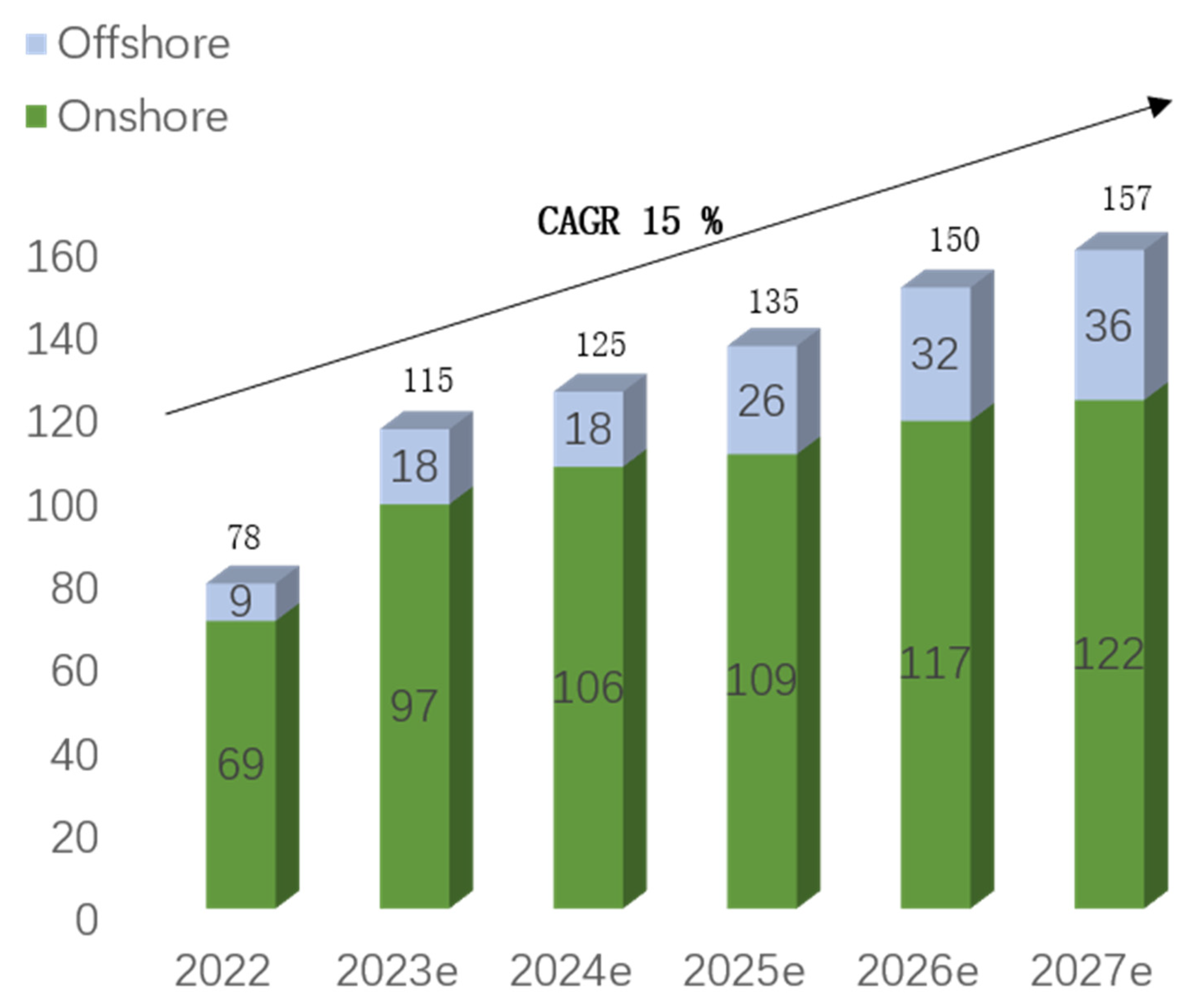
According to the International Energy Agency (IEA) 2023 Electricity Market Report, the global installed capacity of wind power reached 906 GW by the end of 2022, accounting for approximately 8% of the total global energy production. It is expected to exceed 1 TW for the first time this year [1]. Figure 1 illustrates the forecast by the Global Wind Energy Council (GWEC) for new wind turbine installations from 2022 to 2026, indicating an expected annual compound growth rate of 15%. The IEA aims for renewable energy to contribute 61% of total electricity generation by 2030, and wind power, representing around 20% of renewable energy, has emerged as one of the most effective decarbonization tools for the power system [2]. However, due to the volatility of wind power generation, integrating a large amount of wind energy into the power grid poses significant challenges to the safety and economic operation of the power system. Therefore, accurate power prediction results serve as the foundation for power system analysis and operational control.

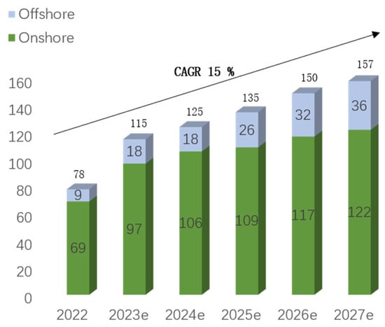
Figure 1. The outlook for new installations from 2022 to 2027 (unit: GW).

Short-term forecast results can be utilized for decision-making and operational purposes in fields such as computer science and meteorology. These include activities such as formulating power dispatch plans, optimizing generation resource scheduling, responding to emergencies, and conducting market transactions. Stakeholders, such as power market participants, energy traders, and power plant operators, rely on short-term forecast data for their business activities and decision-making processes. The term “recent power forecast” refers to the short-term forecast for the upcoming hours, up to a day. In China, renewable energy plants are required to provide a forecast of their power generation for every 15-min interval for the next 0–24 h to the grid company before 8:00 AM [3].

Currently, there exist three main categories of wind power prediction methods: physical models, statistical models, and artificial intelligence models [4]. Physical models often depend on numerical weather prediction (NWP) or time series models. They incorporate various relevant variables to predict wind speeds or wind power [5]. However, these physical models have limitations in achieving accurate short-term wind power forecasts due to their high computational complexity and slow updates. Traditional statistical models, such as autoregressive moving average (ARMA) models [6] and autoregressive integrated moving average (ARIMA) models [7], are commonly used for short-term forecasts within 6 h. These models assist in the control and tracking of wind turbines [8,9]. However, most statistical models assume linearity and struggle to handle the irregular and nonlinear characteristics of wind power series.

In recent years, several artificial intelligence models have successfully improved wind power prediction by capturing complex, nonlinear relationships within historical data [10,11]. The following deep learning models have been developed and utilized over the past six years: convolutional neural networks (CNN) [12], recurrent neural networks (RNN), long short-term memory (LSTM) [13], deep residual networks [14], stacked autoencoders, deep neural networks (DNN) [15], gated recurrent networks [16], and deep hybrid models [17]. Previous research has demonstrated that deep learning-based models outperform statistical and physical models [18]. Compared with other renewable energy sources, wind power prediction models based on deep neural networks not only enhance forecast accuracy but also reduce operational costs, thus increasing the competitiveness of wind energy. Recent studies have proposed various approaches to wind power prediction. Some have relied on lagged wind power data or directly correlated variables, such as wind speed and its periodicity, to calculate wind power using specific power curves. For instance, Xu Peihua et al. [19] introduced the DWT_AE_BiLSTM model based on deep learning for short-term wind power prediction, achieving an accuracy improvement of over 3.4% compared with traditional algorithms. Bangru Xiong et al. [20] suggested that the AMC-LSTM hybrid model, which integrates multiscale extended features and dynamically allocates weights to physical attribute data using attention mechanisms, effectively addresses the issue of differentiating the importance of input data. Sahra Khazaei et al. [21] proposed a high-precision hybrid method for short-term wind power prediction utilizing historical wind farm data and numerical weather prediction (NWP) data, where the accuracy of the forecast was significantly impacted by the feature selection method. Ling Huang et al. [22] presented the BiLSTM-CNN-WGAN-GP model for short-term wind power prediction, which applied a generative adversarial network (WGAN-GP) to extract data distribution characteristics for wind power output and improve prediction accuracy.

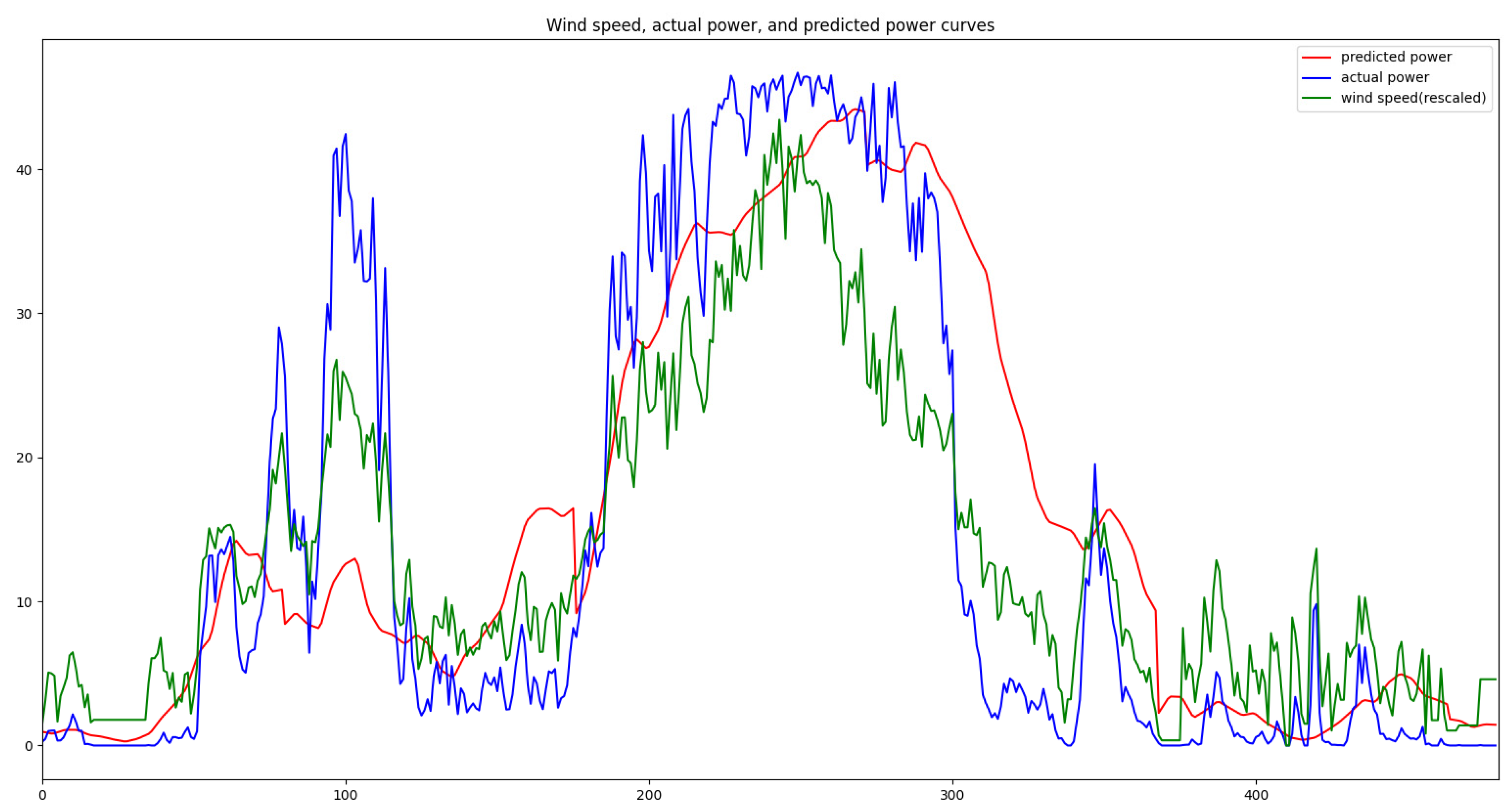
Although artificial intelligence models have achieved significant effectiveness in wind power prediction, the characteristics of wind power, such as volatility, periodicity, time-shift, and aggregation [23], result in varying forecast accuracies for the same model in different seasons. Taking a wind farm in Zaoyang, Hubei Province, China as an example, the forecast accuracy is generally higher in the summer and autumn compared with spring and winter (refer to Table 1). By analyzing historical data, it can be observed that inaccurate forecasts often occur during weather transitions (sudden weather changes) where the data tends to be underestimated. In China, the east wind prevails in the spring, the southeast wind prevails in the summer, the west wind prevails in autumn, and the northwest wind prevails in the winter. The east and northwest winds exhibit drastic changes and are often accompanied by occurrences of ice cover, whereas the southeast and west winds are relatively calm (refer to Figure 2). Addressing forecast accuracy during weather transitions could effectively improve overall forecast accuracy for this wind farm.

Table 1. Monthly wind power prediction accuracy statistics for a wind farm in 2022.

Season	Month	LSTM	AMC-LSTM	DWT_AE_BiLSTM	AE_BiLSTM	Accuracy
Spring	3	71.23	70.54	67.41	66.85	72.06
	4	65.88	74.26	70.77	70.15
	5	78.44	76.72	76.56	75.85
Summer	6	74.35	81.13	82.13	81.35	79.37
	7	83.73	83.34	88.53	86.93
	8	73.22	77.02	70.59	70.1
Autumn	9	85.18	84.69	84.13	83.25	79.43
	10	81.02	81.99	72.25	71.61
	11	80.51	80.55	74.33	73.67
Winter	12	77.91	75.58	71.79	71.46	74.60
	1	74.70	74.29	62.69	63.56
	2	82.73	80.72	80.19	79.5

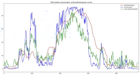
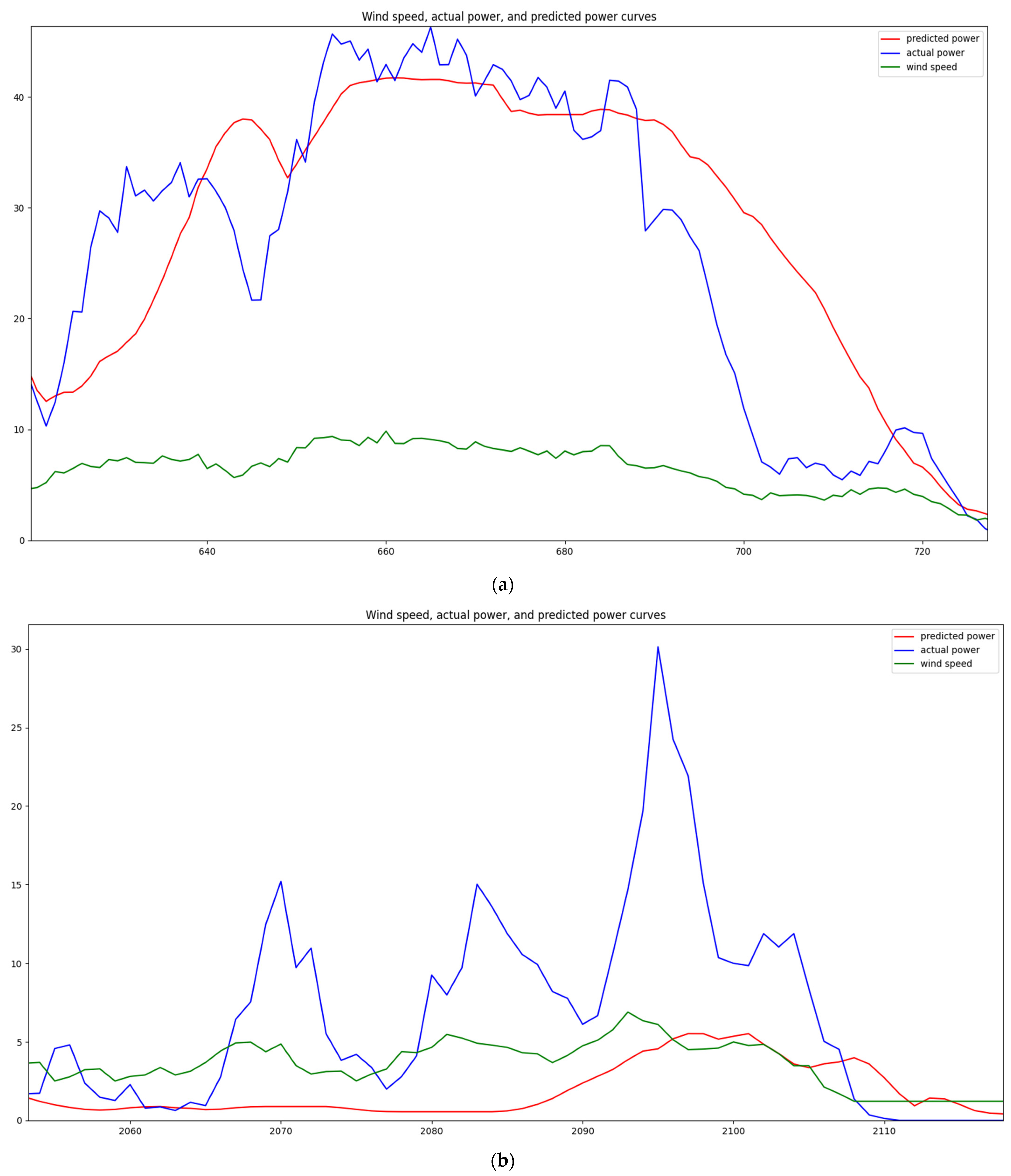
Figure 2. Wind speed, actual power, and predicted power curves at a wind farm.

The authors suggest that the underestimation of forecast data during weather transitions is caused by insufficient samples of weather transition data, resulting in inadequate training of the model. In this study, two volatility indicators, namely mutation rate (MR) and local mutation rate (LMR), are introduced. These indicators, distinct from the volatility characteristic indicators mentioned in [24], such as amplitude rate (AR), fluctuation rate (FR), and ramp rate (RR), effectively detect weather transition data. Moreover, a data training model similar to TimeGAN [25] is used to generate weather data samples that exhibit the characteristics of weather transitions. To ensure the usability of the sample data for training, a wind/power function generation algorithm was proposed. The generated training samples, combined with samples generated from historical data, were used to train the wind power prediction model. The results demonstrated a significant improvement in forecast accuracy for the same model, with the most pronounced increase observed during the winter and spring seasons, thus confirming the effectiveness of this model framework.

The remaining sections of this paper are organized as follows: Section 2 presents the relevant content of the proposed method. In Section 3, the implementation framework of the method, as well as the extraction of meteorological data during weather transitions and the generation of training samples, are described in detail. Section 4 provides a detailed analysis of the prediction results of the algorithm for selected stations. Finally, Section 5 summarizes the algorithm.

2. Related Work

2.1. Wind Speed Fluctuation and Variability Metrics

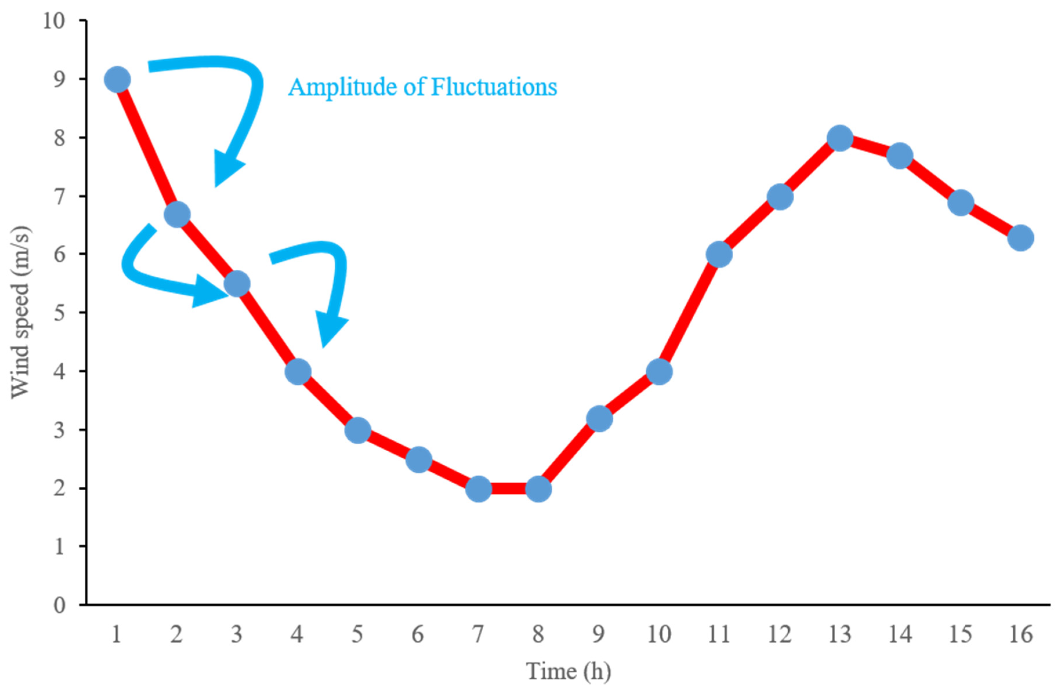
The fluctuation of wind speed is a key characteristic of wind energy. In the literature [24], a change in wind speed between adjacent time points in a continuous time series is defined as a fluctuation, as illustrated in Figure 3. The magnitude of the fluctuation, or fluctuation amplitude (FA), quantifies the degree of variation in wind speed or power between adjacent time points. It is typically computed as the average within a time interval. Smaller values indicate lower fluctuation and better stability. While fluctuation amplitude focuses on absolute variation, the fluctuation rate (FR) considers the relative variation. Formulas (2) and (3) represent the calculations for fluctuation amplitude and fluctuation rate. Fluctuation amplitude and fluctuation rate focus on the instantaneous changes within adjacent time windows.

$${\gamma }_i={\vartheta }_{i+1}-{\vartheta }_i$$

(1)

$$FA=\frac{1}{n-1}{\sum }_{i=1}^{n-1}\left|{\gamma }_i\right|$$

(2)

$$FR=\frac{1}{n-1}{\sum }_{i=1}^{n-1}|\frac{{\gamma }_i}{{\vartheta }_i}|$$

(3)

Figure 3. Wind speed fluctuation diagram.

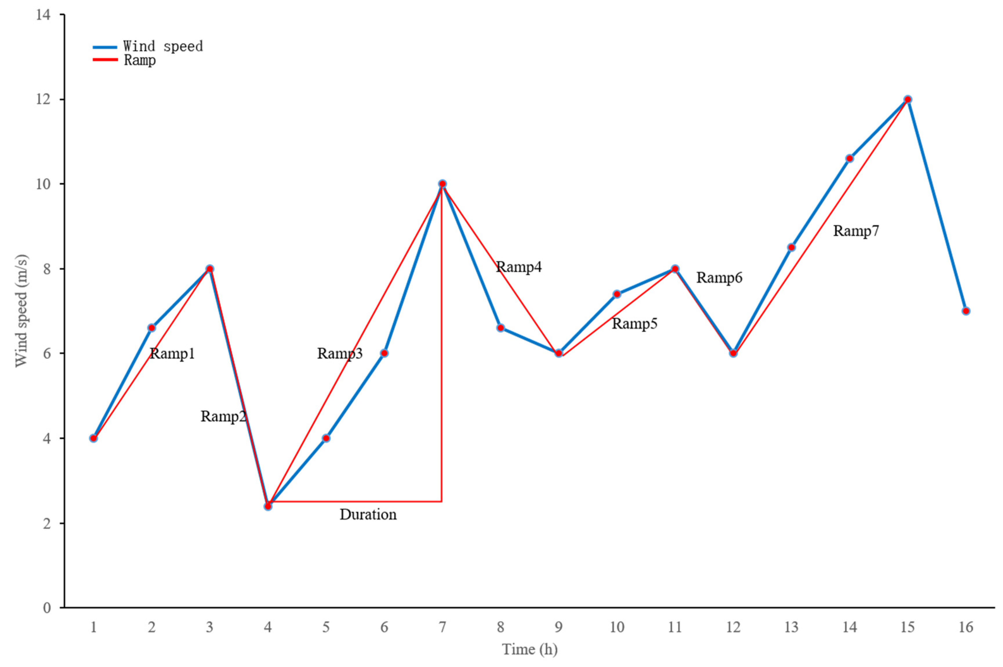
However, wind speed or power may experience continuous upward or downward trends over a period of time, and these large variations pose challenges to the power system. Therefore, the ramp rate (RR) metric is introduced to quantify the monotonic changes within continuous time windows. Renewable energy sources, such as wind and solar, often exhibit ramp events, which are sudden increases or decreases in power generation. Currently, there is no standardized definition for ramp events in the industry. In reference [26], a ramp event is defined as the process from one extreme value to the next, where these extreme points are not adjacent in time. As shown in Figure 4, the red line represents a ramp event, describing a continuous increase or decrease in a certain physical quantity over a period of time. The length of this process is not limited; as long as it belongs to the same upward or downward trend, it is considered a ramp event. Thus, fluctuation rate and ramp rate complement each other, providing a comprehensive and detailed characterization of the fluctuations in wind speed time series.

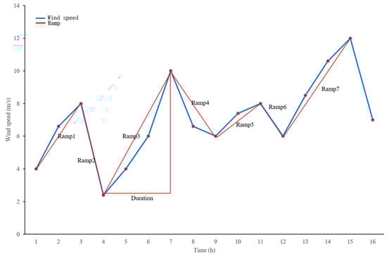
Figure 4. Illustration of a ramping event.

Ramp rate of a specific ramping event:

$${\rho }_m=\frac{{\vartheta }_j-{\vartheta }_i}{t_j-t_i}$$

(4)

Ramp rate over a period of time:

$$N={\sum }_{i=1}^{n}R\left(i,j\right)$$

(5)

Average ramp rate over a period of time:

$$RR=\frac{1}{N}\sum |{\rho }_m|$$

(6)

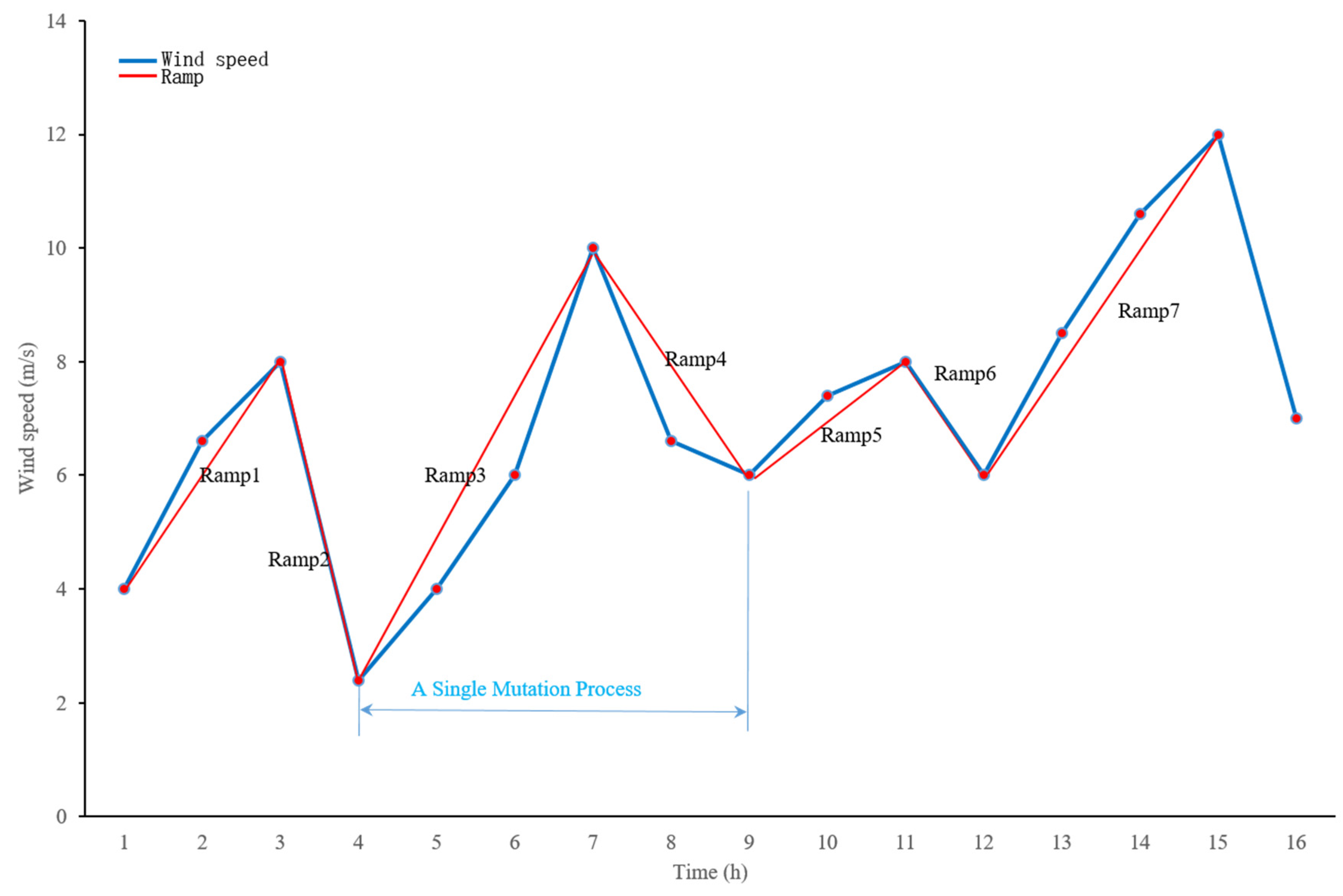
Although the combination of ramp rate and fluctuation rate can describe most wind speed fluctuations, it is not suitable for describing weather transitions. For example, Figure 5 depicts two scenarios, A and B. Conventional deep learning models can accurately predict the wind speed fluctuations in Scenario A (Figure 5a). However, the predictions are generally inaccurate for Scenario B (Figure 5b). To distinguish between these two types of wind speed fluctuations, we propose a new wind speed feature metric called the mutation rate (MR). Unlike the ramp rate, which separately considers upward and downward ramps, the mutation rate considers each upward and downward ramp (excluding the beginning and the end) as one mutation. Each mutation represents a local transition, as illustrated in Figure 6. The calculation formula for the local mutation rate (LMR) is as follows:

$$\mathrm{LMR}=\frac{\left|v_{top}-v_1\right|}{t_1}+\frac{\left|v_{top}-v_2\right|}{t_2}$$

(7)

where $v_{top}$ represents the vertex of the mutation, $v_1$ and $v_2$ respectively represent the bottom points of the upward and downward ramps, and $t_1$ and $t_2$ represent the time span of each ramp. The average of all local mutations is referred to as the mutation rate (MR). The specific formula is as follows:

$$\mathrm{MR}=\frac{1}{n}{\displaystyle \sum _{i=1}^n\frac{\left|v_{topi}-v_{i1}\right|}{t_{i1}}+\frac{\left|v_{topi}-v_{i2}\right|}{t_{i2}}}$$

(8)

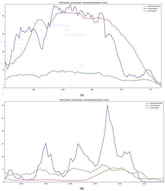
Figure 5. Prediction performance under different mutation rates: (a) low mutation rate curves; (b) high mutation rate curves.

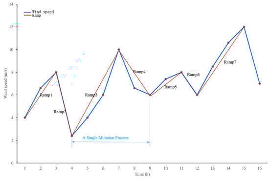
Figure 6. A single mutation process.

It should be noted that each local mutation is initiated by an upward ramp and terminated by a downward ramp. If a wind speed time series begins with a downward trend or ends with an upward ramp, they must be evaluated separately. The combination of fluctuation rate, ramp rate, and mutation rate provides a comprehensive characterization of both overall fluctuations and the magnitude of local fluctuations in a wind speed sequence.

A high ramp rate in wind speed does not necessarily imply a high mutation rate in the context of computer and power prediction. For example, situations with low fluctuations, even with a high ramp rate, would not result in significant changes in the magnitude of the mutation rate. In such cases, wind speed transitions are typically smooth, and most conventional algorithms can accurately predict power output. On the other hand, when both ramp rate and volatility are high, it inevitably leads to a high mutation rate, which typically results in larger errors for typical power prediction algorithms. Table 2 provides a detailed illustration of the relationship between these three metrics and the accuracy of power prediction.

Table 2. Relationship between metrics and the accuracy of power prediction.

No.	FR	RR	MR	Weather	Accuracy
1	High	High	High	Strong convective weather in summer	Low
2	High	Low	Medium	Rainy weather in spring and autumn	Medium
3	Low	High	High	Dusty and cooler weather	Low
4	Low	Low	Low	Sunny and fine weather	High

2.2. TimeGAN Model

TimeGAN (time-series generative adversarial network) is a model proposed by Jinsung Yoon et al. from the University of California at NeurIPS 2019 [25], designed for generating time-series data. The main idea is to combine the versatility of unsupervised GAN methods with the conditional probability principles provided by supervised auto-regressive models to generate time-series data that preserves temporal dynamics. TimeGAN consists of four main components: an embedding function, recovery function, sequence generator, and sequence discriminator. The first two components form an autoencoder, whereas the latter two are part of the GAN framework [27]. As a result, TimeGAN is capable of learning embedded features, generating representations, and iterating over time. The embedding network provides a latent space where the adversarial network operates, synchronizing the latent dynamics of real and synthetic data through supervised loss. The structure is illustrated in Figure 7.

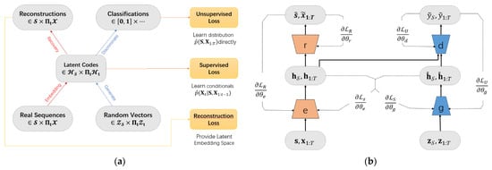
Figure 7. Structural diagrams of TimeGAN: (a) a block diagram and (b) training scheme.

2.3. Wind Speed–Power Curve

According to the definition of the IEC 61400-12-1 [28] standard, the wind speed–power curve of a wind turbine refers to the relationship between the turbine’s output power and the 15-min average wind speed. If other factors are not considered (neglecting the internal characteristics of the wind turbine), the input wind speed significantly influences a turbine’s output power (i.e., active power).

$$P=f(\mathrm{V})$$

(9)

Here, P represents the active power output of the wind turbine in kW, and V is the measured wind speed in m/s.

For each type of wind turbine model, manufacturers establish a theoretical wind speed–power curve. By comparing the actual wind speed–power curve with the theoretical one, it is possible to determine whether the wind turbine is operating in an overload, underload, or normal load state. However, due to significant differences between the actual operational environment of wind turbines and their ideal design conditions, the theoretical wind speed–power curve may deviate in real wind farm settings. Consequently, to accurately depict the operational state of wind turbines, it becomes necessary to construct wind farm-specific actual wind speed–power curves.

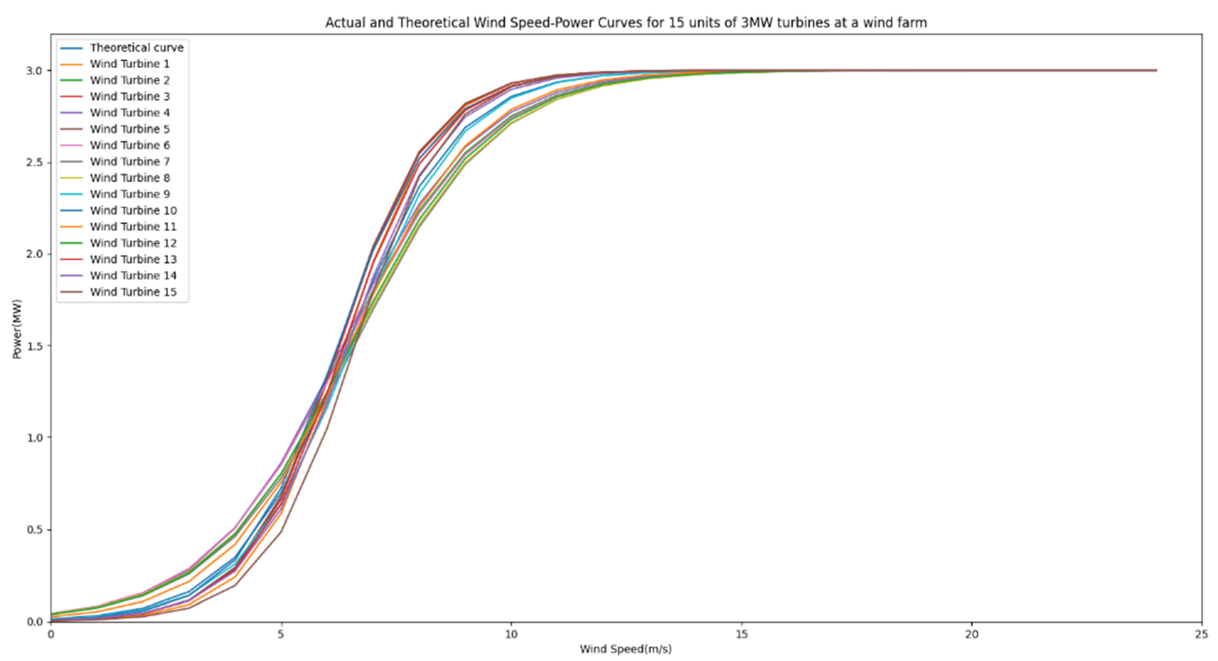
Figure 8 illustrates the scatter plot of actual wind speed–power data points and the theoretical wind speed–power curve for a 3 MW turbine model consisting of 15 units at a domestic wind farm. It is evident from the graph that certain discrepancies exist between the actual wind speed–power data points and the theoretical curve.

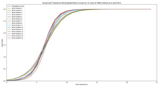
Figure 8. Actual and theoretical wind speed–power curves for 15 units of turbines.

During the design phase of wind turbines, the wind speed–power curve theoretically defines the power characteristics and operational traits of the wind turbine. It also enables a theoretical assessment of energy generation and efficiency, thus measuring the wind turbine’s capability to convert wind energy. Hence, the wind speed–power curve serves as a vital technical assessment criterion for wind farm site selection and is a significant indicator of unit performance. The theoretical design of the wind speed–power curve constitutes an integral aspect of overall wind turbine design.

The wind speed–power curve not only facilitates the evaluation of a wind turbine’s energy generation performance but also plays a substantial role in practical applications:

(1)

Cleaning of operational data: Numerous anomalies occur during wind turbine operation, such as unscheduled shutdowns, malfunctioning wind speed measurement sensors, curtailment, unit disconnection, blade damage, etc., leading to abnormal data. Data cleaning can be performed based on the wind speed–power curve. For example, the anomalies at points numbered 1, 2, and 3 in Figure 9 need to be addressed.

(2)

Fault diagnosis: Anomalies evident in wind speed–power scatter points often signify specific faults or anomalies in the unit. For instance, in Figure 9, anomalies at points 1 and 4 represent instances where wind speed meets the generation requirement, but the unit fails to generate power. Conversely, when wind speed does not meet the generation requirement, but produces power (as seen at point 2), potential causes could involve malfunctions of the unit, acquisition equipment, or communication equipment. Point 3 indicates a scenario where wind speed meets the generation requirement, yet the unit’s output is low; combining this information with temperature readings can help determine whether this is due to blade icing.

(3)

Overgeneration and undergeneration: By comparing the actual wind speed–power curve with its theoretical counterpart, it is possible to assess overgeneration or undergeneration states when exceeding the rated wind speed. If the actual power output surpasses the theoretical rated power, the unit is in an overgeneration state. Conversely, if the actual power output is lower than the theoretical rated power, the unit is in an undergeneration state.

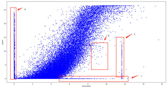
Figure 9. Scatter plot of wind speed–power for wind farm units.

Figure 9. Scatter plot of wind speed–power for wind farm units.

3. Day-Ahead Prediction Algorithm Processing Framework

3.1. Introduction of the Framework

To address the demand for day-ahead prediction, we propose an algorithmic processing framework that meets application requirements. The steps are as follows:

(1)

Construct a training set input X, containing actual wind speed sequences, and a training output Y of an actual power sequence. The training set may also include actual wind direction, numerical forecast data sequences (wind speed and wind direction), as well as time sequences (year, month, day, hour, and minute).

(2)

Utilize a sigmoid approximation algorithm to eliminate training data that do not adhere to the wind speed–power curve.

(3)

Calculate the mutation rate for each data group using the mutation rate formula (Equations (7) and (8)). Extract a portion of training data with the highest mutation rates based on the proportion α to form a new training dataset.

(4)

Employ the newly created training dataset as input to train the data augmentation model.

(5)

Utilize the trained data augmentation model to generate new training data.

(6)

Use the sigmoid approximation algorithm to remove generated training data that does not conform to the wind speed–power curve.

(7)

Merge the newly generated dataset with the originally constructed initial dataset and shuffle the dataset according to specified rules.

(8)

Train the data using the designed power prediction model.

(9)

Predict power and perform error analysis on the prediction results.

The algorithm processing framework is depicted in Figure 10.

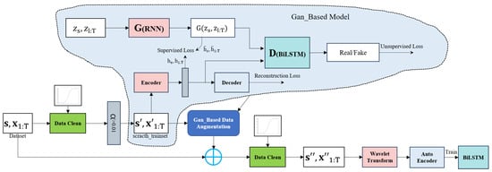
Figure 10. Day-ahead predict algorithm processing framework.

3.2. Data-Cleaning Methods

Due to factors such as communication interruptions and equipment malfunctions, certain data points may deviate from the average wind power curve. For instance, there are instances of higher power output at lower wind speeds. This discrepancy may be attributed to faults in the wind speed measurement apparatus. Conversely, during periods of elevated wind speeds, a significant reduction in power output could be indicative of equipment shutdowns.

Consequently, the raw data collected by the system must undergo a specific process of cleaning and interpolation before it can be utilized further. The wind power curve is approximated using the sigmoid function (Equation (10)) for solution. The parameters to be solved are a and b, where a represents the slope and b represents the center point.

$$f_{sigmod}=\frac{1.0\times C_{capacity}}{1.0+e^{-a\times x+a\times b}}$$

(10)

Once the wind power curve function is obtained, it can be processed with specific thresholds for delineation. This process will result in the creation of two enveloping curves centered around the fitted wind power curve. Data beyond the envelope curves will be flagged and subjected to cleaning procedures, whereas data within the envelope boundaries will be retained.

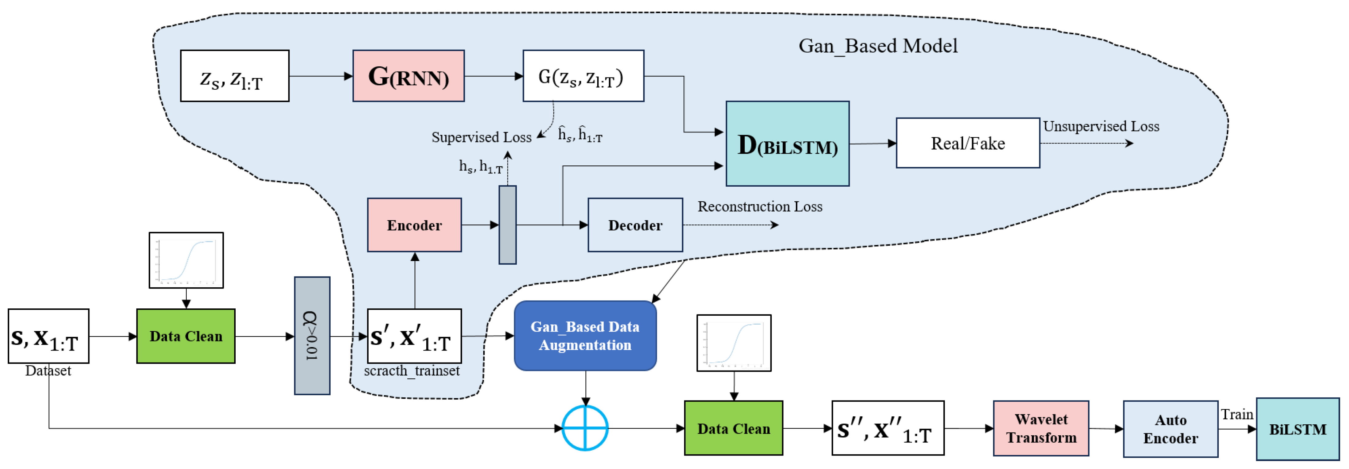
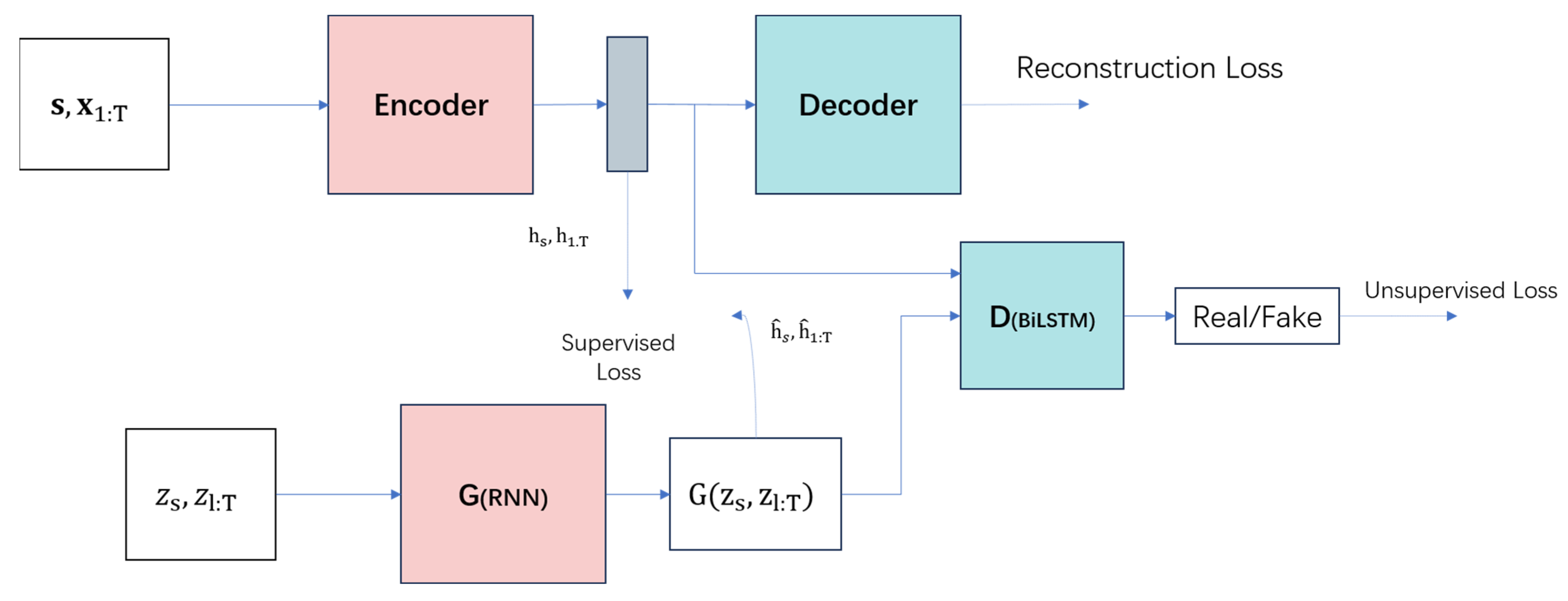
3.3. Data Augmentation Model based on GAN

Data augmentation presents a framework (Figure 11) that leverages both traditional unsupervised GAN training methods and controllable supervised learning techniques. By combining an unsupervised GAN network with a supervised autoregressive model, the network aims to generate a time series with preserved temporal dynamics. The architecture is illustrated in Figure 11. The framework’s input is perceived to consist of two elements: a static feature and temporal feature. S represents the static feature vector at the encoder input, whereas X represents the temporal feature vector. The generator takes tuples of static and temporal random feature vectors extracted from known distributions. Real and synthetic latent codes $h$ and $\widehat{h}$ are used to compute the network’s supervised loss. The discriminator receives tuples of real and synthetic latent codes, classifying them as real ($y$) or synthetic ($\tilde{y}$).

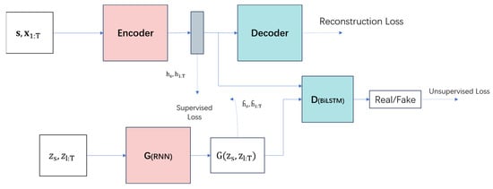
Figure 11. GAN-based data augmentation framework.

3.3.1. Embedded and Recovery Functions

Within the data augmentation model, an embedding function (Equation (11)) is employed to transform original time series data into a lower-dimensional embedding representation, capturing essential data features. The recovery function (Equation (12)) then transforms the embedding representation back into the original form of time series, preserving the temporal dynamics of the data. In these equations, the tilde (~) operator denotes the representation as real or synthetic. These two components together constitute part of the autoencoder, learning the latent representation of time-series data through an encoding and decoding process, laying the foundation for the generation process. The embedding and recovery functions can be parameterized using any chosen architecture, with the requirement that they are autoregressive and adhere to a causal order (i.e., the output at each step depends only on preceding information).

$$\mathrm{embedded} \mathrm{function}: \begin{array}{l}{\mathrm{h}}_S=e_S(\mathrm{S})\\ {\mathrm{h}}_t=({\mathrm{h}}_S,{\mathrm{h}}_{t-1},{\mathrm{x}}_t)\end{array}$$

(11)

$$\mathrm{recovery} \mathrm{function}: \begin{array}{l}\tilde{\mathrm{S}}=r_S({\mathrm{h}}_S)\\ {\tilde{\mathrm{X}}}_t=r_x({\mathrm{h}}_t)\end{array}$$

(12)

3.3.2. Generator and Discriminator Functions

In the data augmentation model, the generator (Equation (13)) employs the embedding function and random noise input to produce new synthetic time-series data. Through training, the generator becomes capable of preserving temporal continuity and naturalness. The discriminator function (Equation (14)) assesses the similarity between generated and real sequences, gradually aligning the generated data’s distribution with that of real data through adversarial training mechanisms.

$$\mathrm{generator}: \begin{array}{l}{\widehat{\mathrm{h}}}_S=g_S({\mathrm{Z}}_{\mathrm{S}})\\ {\widehat{\mathrm{h}}}_t=g_{\chi }({\widehat{\mathrm{h}}}_S,{\widehat{\mathrm{h}}}_{t-1},{\mathrm{z}}_t)\end{array}$$

(13)

$$\mathrm{Discriminator}: \begin{array}{l}{\tilde{y}}_S=d_S({ \tilde{\mathrm{h}}}_S)\\ {\tilde{y}}_t=d_{\chi }({ \overleftarrow{\mathrm{u}}}_t,{ \overrightarrow{\mathrm{u}}}_t)\end{array}$$

(14)

3.3.3. Joint Learning of Encoding, Generation, and Iteration

The data augmentation model employs multiple loss functions for training, including the reconstruction loss of the embedding function (Equation (15)), adversarial losses of the generator and discriminator (Equation (16)), as well as temporal coherence loss (Equation (17)). By optimizing these loss functions, the model can learn the temporal dynamics and features of time-series data. The training process of the model follows an iterative approach, where optimization functions are used to update model parameters in each iteration, minimizing the loss functions. Through multiple iterations, the model progressively enhances the quality and similarity of the generated time series.

The reconstruction loss of the embedding function is utilized to assess the performance of the embedding function. It quantifies the reconstruction error between the output of the embedding function and original time-series data. The objective of this loss function is to ensure that the embedding function is capable of extracting crucial features and temporal dynamics from the original data.

$$\mathrm{reconstruction} \mathrm{loss}: {\mathcal{L}}_R={\mathbb{E}}_{S,X_1:T~p}\left[{‖\mathrm{S}- \tilde{\mathrm{S}}‖}_2+{\displaystyle {\sum }_{\mathrm{t}}{‖{\mathrm{X}}_{\mathrm{t}}-{\tilde{\mathrm{X}}}_{\mathrm{t}}‖}_2}\right]$$

(15)

A crucial component supporting the augmentation model is the adversarial loss between the generator and discriminator. The generator’s objective is to produce synthetic time series resembling real data, whereas the discriminator is trained to differentiate between generated and real sequences. The adversarial loss function gauges the adversarial performance between the generator and discriminator by maximizing the generator’s capability to produce authentic samples and minimizing the difference in the discriminator’s accuracy in identifying generated samples.

GAN adversarial loss:

$${\mathcal{L}}_{\mathrm{U}}={\mathbb{E}}_{S,X_1:T~p}\left[\log \mathrm{y}\mathrm{s}+{\displaystyle {\sum }_{\mathrm{t}}\log y_t}\right]+{\mathbb{E}}_{S,X_1:T~\widehat{p}}[\log (1-\widehat{\mathrm{y}}\mathrm{s})+{\displaystyle {\sum }_t\log (1-{\widehat{\mathrm{y}}}_{\mathrm{t}})}]$$

(16)

Relying solely on the binary adversarial feedback from the discriminator may be insufficient to motivate the generator to capture the progressive conditional distribution in the data. To achieve this goal more effectively, additional losses are introduced for further learning. In an alternating, closed-loop fashion, the generator receives the embedded sequence h1:t − 1 of real data (computed by the embedding network) to generate the next latent vector.

The objective of temporal coherence loss is to capture the temporal dynamics of the generated sequence. It measures the coherence between consecutive time steps in the generated time series. The temporal coherence loss encourages the generated sequence to maintain smoothness and continuity over time, capturing the time dependencies present in real data.

$$\mathrm{temporal} \mathrm{coherence} \mathrm{loss}: {\mathcal{L}}_S={\mathbb{E}}_{S,X_1:T~p}\left[{\displaystyle {\sum }_{\mathrm{t}}{‖{\mathrm{h}}_t-gx({\mathrm{h}}_S,{\mathrm{h}}_{t-1},{\mathrm{z}}_t)‖}_2}\right]$$

(17)

In summary, ${\mathcal{L}}_S$ is used to model the dynamic relationships between time steps, with the real latent variables from the embedding network as the target. ${\mathcal{L}}_{\mathrm{U}}$ is used to fit the real distribution through adversarial evaluation.

Through experimentation, this model demonstrates the combination of the versatility of unsupervised GAN methods and the control over conditional temporal dynamics provided by supervised autoregressive models. Leveraging the contributions of supervised learning and jointly trained embedding networks, a GAN-based model achieves consistency with state-of-the-art benchmarks in generating realistic time-series data. resulting in significant improvements.

3.4. Evaluation Criteria for Generated Data from GAN-Based Model

Synthetic data inevitably diverges from the original (actual) data. Given the dataset’s manifold characteristics, visualizing and comprehending them together is an intricate process. To facilitate a more comprehensive comparison and understanding of the interrelationships within datasets, prevalent visualization techniques such as principal component analysis (PCA) and t-distributed stochastic neighbor embedding (t-SNE) can be employed. Both techniques leverage dimensionality reduction to visualize datasets with a multitude of dimensions (i.e., features). Though both PCA and t-SNE can achieve this, their primary distinction lies in their goals: PCA strives to retain the global structure of data (by focusing on preserving overall dataset variance), whereas t-SNE aims to preserve local structure (by ensuring proximity of neighboring points in the original data translates to proximity in the reduced space).

In addition to conforming to specific distributions, the generated dataset must also ensure that the actual wind speeds and real power outputs adhere to the corresponding wind speed–power curve. Two approaches can achieve this: (1) Introducing an attention mechanism, which requires modifying the data augmentation model; (2) Directly removing generated data that does not conform to the wind power curve. This framework employs the latter method.

3.5. Day-Ahead Power Forecast Accuracy Calculation Criteria

The day-ahead average power forecast accuracy is determined by calculating the daily root mean square error ($E_{rmse}$), with the formula for daily $E_{rmse}$ as follows:

$$E_{rmse}=\sqrt{\frac{1}{n}{\displaystyle \sum _{i=1}^n{\left(\frac{P_{Pi}-P_{Mi}}{C_i}\right)}^2}}$$

(18)

where:

$P_{Pi}$: Actual power at time $i$

$P_{Mi}$: Predicted power at time $i$.

$C_i$: Operating capacity at time $i$.

$n$: Total number of samples.

The accuracy ($C_R$) is computed using the formula in Equation (19).

$$C_R=1-E_{rmse}$$

(19)

4. Experiments and Results

To verify the effectiveness of the day-ahead predictive algorithm, an experiment was conducted at a wind farm located in Zaoyang City (Figure 12), Hubei Province. The wind farm comprises up to 16 turbines with a maximum installed capacity of 48 megawatts. The experiment utilized data spanning from 00:00 on 29 June 2021 to 23:45 on 28 February 2023, totaling 58,560 data records with a time interval of 15 min.

Figure 12. Wind farm in Zaoyang City.

4.1. Data Cleansing and Dataset Generation

The number of power generation tasks executed by the wind farm varies each day. Therefore, it is necessary to apply a corrective adjustment to the output power. The formula for this adjustment is as follows:

$$P_{corrected}=\frac{P_{actual}\times N_{total}}{N_{working}}$$

(20)

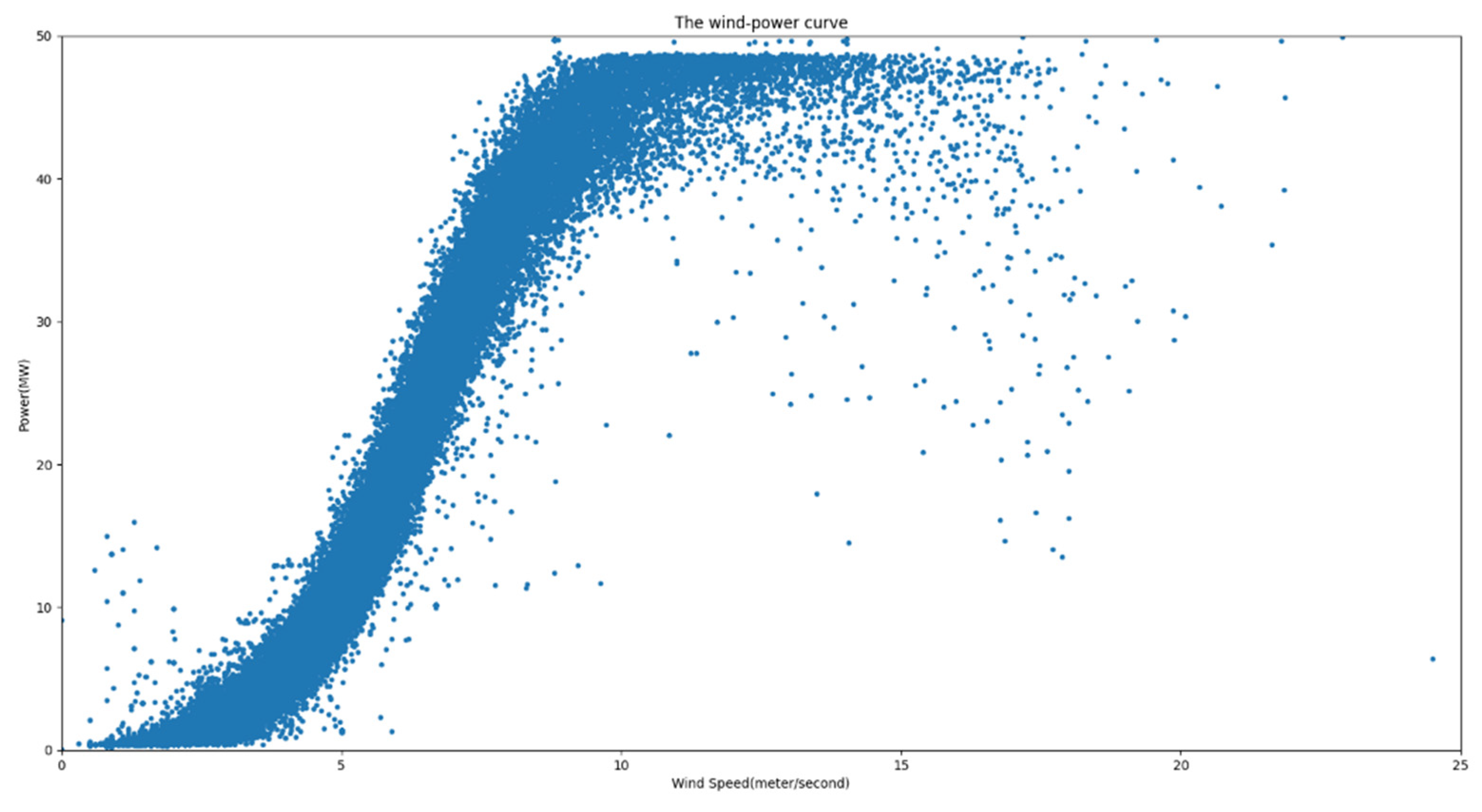
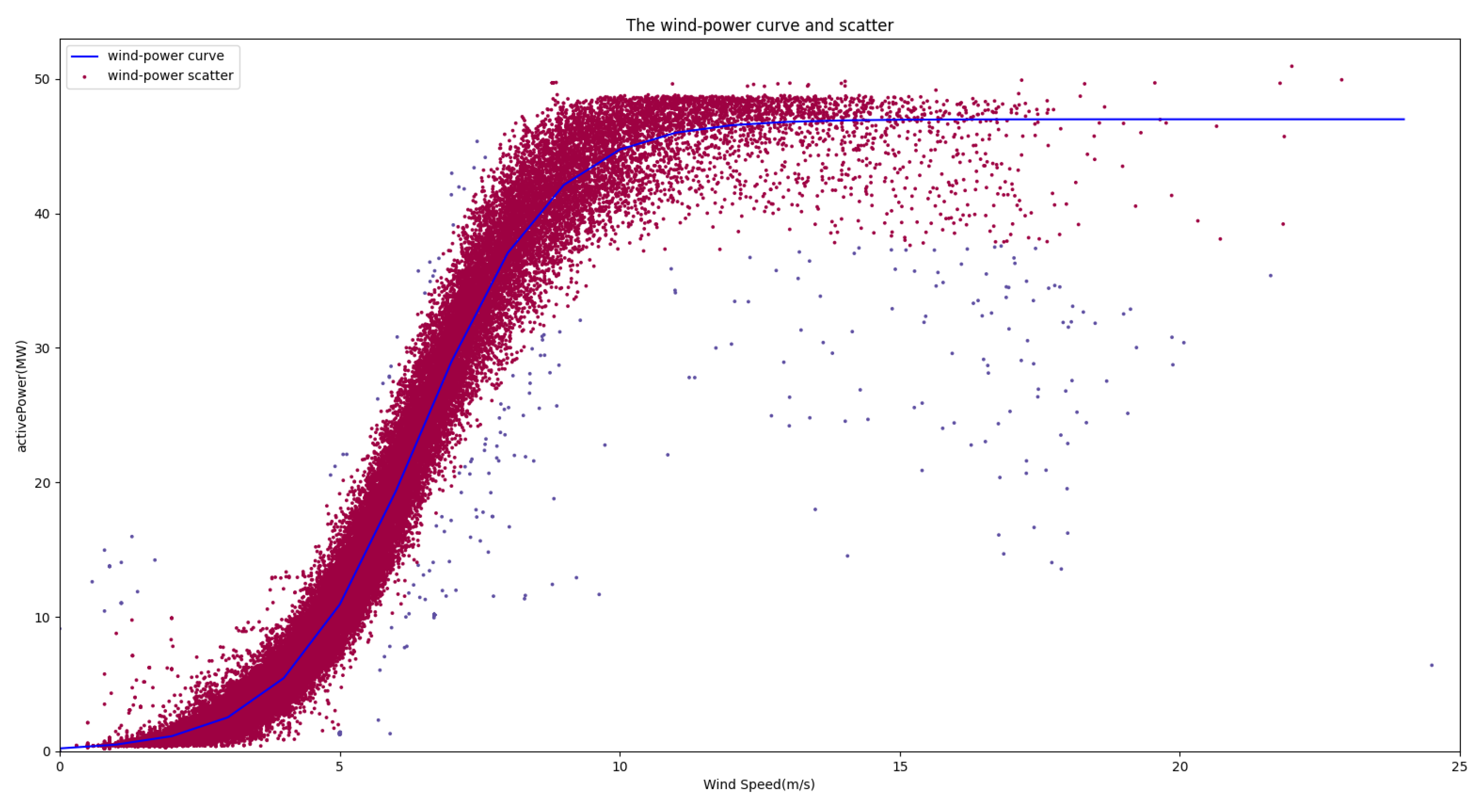
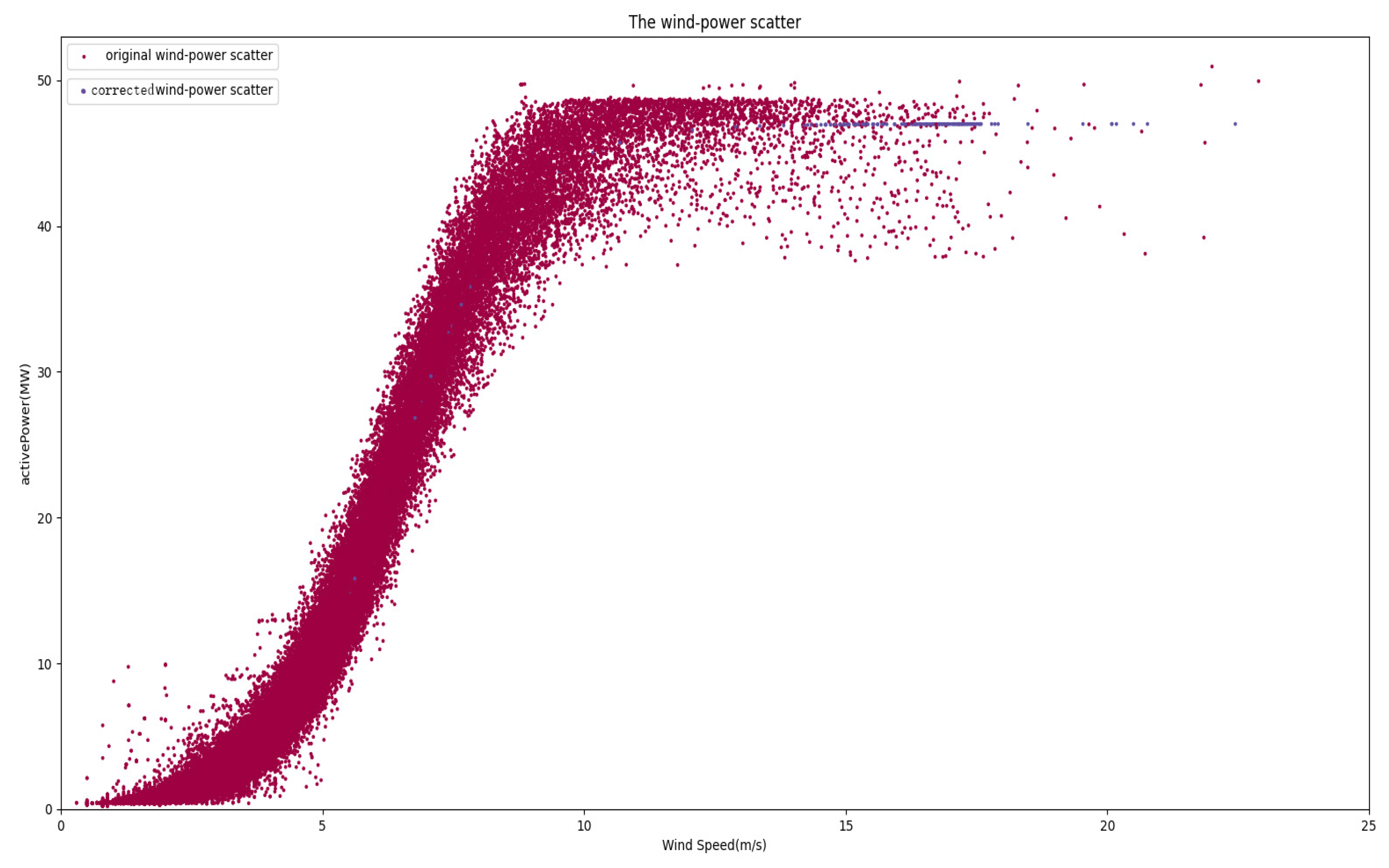
From Figure 13, it is evident that the majority of the data aligned with the wind power curve distribution. The nominal installed capacity was 48 MW. Utilizing Equation (10), parameter A was computed as 0.83735637, whereas the value of B was determined to be 6.4278509. With the derived wind power curve function, it becomes possible to employ a designated threshold (set at 0.15) for the labeling process. The outcomes of this labeling procedure are illustrated in Figure 14. The red segment represents the retained valid data, whereas the 468 instances of anomalous data have been marked.

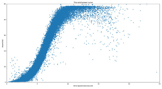
Figure 13. Wind speed–power scatter plot.

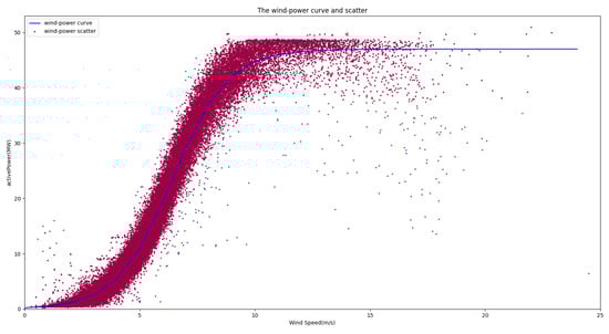
Figure 14. Data cleansing effect based on wind power curve and scatter.

For wind speed data that has undergone the labeling process, subsequent correction using linear interpolation is necessary. According to the linear interpolation formula (Equation (21)), considering a total of $n$ continuous time-series data points denoted as $x_t$, … $x_{t+i}$, … $x_{t+n}$ (where $i$ = 1, 2, … $n$ − 1), Xt + i represents unknown or anomalous values (with a maximum of $n$ − 2 unknown or anomalous values), whereas $x_t$ and $x_{t+n}$ are known values. Utilizing $x_t$ and $x_{t+n}$, interpolation was performed to supplement the data.

$$x_{t+i}=x_i+\frac{i}{n-1}(x_{t+n}-x_t)$$

(21)

where:

$x$ is the measured wind speed.

After wind speed correction, the revised power can be computed using Equation (22). From Equation (22), it is evident that $x$ and $y$ represent time-series data. Here, $x$ serves as the reference data with $N$ data points, and $y$ represents the data requiring correction, with n data points. Notably, $n$ < $N$, and the data needing correction is included within the $N$ time series.

$$\mathrm{x},y{y}_N=\overline{y_n}+r\frac{e_x}{e_y}(x_N-\overline{x_n})$$

(22)

In the formula:

$x$, $y$ is the measured power and measured wind speed of the wind farm;

$y_N$ is the Nth time series power value of the data needing correction;

$x_N$ is the Nth time series wind speed value of the reference data;

$\overline{x_n}$ is the average wind speed of n time series wind speeds of the reference data;

$\overline{y_n}$ is the average power of n time series powers of the data needing correction;

$e_x$ is the standard deviation of m time series wind speeds of the reference data;

$e_y$ is the standard deviation of m time series wind speeds of the data needing correction; and

$r$ is the correlation coefficient between n time series of the reference and corrected power data.

The scatter plot of wind speed–power after correction is illustrated in Figure 15, with blue dots representing post-correction wind speed and power data. This processed data can subsequently be utilized for dataset generation.

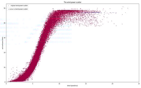
Figure 15. Corrected wind speed–power scatter plot.

Day-ahead power prediction requires predicting the power values for each 15-min interval of the morning of the upcoming day. This accounts for a total of 96 data points. Consequently, the model’s output is a power sequence with a length of 96. The available training data consists of data from the day before and days prior, encompassing both numerical forecast data and actual collected data. Within this algorithm, data from the last three days, including numerical forecast data and time data for the current day and the day after, are utilized. This results in a training dataset of 39 dimensions, each with a length of 96. To achieve optimal training efficacy, a sliding extraction approach was employed for dataset generation, leading to the creation of 55,392 sets of training data.

4.2. Augmentation and Quality Assessment of High MR Datasets

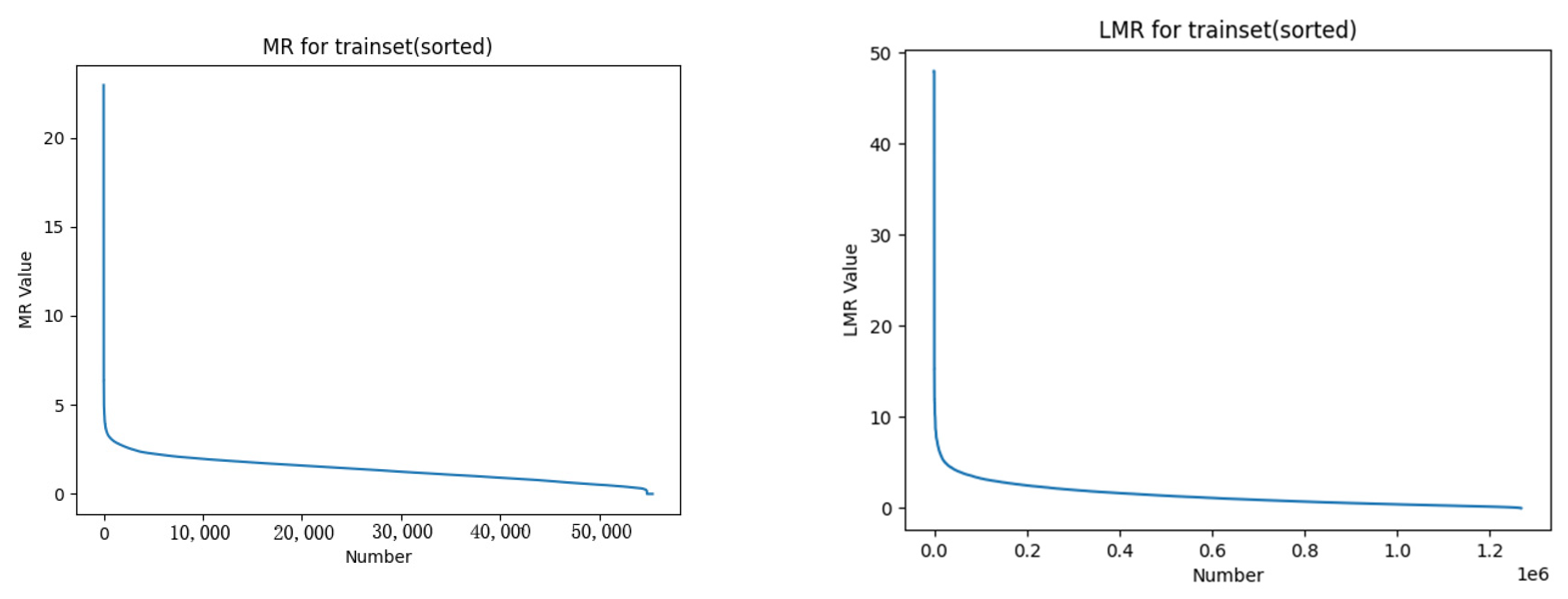
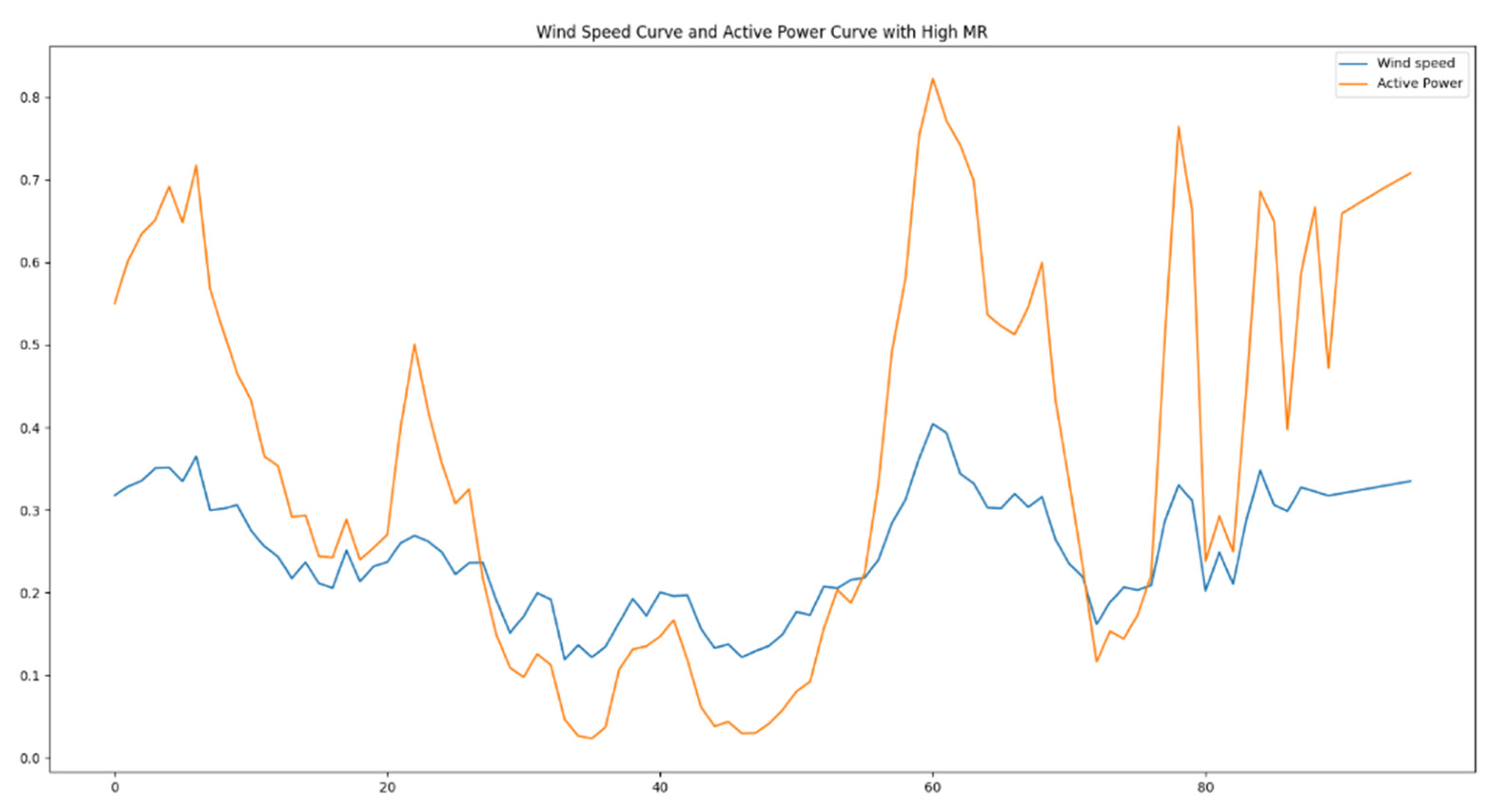
For the generated dataset of over 50,000 sets of training data, mutation rates and average mutation rates were computed according to the respective formulas. The mutation and average mutation rate curves of the training set are illustrated in Figure 16. From the graph, it is evident that approximately 1% of the data exhibited mutation rates significantly higher than the average mutation rate. Figure 17 depicts a segment of training data chosen to exhibit the high mutation rates, showcasing the wind speed and power curves. From the graph, it is evident that as wind speed experiences intense fluctuations, there are corresponding substantial fluctuations in the power output. This subset of data within the training set could impact the precision of the model’s predictions. Consequently, data augmentation is necessary for this specific subset of training data.

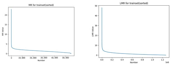
Figure 16. MR and LMR curves of the training set.

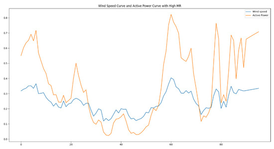
Figure 17. Wind speed and power curves with high MR.

Based on the quality assessment of generated data, an overall evaluation was conducted considering three aspects: diversity, fidelity, and effectiveness of the generated samples. Principal component analysis (PCA), a linear method, identifies a new basis with orthogonal vectors that capture the maximum variance directions in the data. We computed the first two components using real data, then projected both real and synthetic samples onto the new coordinate system (as shown in Figure 18a). Though PCA plots may not have yielded a definitive conclusion, t-distributed stochastic neighbor embedding (t-SNE) plots revealed a similar distribution pattern between the original (black) and synthetic (red) data (as depicted in Figure 18b). t-SNE is a non-linear manifold learning technique used for high-dimensional data visualization [29]. It transforms the similarity between data points into joint probabilities, aiming to minimize the Kullback–Leibler divergence between low-dimensional embedding and high-dimensional data. Figure 18 presents the outcomes of PCA and t-SNE, qualitatively assessing the similarity of distributions between real and synthetic data. Both methods exhibited strikingly similar patterns and noticeable overlaps, indicating that the synthetic data captured crucial aspects of real-data features.

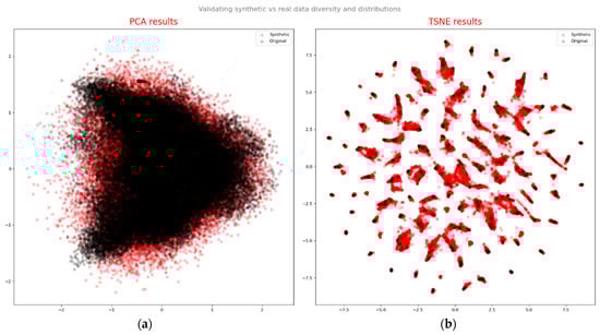
Figure 18. Validating synthetic vs. real data diversity and distributions: (a) PCA results; (b) t-SNE results.

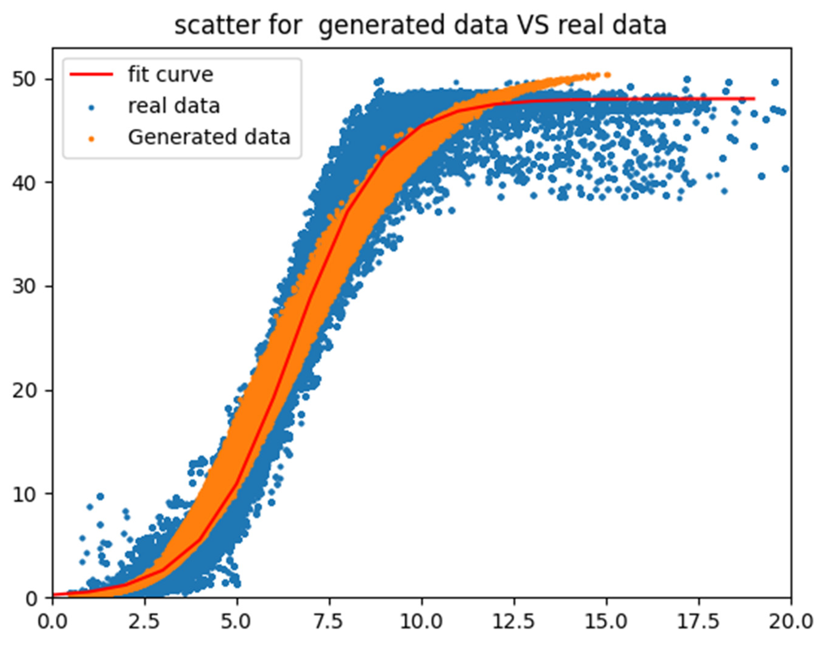
By extracting wind speed and power values from the generated dataset and overlaying them onto a scatter plot based on real data (as shown in Figure 19), we observed that the generated scatter plot broadly followed the trend of the wind speed–power curve, with the exception of an overestimation in power for wind speeds exceeding 11 m per second.

Figure 19. Scatter plot of generated vs. real data.

4.3. Power Prediction Accuracy Comparison

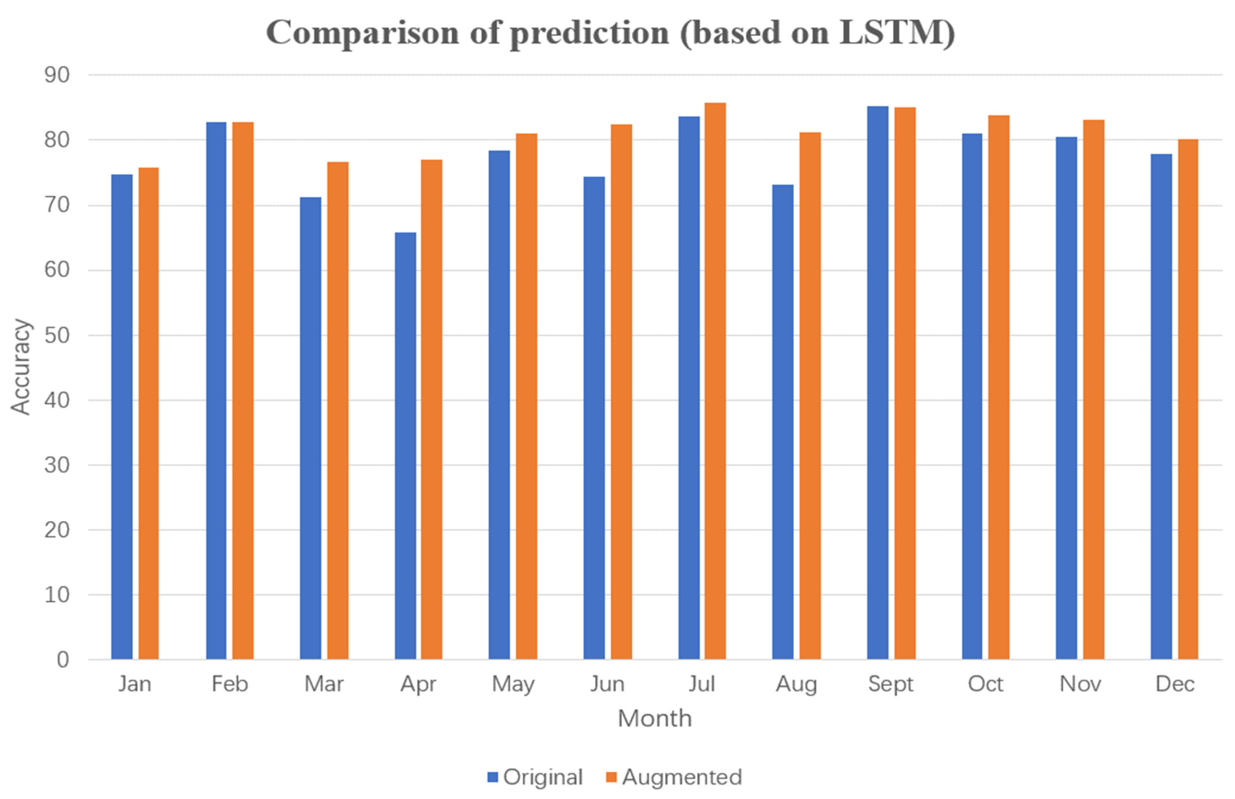
To validate the effectiveness of this framework, we selected several algorithms mentioned in Table 1, such as LSTM and DWT_AE_BiLSTM, for comparison. The comparison of their performance was conducted based on two dimensions. Firstly, the accuracy of power prediction was evaluated on a monthly basis.

From Figure 20, Figure 21, Figure 22 and Figure 23, it can be observed that after data augmentation, the LSTM algorithm achieved higher accuracy in power prediction compared with before augmentation, with an average improvement of 3.83%. Specifically, the accuracy improvement exceeded 5.43% in months 3, 4, 6, and 8, and even reached 11.1% in April.

Figure 20. Comparison of predictions (based on LSTM).

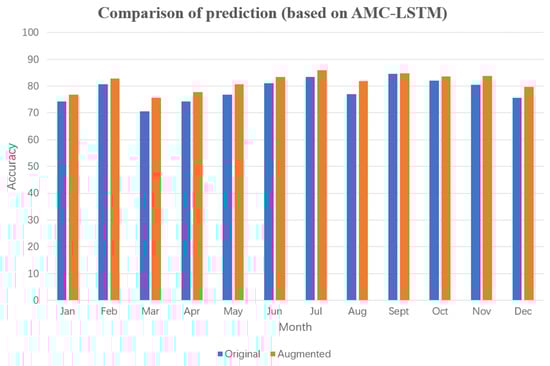
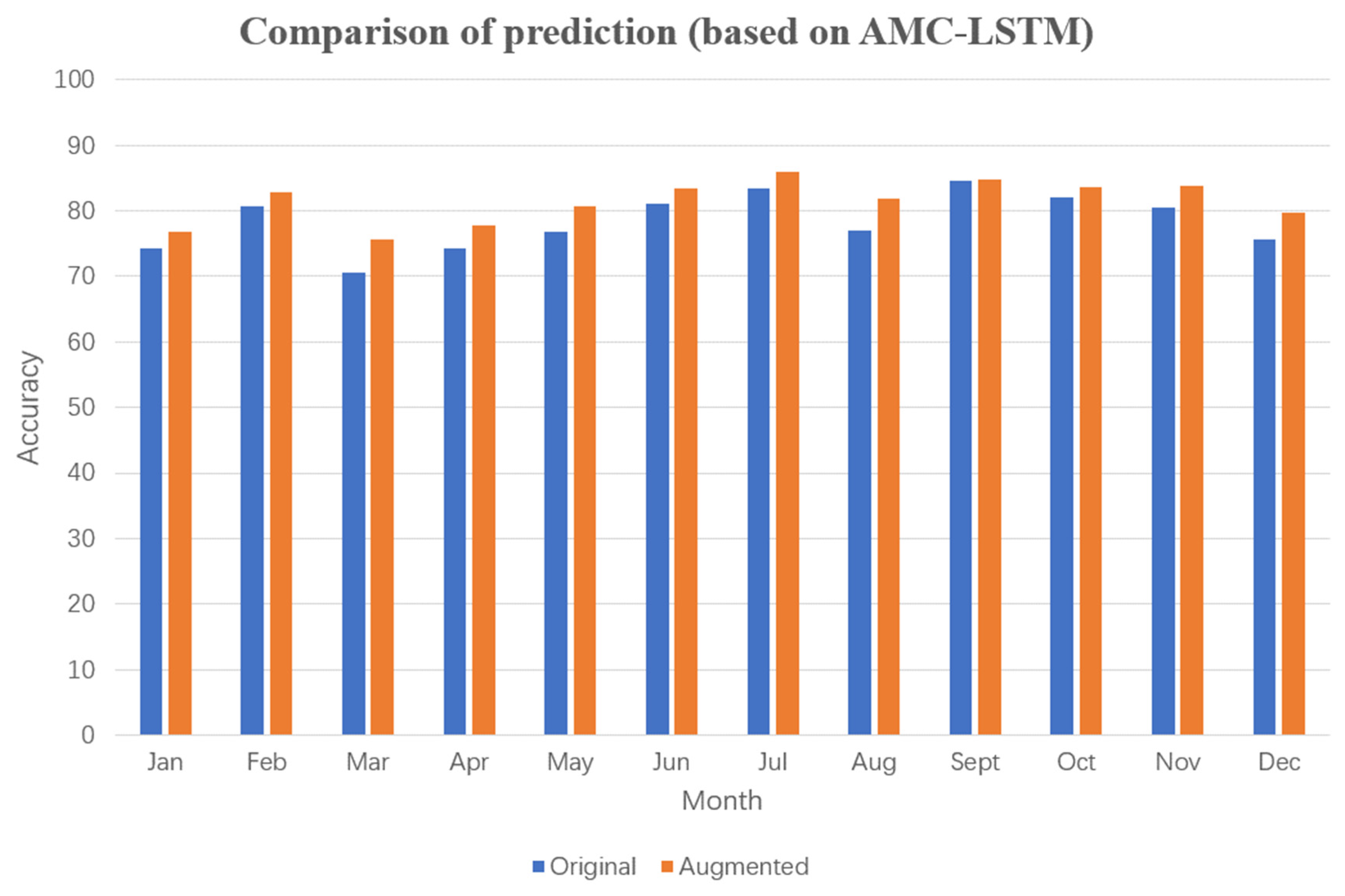
Figure 21. Comparison of predictions (based on AMC-LSTM).

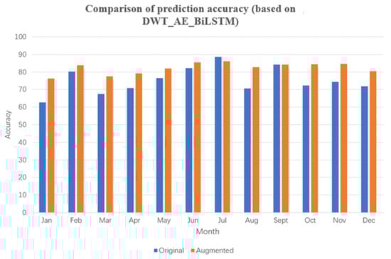
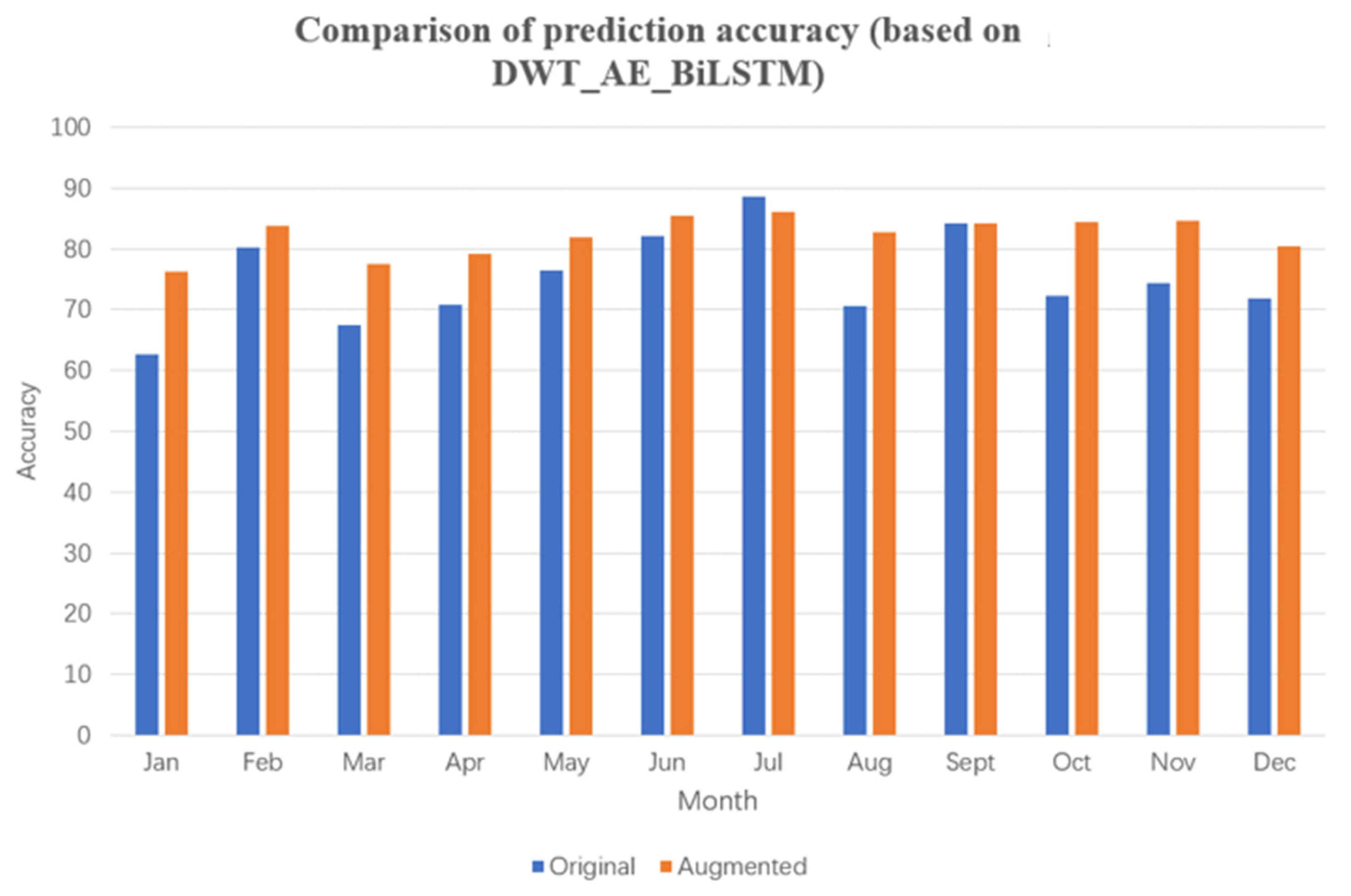
Figure 22. Comparison of prediction accuracy (based on DWT_AE_BiLSTM).

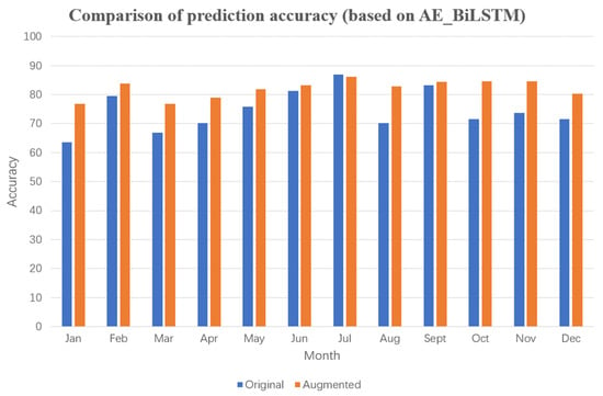
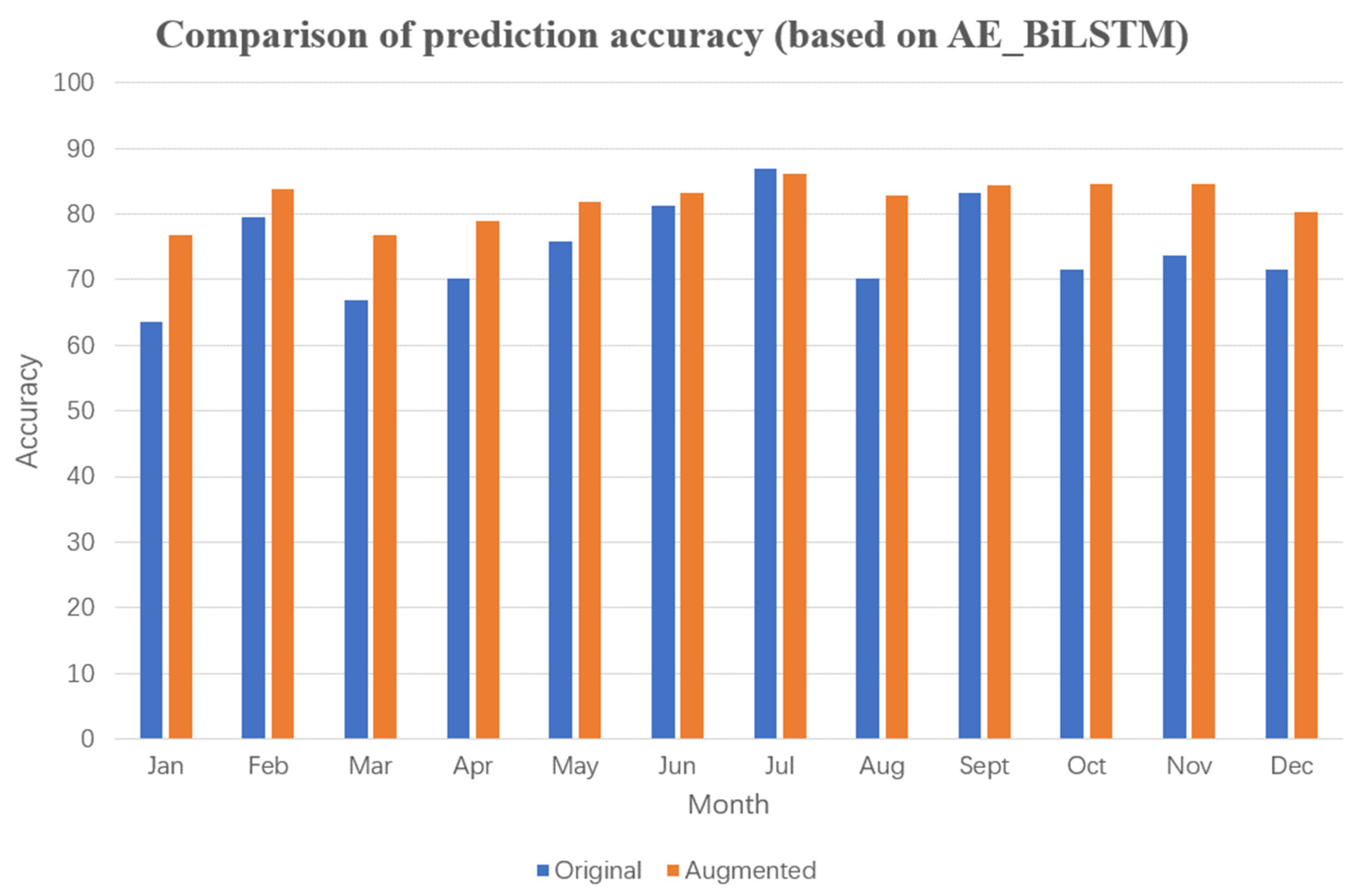
Figure 23. Comparison of prediction accuracy (based on AE_BiLSTM).

Using the AMC-LSTM algorithm for power prediction in wind farms (Figure 21 accuracy was improved by 3.02% after extracting mutation data for data augmentation, with a 5.12% improvement in March.

Furthermore, the commonly used DWT_AE_BiLSTM and AE_BiLSTM algorithms were selected for comparative experiments. After data augmentation, the average monthly improvement in prediction accuracy was 7.10 and 7.49%, respectively. These experimental results with four commonly used power prediction algorithms reveal that data augmentation through extraction of mutation data leads to significant improvement in prediction accuracy. In particular, the AE_BiLSTM algorithm, which utilizes data encoding, outperformed the LSTM algorithm in terms of prediction accuracy. However, the DWT_AE_BiLSTM algorithm, which incorporates wavelet processing, underperformed slightly compared with results without wavelet processing, which differs from findings in related literature.

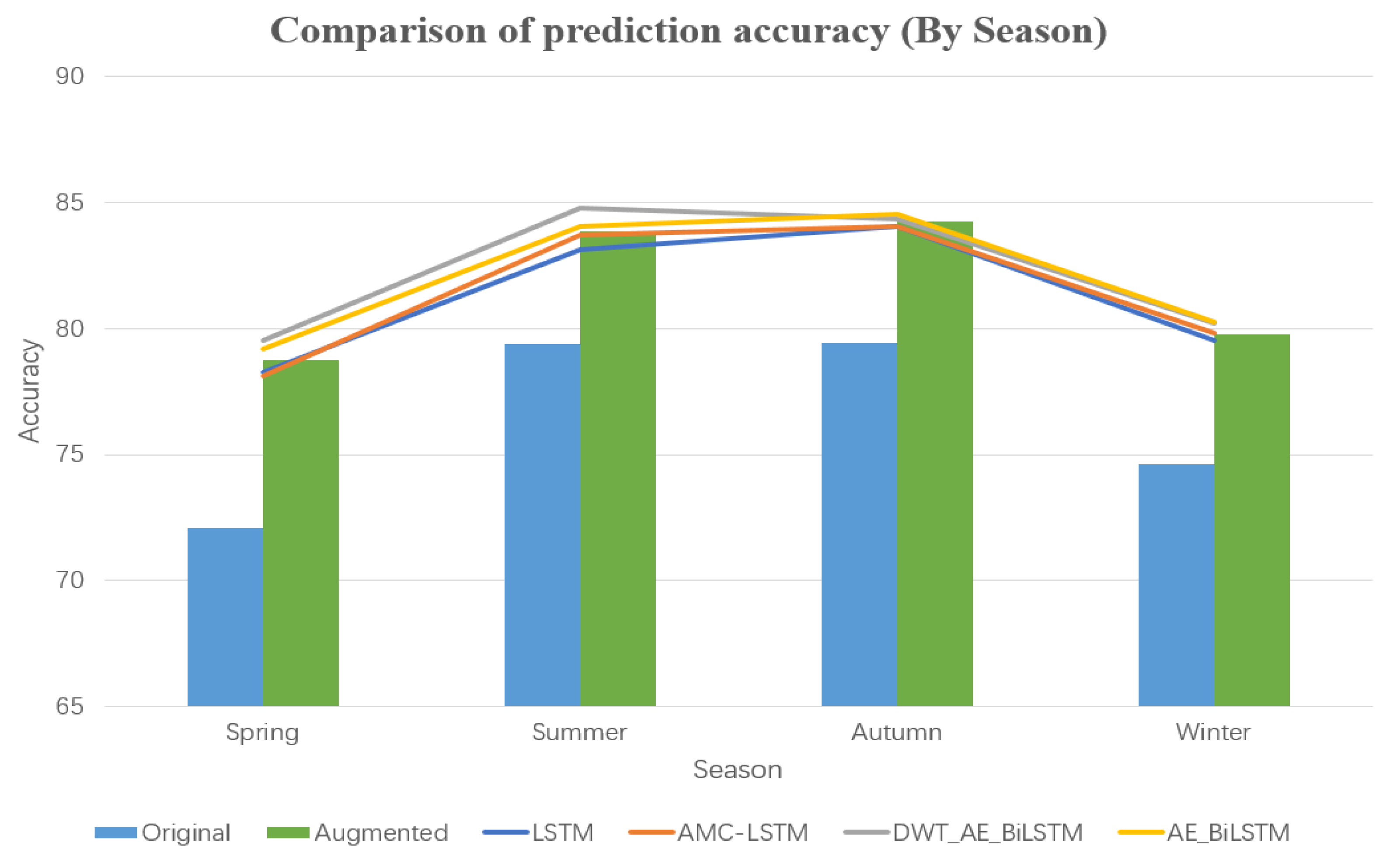
Secondly, we compared the prediction accuracy based on different seasons (Figure 24). As shown in the figure, accuracy improvement was 6.7, 4.47, 4.82, and 5.36% for spring, summer, autumn, and winter, respectively, with more prominent effects in spring and winter. The DWT_AE_BiLSTM algorithm performed well in the spring and summer seasons, but poorly in autumn and winter. Therefore, in order to achieve better short-term prediction accuracy, it is not advisable to adopt a single prediction model for the entire year. Instead, the prediction model should be selected for each season or even month to month by comparing with prediction performance in previous years.

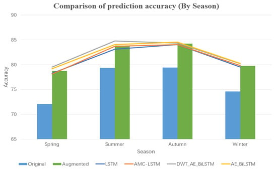
Figure 24. Comparison of prediction accuracy (by season).

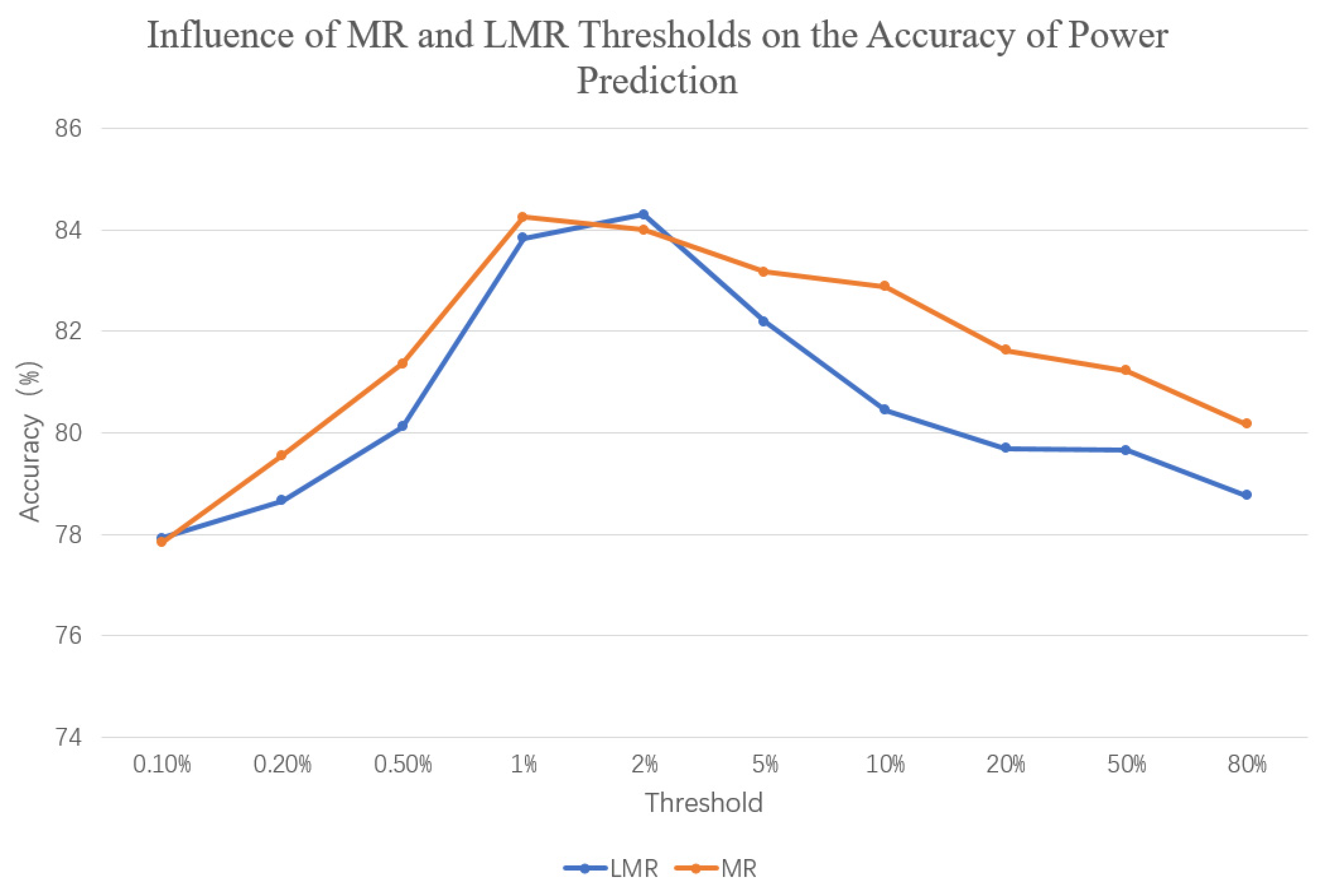
The above experiment used a mutation rate threshold of 1% to obtain the results. In order to further analyze the impact of the selection of local mutation rate (LMR) and mutation rate (MR) on prediction accuracy, the annual prediction accuracy was calculated using several thresholds: 0.1, 0.2, 0.5, 1, 2, 5, 10, 20, 50, and 80% (refer to Figure 25). From the graph, it can be observed that the selection of mutation directly affected the prediction accuracy. When the values were too small or too large, the results tended to be similar to not performing a dataset expansion. Only by selecting the appropriate threshold could a higher prediction accuracy be obtained. Using the local mutation rate as the threshold for data extraction, the same result was obtained for feedback on prediction accuracy, but the threshold for achieving maximum prediction accuracy was generally larger than the threshold for mutation rate. This is because the mutation rate (MR) averages the entire data segment, resulting in generally smaller values. In order to obtain the appropriate threshold, the following method can be used:

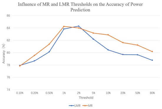
Figure 25. Influence of MR and LMR thresholds on the accuracy of power prediction.

(1)

Calculate the mutation rate and local mutation rate separately, according to Formulas (7) and (8).

(2)

Use segmented statistics of the mutation rate or local mutation rate data (e.g., regular processing) to arrange the data in descending order according to the statistical frequency.

(3)

Calculate the gradient descent maximum mutation rate as the threshold for data extraction, based on the formula:

$$gradu={\alpha }_x\frac{\partial u}{\partial x}+{\alpha }_y\frac{\partial u}{\partial y}$$

(23)

(4)

Perform data extraction based on the calculated threshold.

In summary, through the entire experimental process, it was evident that data augmentation through the extraction of mutation data led to a significant improvement in prediction accuracy regardless of the algorithm used for power prediction, with particularly notable improvements in the spring and winter. Months 1, 3, 4, and 8 showed much higher improvements compared with the other months, and these months also experience frequent weather transitions.

5. Conclusions

This research presents a data augmentation method that leverages generative adversarial networks (GANs) to enhance the accuracy of short-term wind turbine power predictions. By integrating concepts from computer science and meteorology, it introduces the mutation rate (MR) and local mutation rate (LMR) detection techniques to filter historical data based on desired mutation characteristics. The utilization of GAN-generated data, specifically focused on mutation-induced wind speed information, enriches the training sets for model optimization. In our experimental evaluations, this approach demonstrated a significant improvement in wind turbine power prediction accuracy, achieving an average monthly prediction precision about 5% higher than conventional methods. This affirms the effectiveness of harnessing mutation-derived wind speed data and GANs to enhance the reliability of predictions. It is important to note that though our proposed method achieved a 5% improvement in the wind farm used for experimentation, the impact of the approach may vary in different locations due to diverse geographical distributions and climatic variations in wind farms. Therefore, our future research efforts will involve validating the effectiveness of the method in wind farms that represent distinct geographical characteristics, such as plateaus, plains, and mountainous regions, with the aim of ensuring broader applicability of our algorithm. In summary, this study introduces a promising data augmentation technique that bridges the domains of computer science and meteorology, highlighting its potential in advancing the accuracy of short-term wind turbine power predictions. The next steps will involve further refinement of mutation rate detection and GAN model enhancement strategies.

References

- Global Wind Energy Council. GWEC Global Wind Report 2023; Global Wind Energy Council: Bonn, Germany, 2023; Available online: https://gwec.net/globalwindreport2023/ (accessed on 1 July 2023).
- REN21. Renewables 2023 Global Status Report Collection, Renewables in Energy Supply. 2023. Available online: https://www.ren21.net/gsr-2023/ (accessed on 1 July 2023).
- GB/T 40607-2021; Technical Requirements for Dispatching Side Prediction System of Wind or Photovoltaic Power. Chinese GB Standards: Guangzhou, China, 2021. Available online: http://c.gb688.cn/bzgk/gb/showGb?type=online&hcno=A86838E2F9FF5DCE3975125156E89D52 (accessed on 1 July 2023).
- Gu, C.; Li, H. Review on deep learning research and applications in wind and wave energy. Energies 2022, 15, 1510. [Google Scholar] [CrossRef]
- Higashiyama, K.; Fujimoto, Y.; Hayashi, Y. Feature Extraction of NWP Data for Wind Power Prediction Using 3D-Convolutional Neural Networks. Energy Procedia 2018, 155, 350–358. [Google Scholar] [CrossRef]
- Jiang, Y.; Chen, X.; Yu, K.; Liao, Y. Short-term wind power prediction using hybrid method based on enhanced boosting algorithm. J. Mod. Power Syst. Clean Energy 2017, 5, 126–133. [Google Scholar] [CrossRef]
- Yatiyana, E.; Rajakaruna, S.; Ghosh, A. (Eds.) Wind speed and direction prediction for wind power generation using ARIMA model. In Proceedings of the 2017 Australasian Universities Power Engineering Conference (AUPEC), Melbourne, VIC, Australia, 19–22 November 2017; IEEE: Piscataway, NJ, USA, 2017. [Google Scholar] [CrossRef]
- Cadenas, E.; Jaramillo, O.A.; Rivera, W. Analysis and prediction of wind velocity in chetumal, quintana roo, using the single exponential smoothing method. Renew. Energy 2010, 35, 925–930. [Google Scholar] [CrossRef]
- Gendeel, M.; Zhang, Y.; Qian, X.; Xing, Z. Deterministic and probabilistic interval prediction for wind farm based on VMD and weighted LS-SVM. Energy Sources Part A Recovery Util. Environ. Eff. 2019, 43, 800–814. [Google Scholar] [CrossRef]
- Xiao, Y.; Su, X.; Yuan, Q.; Liu, D.; Shen, H.; Zhang, L. Satellite video super-resolution via multiscale deformable convolution alignment and temporal grouping projection. IEEE Trans. Geosci. Remote Sens. 2021, 60, 5610819. [Google Scholar] [CrossRef]
- Xiao, Y.; Yuan, Q.; Jiang, K.; Jin, X.; He, J.; Zhang, L.; Lin, C.W. Local-Global Temporal Difference Learning for Satellite Video Super-Resolution. IEEE Trans. Circuits Syst. Video Technol. 2023. [Google Scholar] [CrossRef]
- Chen, Y.; Wang, Y.; Dong, Z.; Su, J.; Han, Z.; Zhou, D.; Zhao, Y.; Bao, Y. 2-D regional short-term wind speed forecast based on CNN-LSTM deep learning model. Energy Convers. Manag. 2021, 244, 114451. [Google Scholar] [CrossRef]
- Hu, Y.-L.; Chen, L. A nonlinear hybrid wind speed prediction model using LSTM network, hysteretic ELM and Differential Evolution algorithm. Energy Convers. Manag. 2018, 173, 123–142. [Google Scholar] [CrossRef]
- Zhao, R.; Yan, R.; Chen, Z.; Mao, K.; Wang, P.; Gao, R.X. Deep learning and its applications to machine health monitoring. Mech. Syst. Signal Process. 2019, 115, 213–237. [Google Scholar] [CrossRef]
- Jalali, S.M.J.; Ahmadian, S.; Khodayar, M.; Khosravi, A.; Shafie-khah, M.; Nahavandi, S.; Catalao, J.P. An advanced short-term wind power prediction framework based on the optimized deep neural network models. Int. J. Electr. Power Energy Syst. 2022, 141, 108143. [Google Scholar] [CrossRef]
- Ding, M.; Zhou, H.; Xie, H.; Wu, M.; Nakanishi, Y.; Yokoyama, R. A gated recurrent unit neural networks based wind speed error correction model for short-term wind power prediction. Neurocomputing 2019, 365, 54–61. [Google Scholar] [CrossRef]
- Chen, J.; Liu, H.; Chen, C.; Duan, Z. Wind speed prediction using multi-scale feature adaptive extraction ensemble model with error regression correction. Expert Syst. Appl. 2022, 207, 117358. [Google Scholar] [CrossRef]
- Wang, J.; Zhang, L.; Wang, C.; Liu, Z. A regional pretraining-classification-selection prediction system for wind power point prediction and interval prediction. Appl. Soft Comput. 2021, 113, 107941. [Google Scholar] [CrossRef]
- Xu, P.; Zhang, M.; Chen, Z.; Wang, B.; Cheng, C.; Liu, R. A Deep Learning Framework for Day Ahead Wind Power Short-Term Prediction. Appl. Sci. 2023, 13, 4042. [Google Scholar] [CrossRef]
- Xiong, B.; Lou, L.; Meng, X.; Wang, X.; Ma, H.; Wang, Z. Short-term wind power prediction based on Attention Mechanism and Deep Learning. Electr. Power Syst. Res. 2022, 206, 107776. [Google Scholar] [CrossRef]
- Khazaei, S.; Ehsan, M.; Soleymani, S.; Mohammadnezhad-Shourkaei, H. A high-accuracy hybrid method for short-term wind power prediction. Energy 2022, 238, 122020. [Google Scholar] [CrossRef]
- Huang, L.; Li, L.; Wei, X.; Zhang, D. Short-term prediction of wind power based on BiLSTM–CNN–WGAN-GP. Soft Comput. 2022, 26, 10607–10621. [Google Scholar] [CrossRef]
- Han, S.; Zhang, L.N.; Liu, Y.Q.; Zhang, H.; Yan, J.; Li, L.; Lei, X.-H.; Wang, X. Quantitative evaluation method for the complementarity of wind–solar–hydro power and optimization of wind–solar ratio. Appl. Energy 2019, 236, 973–984. [Google Scholar] [CrossRef]
- Qu, Z.; Yu, J. Quantitative Evaluation on Consistency and Complementarity of Wind Power Variability. Power Syst. Technol. 2013, 37, 7. [Google Scholar]
- Yoon, J.; Jarrett, D.; Van der Schaar, M. Time-Series Generative Adversarial Networks. In Proceedings of the Advances in Neural Information Processing Systems, Vancouver, BC, Canada, 8–14 December 2019; Volume 32. Available online: https://proceedings.neurips.cc/paper_files/paper/2019 (accessed on 15 December 2019).
- Sevlian, R.; Rajagopal, R. Detection and Statistics of Wind Power Ramps. IEEE Trans. Power Syst. 2013, 28, 3610–3620. [Google Scholar] [CrossRef]
- Jiang, K.; Wang, Z.; Yi, P.; Wang, G.; Lu, T.; Jiang, J. Edge-enhanced GAN for remote sensing image superresolution. IEEE Trans. Geosci. Remote Sens. 2019, 57, 5799–5812. [Google Scholar] [CrossRef]
- IEC 61400-12-1; Wind Turbines-Part 12-1: Power Performance Measurements of Electricity Producing Wind Turbines: Annex G. International Electrotechnical Commission: Geneva, Switzerland, 2012.
- Xiao, Y.; Yuan, Q.; Jiang, K.; He, J.; Wang, Y.; Zhang, L. From degrade to upgrade: Learning a self-supervised degradation guided adaptive network for blind remote sensing image super-resolution. Inf. Fusion 2023, 96, 297–311. [Google Scholar] [CrossRef]
Disclaimer/Publisher’s Note: The statements, opinions and data contained in all publications are solely those of the individual author(s) and contributor(s) and not of MDPI and/or the editor(s). MDPI and/or the editor(s) disclaim responsibility for any injury to people or property resulting from any ideas, methods, instructions or products referred to in the content. |
© 2023 by the authors. Licensee MDPI, Basel, Switzerland. This article is an open access article distributed under the terms and conditions of the Creative Commons Attribution (CC BY) license (https://creativecommons.org/licenses/by/4.0/).