Improved Active and Reactive Energy Forecasting Using a Stacking Ensemble Approach: Steel Industry Case Study

Abstract

The prevalence of substantial inductive/capacitive loads within the industrial sectors induces variations in reactive energy levels. The imbalance between active and reactive energy within the network leads to heightened losses, diminished network efficiency, and an associated escalation in operating costs. Therefore, the forecasting of active and reactive energy in the industrial sector confers notable advantages, including cost reduction, heightened operational efficiency, safeguarding of equipment, enhanced energy consumption management, and more effective assimilation of renewable energy sources. Consequently, a range of specialized forecasting methods for different applications have been developed to address these challenges effectively. This research proposes a stacked ensemble methodology, denoted as Stack-XGBoost, leveraging three distinct machine learning (ML) methods: extra trees regressor (ETR), adaptive boosting (AdaBoost), and random forest regressor (RFR), as foundational models. Moreover, the incorporation of an extreme gradient boosting (XGBoost) algorithm as a meta-learner serves to amalgamate the predictions generated by the base models, enhancing the precision of the active/reactive energy consumption forecasting using real time data for steel industry. To assess the efficacy of the proposed model, diverse performance metrics were employed. The results show that the proposed Stack-XGBoost model outperformed other forecasting methods. Additionally, a sensitivity analysis was conducted to assess the robustness of the proposed method against variations in input parameters.

1. Introduction

In recent times, the global population’s substantial increase has led to a notable rise in electricity demand. To meet this demand, power plants have been relying on conventional fossil fuels, such as oil, coal, and gas, for electricity generation. However, these traditional energy sources have had adverse environmental impacts due to the emission of carbon dioxide (CO₂) and other harmful gases, contributing to global warming [1]. Consequently, urgent actions from researchers, governments, and policymakers are imperative to explore alternative sources and promote their implementation. Renewable energy sources (RES), including windmills and solar photovoltaic (PV), present viable alternatives to conventional energy [2,3]. As a result, embracing RES and electric vehicles (EVs) emerges as an ideal solution to address these pressing challenges. Nevertheless, the increasing number and variety of electronic devices have posed challenges in efficiently connecting each customer’s active and reactive power demand [4]. In contemporary power systems, persistent challenges involving periodic and structural power shortages in addition to significant peak–valley disparities have endured over short periods. These issues have raised concerns regarding resource depletion and the necessity to bridge the gap between power generation and consumption [5,6]. However, In light of the fourth industrial revolution, businesses have realized that integrating Industry 4.0 solutions confers competitive advantages and fosters opportunities for enhanced sustainable management [7,8]. Therefore, real-time data gathering and predictive analytics are harnessed through big data analytics and Artificial Intelligence (AI) and forecasting methodologies [9]. Hence, the introduction of active and reactive energy forecasting has been employed to address these specific challenges, particularly within the industrial sector, where the prevalence of inductive and capacitive loads surpasses that of the residential sector. These techniques address the modern industrial demands, encompassing aspects like flexibility, heightened productivity, improved market demand forecasting, optimization of resources within and beyond industrial units, and promoting sustainable manufacturing processes [10].

Numerous prior studies have addressed the forecasting of energy consumption demand. To accomplish this task, diverse methodologies have been employed, encompassing statistical, machine learning (ML), and deep learning (DL) techniques [11]. The selection of these methods is contingent upon the specific characteristics and requirements of each problem, leading to the consideration of distinct forecasting periods, namely, short, medium, and long-term horizons, depending on the application at hand. Regarding statistical methods, the authors in [12] utilized an autoregressive moving average approach to predict the electric arc furnace reactive power demand. Moreover, the work in [13] introduced a mixed regression clustering methodology for medium-term reactive power forecasting (spanning one month to a year ahead) in transmission grids. Furthermore, the work in [14] presented a generalized additive model for short-term reactive power forecasting at the interface between distribution and transmission grids. In addition, different statistical methods, including linear regression [15], K-nearest neighbors (KNN) [16], and CUBIST [17], were employed to forecast energy consumption. According to [17], compared to other models, such as KNN and liner regression, the results revealed that the CUBIST attained the best performance by achieving the lowest error value when applying it on data for small-scale steel industry in South Korea. The proposed statistical models exhibited promising results, especially for substations with reactive power behaviors characterized by low variability. However, despite applying statistical methods for active/reactive energy demand forecasts, these techniques, grounded in mathematical statistics, demonstrate limited robustness and accuracy when dealing with intricate non-linear systems [18].

AI technologies based on data-driven ML techniques are employed to cope with the drawbacks of statistical methods by producing adaptable predictions that highlight the non-linear correlation between features and potential outcomes. For example, single ML models were proposed in order to address the active power consumption problem. In [19], an RF was proposed for short-term energy consumption prediction in multiple buildings. The outcomes indicate that the RF model surpassed other models, exhibiting superior performance with approximately 49.21% and 46.93% lower mean absolute error (MAE) and mean absolute percentage error (MAPE), respectively, in comparison to alternative models, including random trees. In addition, limited works take into account the forecasting of reactive energy consumption. For instance, a support vector machine (SVM) was used in [20] to forecast the grid reactive power one day ahead, whereas a Fuzzy logic was proposed in [21] to predict the wind farm reactive power one hour ahead. Further, seven different ML models were proposed in [22] to forecast energy demand for building heating systems. The results disclosed that the Extreme Learning Machine (ELM) surpassed the other model in performance. However, single models showed a deficiency compared to the hybrid ML models in forecasting active/reactive energy consumption, as stated in [23]. Hence, hybrid ML models were employed to attain better results. A hybrid ML prediction model Jaya-ELM with online search data was employed in [24] to forecast residential electricity consumption. The proposed Jaya-ELM model, incorporating online search data, exhibits noteworthy reductions of 34–51.2%, 43.03–53.92%, and 41.35–54.85% in Root Mean Squared Error (RMSE), MAPE, and MAE, respectively, when compared to other benchmark models. In addition, three occupancy estimation algorithms based on ML, including decision tree, SVM, and artificial neural networks (ANN), have been chosen and assessed for their ability to accurately estimate occupancy status during each season of a building energy model [25]. The building energy simulation, validated using estimated occupancy data, demonstrated a notable enhancement in the accuracy of energy consumption estimation, and it exhibited a close alignment with the actual energy usage profiles. Finally, an ensemble learning technique, referred to as ‘Ensemble Bagging Trees’ (EBT), is employed, utilizing data derived from meteorological systems as well as building-level occupancy and meters for energy demand forecast for residential buildings [26]. The results demonstrated that the proposed EBT model achieved enhanced accuracy in predicting the hourly energy demand of the test building, as indicated by the MAPE, which ranged from 2.97% to 4.63%. Although ML models are extensively employed for active/reactive energy forecasting, nevertheless, they encounter challenges such as nonlinear relationships, high-dimensional data, temporal dependencies, seasonal patterns, the interpretability of models, their generalization capability, and issues related to scalability [27].

However, due to the integration of automated meters, the electrical companies are capable of monitoring the dynamic variations in active/reactive power requirements, thereby accessing abundant and updated data streams. Consequently, DL models have been posited to address the challenges encountered by ML models. Various applications of DL models for active/reactive energy predictions are made possible by high-resolution measurements [10]. Models based on DL capture complicated time-series features and produce adaptable forecasting by leveraging sophisticated computational capabilities and processing inclusive data inputs. Single DL methods were used to address this issue. For example, in [28], a one-dimensional convolutional neural network was presented to forecast the wind farm reactive power resolving the delay duration of static VAR compensators. The forecasting of the reactive load using dual input LSTM was addressed in [29], where the results revealed that accurate prediction of reactive load at each bus help to fine control of reactive voltage. Hybrid DL models were also proposed to cope with the energy demand problem when it comes to enormous and complicated datasets [30]. For example, a DL model based on LSTM and autoencoder was proposed in [31] to predict the electric energy consumption for a household one hour ahead. The proposed model managed to attain the lowest MAE and MSE with a value of 0.3953 and 0.3840, respectively. Additionally, multistep short-term electricity load forecasting utilizing a Residual Convolutional Neural Network (R-CNN) with a multilayered Long Short-Term Memory (ML-LSTM) architecture was employed in [32]; the results showed that the proposed model outperformed the other models since the R-CNN layers are employed to extract spatial features, while the ML-LSTM architecture is integrated for sequence learning. Another DL model based on CNN-LSTM was used in [33] and validated using a household dataset. A landmark-based spectral clustering (LSC) along with CNN-LSTM was proposed in [34] to predict the household energy consumption in power grids. The results prove that the proposed LSC-CNN-LSTM surpasses other models by achieving the lowest RMSE and MAE values of 17.54 and 9.74, respectively. While DL models have demonstrated proficiency in active/reactive energy forecasting, several challenges are encountered in utilizing them for reactive energy prediction. These encompass the requirement for abundant labeled data, the risk of overfitting due to intricate model architectures, complexities in deciphering model decisions, and the considerable computational resources essential for training and deployment [35].

Table 1. A comprehensive summary of the recent works regarding forecasting active/reactive energy.

Methodology	Reference	Model	Input Parameters	Output Resolution	Dataset	Sensitivity Analysis	Application Areas
Statistical	[12]	ARMA	Three-phase supply voltages and currents	Half-cycle	Mobarakeh steel industry	×	Industry
	[13]	A mixed regression clustering	Historical data for active and reactive power	1 month to a year ahead	National transmission grid		Transmission Grids
	[14]	Generalized Additive Model	Active and reactive power in addition to weather data	One to two days ahead	Grid data		Distribution and Transmission Grid
	[17]	CUBIST	Active and reactive energy, CO2, power factor	One hour ahead	small-scale steel industry		Industry
Machine Learning	[19]	RF	Historical data for active energy consumption	One hour and one day ahead	5 different building datasets		Buildings
	[20]	SVM	Current, voltage, load active power, and load reactive power	One day ahead	From Energy Management System (EMS)		Grids
	[37]	Ensemble neuro-fuzzy	Historical load data and the temperature		A real load profile in Iran
	[21]	Fuzzy logic	Actual voltage and current		Manjil wind farm		Wind farm
	[22]	ELM	Weather data, indoor temperature, time data	40 min ahead	Office building dataset		Buildings
	[24]	Jaya-ELM with online search data	Historical residential electricity consumption and online search data	-	Residential electricity consumption dataset
	[26]	Ensemble Bagging Trees	Metrological data, electricity data, time of the day, type of load, and workday type	One day ahead	building energy management system (BEMs) of Rinker Hall
Deep Learning	[28]	1D-CNN	Actual voltage and current	Extremely short t ≤ 0.02 s	Manjil wind farm		Wind farm
	[29]	DL-LSTM	Historical active/reactive data and workday type	15 min ahead	The power grid in Hainan Province		Grids
	[31]	LSTM and autoencoder	Global active/reactive power, global intensity, voltage, sub-metering 1, 2, and 3	One hour ahead	Household electric power consumption (IHEPC)		Buildings
	[32]	R-CNN with ML-LSTM		One hour and a day ahead	IHEPC and commercial PJM datasets
	[33]	CNN-LSTM		1 min, 1 h, 1 day, and 1 week ahead	IHEPC
	[34]	LSC-CNN-LSTM		One hour ahead
Stack model	Current study	Stack-XGB	Active and reactive energy, CO2, lead and lag power factor, load type, workday type, number of seconds from midnight	15, 30, and 60 min ahead	Steel industry	SRC and KTC	Industry

summarizes the recent works that consider forecasting the active/reactive energy using different ML and DL models. According to Table 1, it can be observed that the majority of preceding studies in the realm of ML ensemble models have predominantly addressed the prediction of active and reactive energy consumption through the lens of a regression task [12,13,14,17]. This has been accomplished by leveraging statistical models and incorporating RF methodologies at the foundational level [19]. Still, the intrinsically dynamic character of active/reactive energy consumption time-series data, intertwined with its intricate reliance on various parameters and autoregressive tendencies, engenders substantial complexity in prognosticating it via singular computational intelligence techniques, such as a standalone ensemble model [20,21,22]. In addition, these techniques prove inadequate in discerning nonlinear behavior intrinsic to time-series data, subsequently leading to diminished predictive efficacy. Moreover, the employment of DL was used to solve these problems. Nevertheless, these techniques showed a promising result, but these approaches have a complex architecture and demands enormous computer resources such as CNN [28], LSTM [29], and the combination between them [32,33,34]. Furthermore, it is noteworthy that a substantial portion of prior research efforts has mostly centered around datasets pertaining to residential contexts [36]. Surprisingly, scant attention has been directed towards industrial settings, despite the fact that industrial operations typically involve significantly elevated levels of active/reactive energy consumption owing to the utilization of diverse machinery and equipment. Thus, the consequential implications of effectively managing such energy consumption in the industrial sector to curtail expenses have been overlooked. Finally, the statistical test in order to evaluate the model’s sensitivity have been overlooked in most of the previous work.

To surmount these inherent constraints, the present research endeavored to transcend the established norm by embracing an enhanced approach—utilizing a one-level stacked ensemble model. This ensemble configuration incorporates the Adaboost, ETR, XGBoost, and RFR models, amalgamating their distinct strengths to counteract the multifaceted challenges posed by the intricate and nonlinear nature of energy consumption data. This strategic approach promises to yield enhanced predictive accuracy and reliability in forecasting. In this work, ETR’s inherent capability to grasp intricate data patterns in active/reactive energy consumption forecasting was harnessed. AdaBoost, renowned for its competence in handling prediction tasks with minimal bias errors and adeptly avoiding overfitting during training, was also incorporated. Furthermore, the study leveraged the advanced fitting proficiency of RFR and its remarkable resilience to low-information scenarios, where the XGBoost was employed to amalgamate the predictive outputs of each underlying model. The integration of XGBoost in the role of a meta-learner not only facilitated the aggregation of individual model predictions but also encompassed the quantification of model-specific errors and the uncertainty stemming from data noise. As a result, the collaborative utilization of these techniques culminated in significantly enhanced forecast accuracy. In this context, the distinctive contributions of this study, when juxtaposed with earlier research endeavors, can be succinctly summed up as follows:

• A stacking ensemble model, denoted as Stack-XGBoost, was meticulously formulated to serve as a foundational framework for active/reactive energy consumption forecasts. This model is designed to facilitate predictions for time horizons of 15 min, 30 min, and one hour ahead. It leverages a modest-sized dataset from the steel industry, with minimal hyperparameter tuning requirements.
• The efficacy of the proposed Stack-XGBoost model was assessed through a comprehensive performance evaluation using real-world data from the steel industry.
• The performance of the proposed Stack-XGBoost model was benchmarked against various proposed models using diverse sensitivity metrics, demonstrating its superior robustness and efficacy.

The paper’s organization is structured as outlined below: Section 2 elucidates the data preparation and analysis of key parameters. Section 3 expounds on the methodology for the proposed Stack-XGBoost model, addressing the forecasting of active/reactive energy consumption. Section 4 provides an in-depth exploration of results and discussions, juxtaposing the proposed Stack-XGBoost with alternative models. Finally, Section 5 presents the paper’s conclusions.

2. Data Preparation and Key Parameters Analysis

This part of the paper demonstrates the data preparation and key parameters for the used dataset, in addition to comprehensive analysis regarding the interactions between the parameters and their impact on the active and reactive energy consumption. Finally, the section elaborates the performance metrices that are employed to assess the efficiency of the developed model.

2.1. Data Partitioning

Data preparation and partitioning have been verified to positively impact model convergence. The process encompasses several steps, including data collection, organizing inputs and outputs, segmentation, and standardization using various techniques. The dataset was compiled during a one-year period from 1 January 2018 to 31 December 2018, with a 15 min interval, sourced from DAEWOO Steel Co., Ltd. in Gwangyang, South Korea [38]. This company is engaged in the production of multiple types of coils, steel plates, and iron plates. The energy consumption data is stored in a cloud-based system, accessible through the website of the Korea Electric Power Corporation, Naju-si, Republic of Korea (pccs.kepco.go.kr) [39], which provides perspectives on daily, monthly, and annual energy consumption figures. Moreover, the energy consumption data for the steel industry’s machine equipment is collected through smart meters, with supplementary details on energy consumption also being stored in a cloud-based system. The key parameters are encompassed in the dataset, which include variables such as active energy consumption ($E_{P })$, leading reactive energy ($E_{+Q })$, lagging reactive energy ($E_{-Q })$, leading power factor (${PF}_{+})$, lagging power factor (${PF}_{-}),$ CO₂ information (t[CO₂]), load type, number of seconds from midnight ($t$), day of the week, and week status.

The objective is to forecast the active and reactive energy (the lag and lead); hence, the samples are averaged and scaled based on the proposed forecasting horizon (half and one hour). Furthermore, the dataset is partitioned into distinct training and testing sets, maintaining an 80:20 ratio. Eventually, data normalization was achieved through the utilization of the standard deviation. The progression of these procedural stages is delineated by the subsequent Equations (1)–(4). Equation (3) represents the pre-training standardization of the data, and Equation (4) incorporates the difference between the actual data forecasted to assess the testing effectiveness in relation to the trained network.

$$\mu =\frac{1}{N}\sum _{i=1}^N{E}_i$$

(1)

$$\sigma =\sqrt{\frac{{\sum }_{i=1}^N{(E_i-\mu )}^2}{N}}$$

(2)

$$Z=\frac{(E_i-\mu )}{\sigma }$$

(3)

$$\overline{Z}=\sigma ·Z_{ }+\mu$$

(4)

where the symbol μ represents the mean, the energy is represented by $E_i$, and σ denotes the standard deviation of the dataset under consideration. Moreover, $N$ corresponds to the size of the dataset, whereas $E_i$ signifies the value of each energy point within the dataset. Finally, $Z$ represents normalization of the data point while the original value of the data point can be represented by $\overline{Z}$.

2.2. Principal Component Analysis

This section focuses on examining the interrelationships among the variables within the dataset. To commence, the correlation between active energy consumption and lagging reactive energy consumption is notably strong at 0.9, as depicted in Figure 1. Furthermore, a substantial correlation is observed between CO₂ emissions and active energy consumption, registering a value of 0.9, along with a value of 0.89 in relation to lagging reactive energy consumption. The correlations among the remaining variables exhibit weaker associations. Notably, the correlation between leading and lagging reactive energy consumption is distinctly high yet negatively oriented, standing at −0.94. To provide further clarification, Figure 2 illustrates the positive correlation between active energy and lagging reactive energy. This signifies that, when one of these factors increases, the other also tends to increase, and conversely, when one decreases, the other follows suit. In contrast, a weak correlation between active energy and leading reactive power is observed, indicating a negative relationship between these two variables. Figure 3 illustrates the interdependence between leading and lagging reactive energy. As discernible from the graphical representation, these two forms of reactive energy demonstrate inverse relationship. This signifies that an elevation in leading reactive energy corresponds to a reduction in lagging reactive energy, and vice versa. Furthermore, Figure 4 elucidates the operational intricacies of both reactive energy categories within a single day. For example, when lagging reactive energy attains a non-zero value, leading reactive energy remains at zero, and vice versa. In conclusion, Figure 5 conclusively demonstrates a direct correlation between CO₂ emissions and both active energy and lagging reactive energy. This observation signifies that elevated active energy consumption leads to increased CO₂ emissions into the atmosphere, primarily driven by the higher levels of active energy generation from conventional power plants.

Figure 6 presents the utilization profiles for both active energy consumption and lead/lag reactive energy consumption. Evidently, the factory initiates its operations at approximately 8 AM and concludes them around 8 PM on a daily basis. Concerning active energy consumption, Figure 6a portrays distinct consumption trends across the whole period. Consumption ascends notably between 8 AM and 12 PM, as well as from 2 PM to 5 PM. It is noteworthy that the factory remains operational even during the weekend, with Saturday exhibiting a consumption peak at 4 PM. In the context of lead reactive energy, as depicted in Figure 6b, a divergent pattern emerges. Particularly, days like Saturday and Sunday manifest heightened lead reactive energy, primarily attributed to the activation of specific capacitive load equipment and machinery. Contrarily, the behavior of lagging reactive energy showcases elevated consumption on Sunday, Tuesday, and Monday, and that can be interpreted by using different inductive load on these specific days. During days characterized by active lead reactive energy, such as Monday, Tuesday, Wednesday, Thursday, and Friday, the lagging reactive energy remains negligible. In the case of the lagging reactive energy, the lagging reactive energy appears to be high in the morning around 9 AM and during the period of 11 AM to 12 PM during the weekdays, as shown in Figure 6c. While the lagging reactive energy is linked to inductive loads and may lead to voltage reduction and decrease operational efficiency, leading reactive energy is introduced through shunt capacitors installation and has the potential to enhance the overall efficiency of the electrical system, particularly in terms of the power factor. Finally, in the realm of industrial and commercial domains, it bears significance to emphasize the imperative of adept reactive energy management and optimization. This endeavor holds the potential to substantially enhance energy efficiency while concurrently curtailing operational expenses. In general, a prevailing scenario entails lagging reactive energy, a consequence primarily attributable to the prevalence of inductive loads inherent to these environments. However, it is pivotal to recognize that both lagging and leading reactive energy can give rise to multifaceted challenges, encompassing concerns pertaining to equipment efficacy, energy expenditure, and the overarching stability of the system.

2.3. Forecast Model Performance Indices

Equations (5)–(8) are employed to assess the predictive accuracy of all models with respect to active/reactive energy. These evaluation metrics offer insight into various facets of forecast accuracy. For instance, Equation (5) delineates the computation of the Root Mean Square Error (RMSE), serving as the initial measurement criterion. Equation (6) expounds upon the Mean Square Error (MSE), while Equations (7) and (8) elucidate the calculation of the Coefficient of Determination (R²) and the Mean Absolute Error (MAE) in sequence.

$$RMSE=\sqrt{\frac{1}{N}\sum _{i=1}^N{(\widehat{E_i}-E_i)}^2}$$

(5)

$$MSE=\frac{1}{N}\sum _{i=1}^N{\left(\widehat{E_i}-E_i\right)}^2$$

(6)

$$R^2=1-\frac{{\sum }_{i=1}^N{\left(\widehat{E_i}-E_{avg}\right)}^2}{{\sum }_{i=1}^N{\left(E_i-E_{avg}\right)}^2}$$

(7)

$$MAE=\frac{1}{N}\sum _{i=1}^N|(\widehat{E_i}-E_i)|$$

(8)

where $N$ represent to the size of the dataset, and it is notable that the variables denoted as $E_i$ and $\widehat{E_i}$, respectively, embody the actual and prognosticated values, whereas $E_{avg}$ signifies the average of the actual values.

3. The Proposed Forecast Models

This section of the study reveals the developed methodology and, in addition, provides a comprehensive account of the development process of the Stacking-XGBoost model. Subsequent to the construction of the Stacking-XGBoost model, its validation will be carried out using a small-scale steel industry dataset. Furthermore, the model’s performance will be evaluated utilizing applicable performance indices to validate the effectiveness of each proposed model. The methodologies employed in this work are delineated within this section. This approach assesses and classifies supervised learning methodologies across various independent variables, classifying them into three distinct groupings. These groupings encompass bagging and boosting ensemble strategies, in addition to the Stack-XGBoost model proposed for this study. The concept of an ensemble of regressions endeavors to construct a further effective model through an amalgamation of outcomes derived from multiple regression models. In addition, bagging ensembles serve to curtail model variance while concurrently training subordinate models in parallel. Within this context, the ETR and the RFR stand as predominant manifestations of bagging methodologies. The ensemble boosting techniques strive to mitigate model bias through a progressive process of training multiple models to augment each preceding one. The AdaBoost and XGBoost stand out as the most prevalent exemplars among the prevailing boosting methods.

3.1. Random Forest Regressor

The RFR represents an ensemble-based ML technique rooted in the bagging paradigm, orchestrating the fusion of numerous trees. Within the RFR framework, a voting mechanism is harnessed to enhance the performance of multiple foundational learners, particularly decision trees (DT) in that specific research. This approach boasts distinctive attributes, including bootstrap sampling, randomized feature selection, out-of-bag error estimation, and the construction of full-depth decision trees [40,41]. The RFR is assembled from an ensemble of decision trees, wherein classification and regression trees notably benefit from this association. In tandem with the RFR, the classification and regression trees methodology experiences augmentation. Remarkably, the RFR obviates the necessity for cross-validation due to its inherent capability to function out-of-bag error approximation through the forest construction procedure. It is posited that the impartiality of out-of-bag error valuation holds true throughout a multitude of testing scenarios.

The training procedure of an RFR can be succinctly outlined as follows. The RFR draws a bootstrap sample from the original dataset in the initial stage. Subsequently, each bootstrap sample acquired in the first phase proceeds to construct an unpruned regression tree, incorporating the subsequent adjustments in the subsequent phase. A random subset ($n$) of input variables is considered at each decision node, from which the optimal split among them is determined. This process of sampling and splitting is iteratively repeated across successive nodes. This iterative process persists until the stipulated number of trees has been generated. Finally, when making predictions on new data, the RFR aggregates the forecasts of all the generated trees, resulting in an averaged prediction.

Nonetheless, the process of identifying an optimal arrangement of if-statements that align with the logged data is referred to as model improvement or training. Therefore, training involves an optimization procedure with an objective function aimed at minimizing a disparity among a forecasted value, denoted as ${\mathrm{f}}_n({\mathrm{x}}_i;{\theta }_n)$, and the actual recorded values $E_i$ as described in Equation (9).

$${\mathrm{O}\mathrm{F}}_{RFR}=\underset{\theta }{\min } {{\sum }_i({\mathrm{f}}_n({\mathrm{x}}_i;{\theta }_n)-E_i)}^2$$

(9)

The choice for ${\mathrm{f}}_n({\mathrm{x}}_i;{\theta }_n)$ typically involves calculating the mean of the records that satisfy a specific if-statement condition. A valid concern can arise regarding how to prevent the model from generating an excessively long if-statement for each record in the dataset. This is mitigated by imposing constraints on the tree, including a maximum depth and number of branches, which prevents such overfitting. Moreover, the model’s efficiency is evaluated by employing a dataset that it has not encountered during training. Finally, the ultimate outcome of a random forest regressor $\widehat{E_i}$ is the average estimate of $M$ trees, as illustrated in Equation (10).

$$\widehat{E_i}=\frac{{\sum }_{m=1}^M{\mathrm{f}}_n(\mathrm{X};{\theta }_n)}{M}$$

(10)

3.2. Extra Trees Regressor

ETR is an ensemble ML technique rooted in the bagging framework and represents an evolution of the random forest algorithm, rendering it a relatively novel approach [42]. ETR operates by constructing an ensemble of unpruned regression trees through a traditional top-down process. Analogous to the approach of RFR, ETR also employs a randomized selection of features for training each individual base estimator. However, ETR differentiates itself by embracing a distinctive strategy in node splitting. While RFR identifies the optimal split, ETR, in contrast, employs randomness to select the best feature and its corresponding value for node division [43]. Furthermore, while RFR relies on bootstrap replication for training its predictive model, ETR takes a distinct route by utilizing the entire training set to train each regression tree within the forest. This strategic departure effectively diminishes the likelihood of overfitting in ETR, as evidenced by the superior performance verified in [42]. In the context of classification trees, the objective values assigned to the leaf nodes can represent specific anticipated outcomes, while in the case of regression trees, they correspond to the median of the training data. For the regression trees, the classification of the leaves is accomplished by employing local sample averaging of the outcome variable along with forecast values as outlined in [44]:

$$\widehat{E_i}=\frac{1}{M}\sum _{m=1}^M{e}_m(i)$$

(11)

where $M$ represents the number of decision trees while $e_m\left(i\right)$ denotes the prediction of the m-th decision tree for the input i. The quantity of trees generated determines the extent to which the diversity among ensemble models is mitigated [42]. It is worth noting that ETRs surpass individual trees in terms of computational efficiency and predictive effectiveness [44].

3.3. Extreme Gradient Boosting

XGBoost stands as a supervised ML approach rooted in the realm of boosted trees [45]. It signifies an enriched and scalable realization of the Gradient Boosting (GB) methodology, which systematically amalgamates feeble foundational models to engender a more resilient overarching model. The XGBoost process commences by fitting the input data to the primary base model. Subsequently, another model is fit to the residual of the previous iteration, thereby amplifying the learning capacity of the initial model. This residual refinement procedure persists until the specified criteria are met. The final outcome is ascertained through the amalgamation of the outputs of all the base models. Moreover, XGBoost adroitly safeguards against overfitting by incorporating a regularization part into its objective function. Comparatively, GB’s learning process exhibits greater swiftness compared to XGBoost, attributed to optimizations within the system, parallel computing, and distributed computation techniques [46]. GB employs a termination criterion grounded in a negative loss metric in tree splitting, while XGBoost favors a depth-first strategy. Through a reverse pruning mechanism, XGBoost leverages the maximum depth parameter to refine the tree. The construction of sequential trees within the XGBoost framework is achieved through parallel implementation. The reciprocity between XGBoost’s outer and inner loops elevates algorithmic efficiency, with the inner loop computing the characteristics of the tree while the outer loop navigates its leaf nodes. This strategic interchange contributes to the overall proficiency of the algorithm. Finally, Equation (12) explains the formulation of the XGBoost model.

$${\mathrm{O}\mathrm{F}}_{XGB}\left(t\right)=\mathcal{L}\left(t\right)+\mathsf{\Omega }\left(f_t\right)$$

(12)

$$\mathcal{L}\left(t\right)=l\left( E_i, {\widehat{E_i}}^{(t-1)}+f_t(x_i) \right) and \mathsf{\Omega }\left(f_t\right)=\alpha T+\frac{1}{2}\lambda {‖w‖}^2$$

(13)

In this context, the variable l signifies a differentiable convex loss function, where $E_i$ represents the actual value, ${\widehat{E_i}}^{(t-1)}$ signifies the forecast from the previous round at time $t-1$, and f_t(x) represents the subsequent decision tree in round t. Furthermore, $\mathsf{\Omega }\left(f_t\right)$ represents the regularization term, while $T$ stands for the total number of constructed trees. The parameters α, w, and λ, respectively, correspond to the learning rate, the weights assigned to leaves, and the regularization parameter.

The tree’s capacity for generalization improves as the function value decreases. In order to make ${\mathrm{O}\mathrm{F}}_{XGB}$ simpler, a second-order Taylor expansion is employed on the objective function. By removing the constant terms and reformulating the function, the objective function ${\mathrm{O}\mathrm{F}}_{XGB}$ can be expressed as depicted in Equation (14).

$${\mathrm{O}\mathrm{F}}_{XGB}\left(t\right)= \sum _{j=1}^T\left[\left(\sum _{i\in I_j}{g}_i\right)w_j+\frac{1}{2} \left(\sum _{i\in I_j}{h}_i+\lambda \right)w_j^2\right]+\alpha T$$

(14)

Here, $g_i$ and $h_i$ symbolize the first and second derivatives of the loss function l, respectively. Moreover, jth designates the leaf node, I_j refers to the sample on the jth leaf node, and $w_j$ represents the score value. The optimal solution $w_j^{*}$ of the optimization problem in Equation (9) can be formulated using the partial derivative, as illustrated in Equation (15).

$$w_j^{*}=-\frac{\sum _{i\in I_j}{g}_i}{\sum _{i\in I_j}{h}_i+\lambda }$$

(15)

The optimum value of the objective function can be calculated by substituting Equation (10) into Equation (9), as depicted in Equation (16).

$${OF}_{XGB}\left(t\right)=-\frac{1}{2}\sum _{j=1}^T\frac{\sum _{i\in I_j}{g}_i}{\sum _{i\in I_j}{h}_i+\lambda }+\alpha T$$

(16)

During the training process, XGBoost constructs decision trees to improve the existing model until achieving a satisfactory level of forecasting performance.

3.4. The Adaptive Boosting

The AdaBoost ML model is rooted in the boosting paradigm, serving as a foundation for various algorithms tailored toward classification and regression concerns [47,48]. Nevertheless, in contradistinction to other boosting algorithms, the AdaBoost methodology distinguishes itself as an iterative process that changes its learning trajectory according to the errors engendered by its base learners. The main principle of the AdaBoost model resides in the construction of a resilient learner by amalgamating feeble base learners, iteratively generated during each cycle. Hence, these base learners’ judicious weighting and amalgamation assume pivotal significance. Multiple models can serve as potential base learners within the AdaBoost framework. Notably, DTR and linear regression (LR) constitute AdaBoost’s most frequent choices for base learners. In this context, the authors of this work have opted for LR as the designated base learner for AdaBoost.

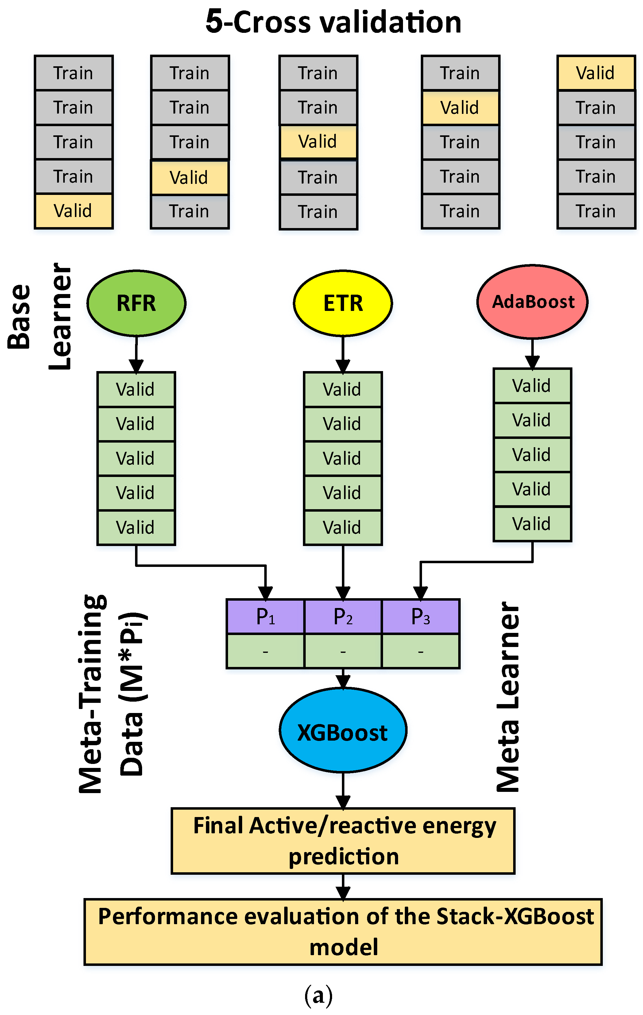
3.5. Stack-XGBoost

Stacked generalization, commonly referred to as stacking, represents an extra ensemble learning methodology devised by Wolpert [49], which has garnered substantial traction across diverse domains since its inception. Stacking orchestrates the consolidation of outcomes from various models such as random forest and AdaBoost, among others, with the objective of training a novel meta-learner for final predictions. The underpinning framework of stacking is structured on a dual-tiered algorithmic architecture. The initial tier comprises an array of algorithms denoted as base learners, while the succeeding tier encompasses a meta-learner recognized as a stacking algorithm. The first-tier learners frequently encompass distinct base models; however, stack ensembles can also be constructed utilizing identical base learner models [50]. These first-tier learners are honed to forecast outcomes employing the original dataset. Subsequently, the predictions from each base learner are aggregated to form a novel dataset, encompassing forecasts generated by these foundational learners. The second-tier meta-learner then employs this amalgamated dataset to generate the ultimate prediction. The primary role of the meta-learner is to rectify errors stemming from the base models by fine-tuning the ultimate prediction output. It is important to note that multiple stacking layers are feasible, with each level’s prediction serving as an input for the ensuing one. Stacking emerges as one of the best-sophisticated ensembles learning techniques. It adeptly mitigates both bias and variance, effectively averting overfitting concerns.

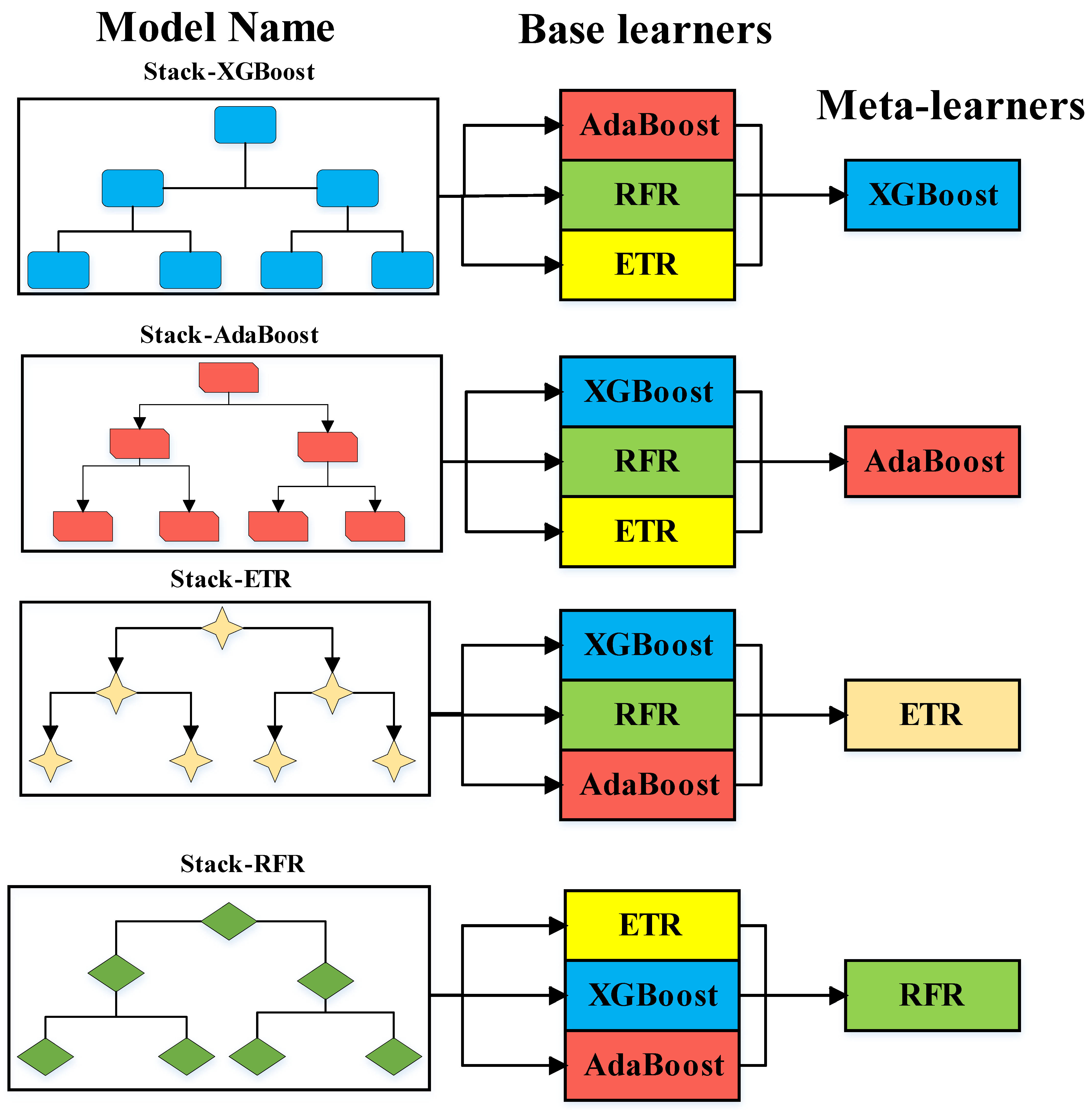
This study emphasizes the capabilities inherent in stacked ML models, exemplified through a flexible implementation that embodies an ensemble architecture. The core objective of this stacking approach resides in the quest to discern the optimum amalgamation of models catering to active and reactive energy forecasting. As a result, four distinct stack models are instantiated, as depicted in Figure 7 The base learner constitutes the distinct learning algorithm employed to generate predictions from the dataset. On the other hand, the meta-learner undertakes the task of amalgamating the predictions derived from the base learners to formulate a conclusive prediction. In addition, the meta-learner’s role involves acquiring the knowledge of effectively fusing the outputs of the base learners, thereby optimizing the comprehensive predictive performance.

The preparation of the training dataset for the meta-model involves a five-fold cross-validation of the base models, with the out-of-fold predictions serving as the foundation for this dataset. The comprehensive process underlying the proposed Stack-XGBoost model is graphically depicted in Figure 8, whereas the sequential steps involved in creating and evaluating the proposed model are illustrated in Figure 9. Finally, the sequential stages of the developed Stack-XGBoost model unfold as follows:

Stage 1: The first stage is selecting the dataset and checking on its variables; the selected dataset is for the small-scale steel industry, and it includes active energy consumption, lag/lead reactive energy consumption, lag/lead power factor, CO₂, time and date, number of seconds from midnight, load type, week status, and the day of the week.

Stage 2: The subsequent phase involves data preprocessing and scaling. The gathered data is averaged and scaled in accordance with the chosen forecasting horizon, as outlined in Section 2.1. Subsequently, the data is partitioned into training and testing sets, maintaining an 80:20 ratio.

Stage 3: The initial tier of the Stack-XGBoost framework comprises the foundational models (XGBoost, AdaBoost, and RFR). These foundational models conduct predictions for the active/reactive energy consumption through a five-fold cross-validation approach. The default configuration settings of the XGBoost algorithm as implemented in the scikit-learn (sklearn) library have been employed in this study.

Stage 4: The second tier of the Stack-XGBoost framework comprises a Meta-Regressor (XGBoost), which accepts the aggregated forecasts of the base models (M*Pi) as input to generate the ultimate prediction. The processing time is determined through parallel computational techniques, involving the computation of processing time at the initial stage, specifically the maximum time within the first layer, as well as the processing time required for the meta-learner within the second layer.

Stage 5: Finally, the evaluation of the developed Stack-XGBoost method is conducted utilizing the performance indices outlined in Section 2.3.

4. Results and Discussion

Within this work, a total of eight regression-based models (namely, RFR, XGBoost, AdaBoost, ETR, Stack-ETR, Stack-XGBoost, Stack-AdaBoost, and Stack-RFR) were systematically trained to predict active/reactive energy, as delineated in the Methodology section. The performance of each model was rigorously assessed using the dedicated testing dataset. Following individual training using distinct performance metrics such as RMSE, MAE, MSE, and R², the evaluation was conducted. Finally, diverse active/reactive forecasting scenarios were taken into account, encompassing 15 min, 30 min, and one hour ahead.

4.1. Scenario 1: Active/Reactive Energy Forecast (One Hour Ahead)

This first scenario will meticulously examine the outcomes derived from the forecasting results for active/reactive energy, specifically focusing on one hour ahead. This assertion is substantiated by the model’s accomplishment of the lowest RMSE, MAE, and MSE values for active energy, along with lagging and leading reactive energy. These commendable findings of scenario 1 are comprehensively outlined in the accompanying

Table 2. The forecasting results for the proposed Stack-XGBoost in scenario 1 compared to other models for one hour ahead.

Models	Metrics	RMSE	MAE	MSE	R2
	Energy
RFR	$E_{P }$	1.76	1.07	3.1	0.9969
	$E_{+Q }$	0.65	0.24	0.42	0.9904
	$E_{-Q }$	0.83	0.41	0.68	0.9969
XGBoost	$E_{P }$	1.72	1.03	2.95	0.997
	$E_{+Q }$	0.62	0.25	0.39	0.9912
	$E_{-Q }$	0.75	0.38	0.57	0.9974
AdaBoost	$E_{P }$	1.88	1.18	3.55	0.9965
	$E_{+Q }$	0.7	0.28	0.48	0.989
	$E_{-Q }$	1.13	0.71	1.28	0.9942
ETR	$E_{P }$	1.74	0.95	3.02	0.997
	$E_{+Q }$	0.65	0.23	0.43	0.9903
	$E_{-Q }$	0.81	0.37	0.66	0.997
Stack-ETR	$E_{P }$	1.44	0.87	2.07	0.9979
	$E_{+Q }$	0.62	0.2	0.38	0.9914
	$E_{-Q }$	0.67	0.31	0.44	0.998
Stack-XGBoost	$E_{P }$	1.38	0.8	1.9	0.9981
	$E_{+Q }$	0.61	0.2	0.38	0.9915
	$E_{-Q }$	0.65	0.3	0.43	0.9981
Stack-AdaBoost	$E_{P }$	1.54	0.89	2.38	0.9976
	$E_{+Q }$	0.62	0.22	0.39	0.9912
	$E_{-Q }$	0.69	0.31	0.48	0.9978
Stack-RFR	$E_{P }$	1.62	0.93	2.62	0.9974
	$E_{+Q }$	0.62	0.21	0.39	0.9913
	$E_{-Q }$	0.7	0.31	0.5	0.9978

. In general, it can be observed from the results that the Stack-XGBoost model, as proposed in this scenario, showcased exceptional performance by attaining the most accurate outcomes with less error.

To exemplify, the Stack-XGBoost model demonstrated a remarkable RMSE value of 1.38 for active energy, 0.61 for lead reactive energy, and 0.65 for lagging reactive energy. This outperformed the Stack-ETR and Stack-AdaBoost models, which achieved values of 1.62, 0.62, 0.7, and 1.54, 0.62, 0.69, respectively. Furthermore, the proposed Stack-XGBoost exhibited the lowest MAE and MSE, registering values of 0.8 and 1.9 for active energy, surpassing other models like Stack-ETR and Stack-AdaBoost, which yielded MAE and MSE values of 0.87, 2.07, and 0.22, 0.39, respectively. In the realm of lead reactive energy, the proposed model achieved an impressive MAE value of 0.2 and a MSE value of 0.38.

In contrast, the AdaBoost and RFR models exhibited subpar performance, showcasing the highest RMSE values of 1.88 and 1.76, respectively. The outcomes for the leading and lagging reactive energy models mirror this pattern. To provide a deeper understanding of the forecasting outcomes, Figure 10 visually presents the forecasted values alongside the actual values for various models. The depiction reveals that the models achieved reasonable approximations for active, lead reactive, and lag reactive energy, with the lines closely following the path of the actual data. However, concerning active energy, the model’s predictions sometimes diverge from the actual values, as indicated by the discrepancies between the lines and the actual data. This can be attributed to the higher RMSE values for specific models compared to others, a trend further evident in Figure 10a. For Figure 10b,c, the majority of lines correspond well with the actual values, reflecting the high R² values for most of the proposed models. Overall, it can be seen that the stacked models perform better than the single model according to the performance mercies.

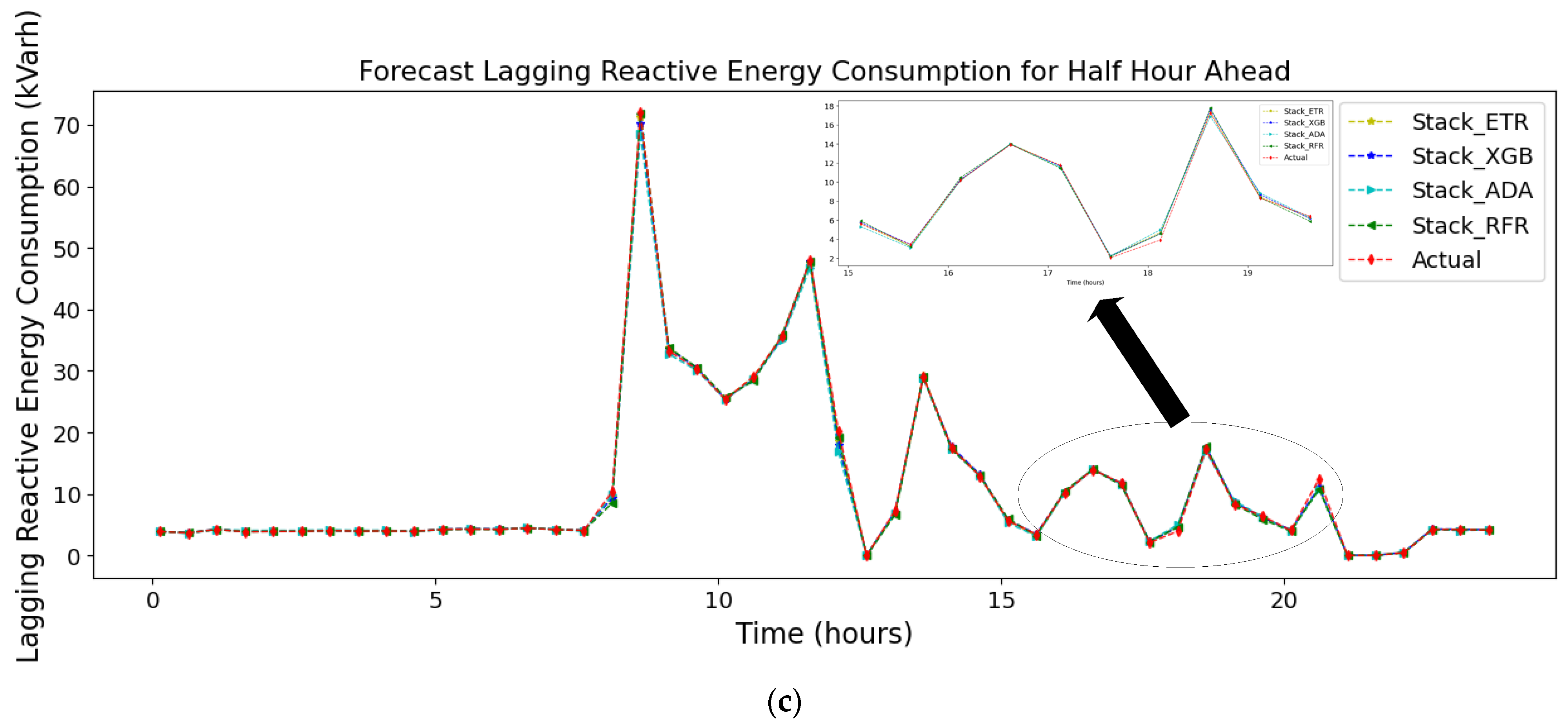
4.2. Scenario 2: Active/Reactive Energy Forecast (30 Min Ahead)

In the second scenario, the outcomes of the forecasting results for the active/reactive energy for a half hour ahead is presented. Overall, it is evident that the Stack-XGBoost model developed in this work demonstrated superior performance by achieving the most favorable results, as evidenced by the attainment of the lowest RMSE, MAE, and MSE values for the active energy and the lagging/leading reactive energy, as presented in the accompanying

Table 3. The forecasting results for the proposed Stack-XGBoost in scenario 2 compared to other models for 30 min ahead.

Models	Metrics	RMSE	MAE	MSE	R2
	Energy
RFR	$E_{P }$	1.89	1.11	3.57	0.9967
	$E_{+Q }$	0.49	0.18	0.24	0.995
	$E_{-Q }$	0.62	0.26	0.38	0.9985
XGBoost	$E_{P }$	1.47	0.71	2.16	0.998
	$E_{+Q }$	0.49	0.19	0.24	0.9951
	$E_{-Q }$	0.58	0.29	0.34	0.9987
AdaBoost	$E_{P }$	1.62	0.8	2.61	0.9976
	$E_{+Q }$	0.58	0.23	0.34	0.993
	$E_{-Q }$	0.7	0.31	0.49	0.9981
ETR	$E_{P }$	1.51	0.75	2.29	0.9979
	$E_{+Q }$	0.46	0.15	0.21	0.9957
	$E_{-Q }$	0.62	0.25	0.38	0.9985
Stack-ETR	$E_{P }$	1.31	0.75	1.71	0.9984
	$E_{+Q }$	0.41	0.18	0.18	0.9963
	$E_{-Q }$	0.49	0.21	0.24	0.9991
Stack-XGB	$E_{P }$	1.16	0.62	1.35	0.9987
	$E_{+Q }$	0.41	0.17	0.18	0.9962
	$E_{-Q }$	0.48	0.20	0.22	0.9991
Stack-AdaBoost	$E_{P }$	1.28	0.67	1.63	0.9985
	$E_{+Q }$	0.44	0.19	0.19	0.9961
	$E_{-Q }$	0.49	0.21	0.24	0.9991
Stack-RFR	$E_{P }$	1.36	0.7	1.84	0.9983
	$E_{+Q }$	0.43	0.18	0.19	0.9962
	$E_{-Q }$	0.49	0.21	0.23	0.9991

.

To illustrate, the Stack-XGBoost model achieved a RMSE value of 1.16, 0.41, and 0.48 for the active energy, lead reactive energy, and lag reactive energy, respectively, surpassing the Stack-ETR, Stack-RFR, and Stack-AdaBoost models, except for the $E_{+Q }$, where the Stack-ETR achieved the same results, and the models attained RMSE values for the $E_{P }$, $E_{+Q }$, $E_{-Q }$ of 1.31, 0.41, 0.49 for Stack-ETR, 1.36, 0.43, 0.49 for Stack-RFR, and 1.28, 0.44, 0.49 for Stack-AdaBoost, respectively. Further, the proposed Stack-XGBoost managed to obtain the lowest the MAE and MSE with a value of 0.62 and 1.35, respectively, for the active energy, surpassing the other models, such as Stack-ETR and Stack-AdaBoost which achieve a MAE and MSE value of 0.75, 1.71 and 0.67, 1.63, respectively. In the case of the lead reactive energy, the proposed model obtained a value of 0.17 for the MAE and 0.18 for the MSE, which is the lowest compared to the other proposed models.

On the contrary, the AdaBoost and RFR models exhibited poor performance, recording the highest $E_{P }$ RMSE values of 1.62 and 1.89, respectively. The other results for the leading and lagging reactive energy follow the same pattern.

To give more insight into the forecasting results, Figure 11 shows the predicted values along with the real values for different models. It can be seen that the models approximately predicted the active, lead reactive, and lag reactive energy, where the lines most match the ground truth line. However, in the case of the active energy, it is obvious that the lines match the ground truth line. Still, sometimes it mismatches it, which can be interpreted by the higher RMSE values for some models compared to other models and can also be seen in Figure 11a. For Figure 11b,c, most the lines are matched with the actual value, which can be interpreted by the high R² values for most of the proposed models. It is worth noting that the Stack models perform better than the single models as shown in Table 3. Further, it can be observed that the RMSE, MAE, and MSE values are smaller in the 30 min ahead forecasting compared to the one hour ahead forecasting, which can be explained by using a greater number of samples to train the models, resulting in more accurate solutions.

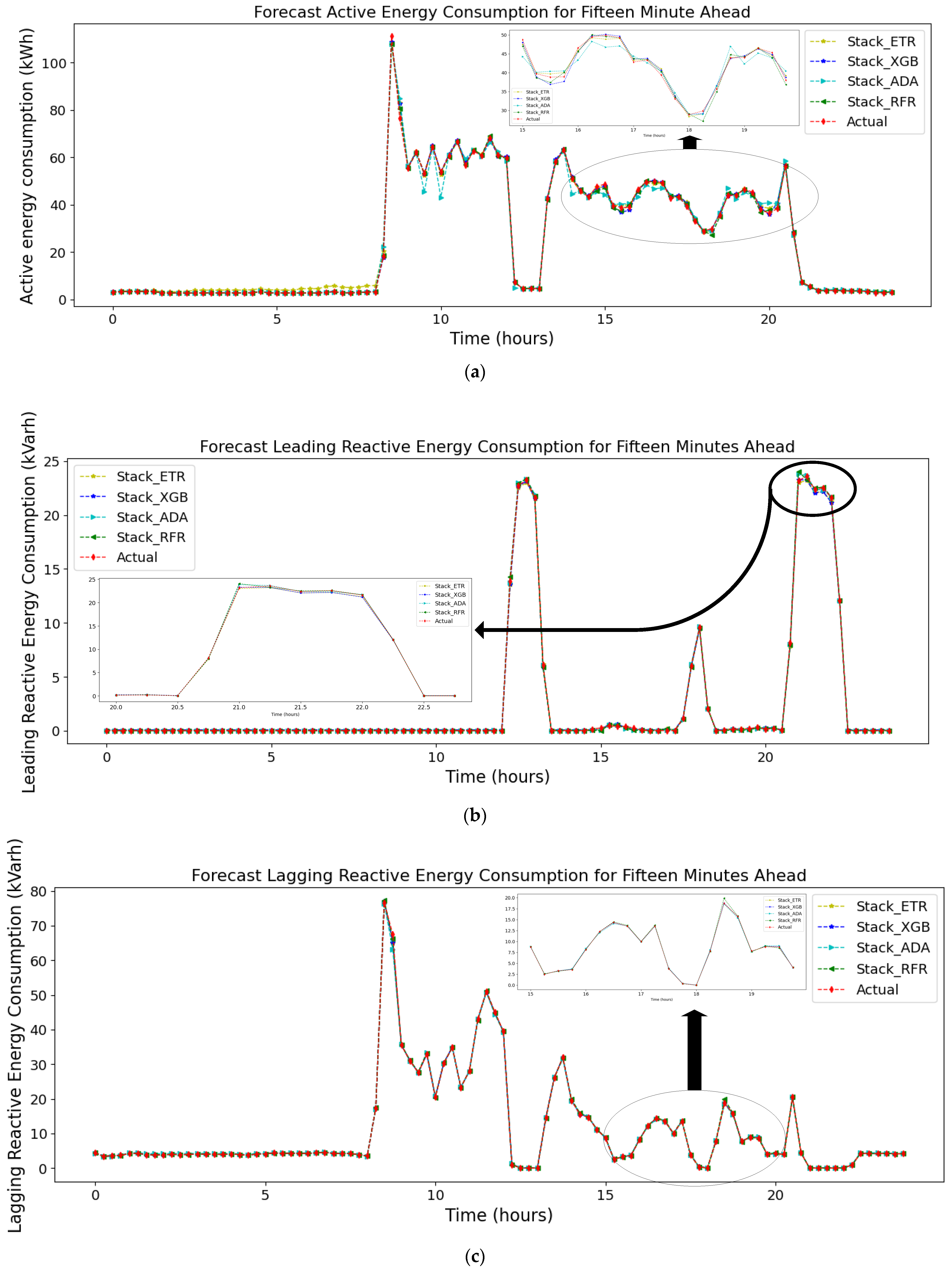
4.3. Scenario 3: Active/Reactive Energy Forecast (15 Min Ahead)

The final scenario will elaborate on the attained results of the forecasting for the active/reactive energy for the next 15 min. This is substantiated by the achievement of the lowest values for RMSE, MAE, and MSE in relation to the active energy and the lagging/leading reactive energy, as illustrated in

Table 4. The forecasting results for the proposed Stack-XGBoost in scenario 3 compared to other models for 15 min ahead.

Models	Metrics	RMSE	MAE	MSE	R2
	Energy
RFR	$E_{P }$	1.13	0.41	1.29	0.9989
	$E_{+Q }$	0.18	0.06	0.03	0.9994
	$E_{-Q }$	0.43	0.21	0.18	0.9993
XGBoost	$E_{P }$	0.97	0.44	0.94	0.9992
	$E_{+Q }$	0.18	0.06	0.03	0.9994
	$E_{-Q }$	0.41	0.21	0.16	0.9994
AdaBoost	$E_{P }$	1.23	0.54	1.52	0.9987
	$E_{+Q }$	0.33	0.13	0.11	0.9979
	$E_{-Q }$	0.74	0.48	0.55	0.998
ETR	$E_{P }$	0.99	0.42	0.97	0.9991
	$E_{+Q }$	0.16	0.1	0.02	0.9995
	$E_{-Q }$	0.27	0.09	0.07	0.9997
Stack-ETR	$E_{P }$	0.9	0.48	0.81	0.9993
	$E_{+Q }$	0.16	0.1	0.02	0.9995
	$E_{-Q }$	0.27	0.09	0.07	0.9997
Stack-XGB	$E_{P }$	0.69	0.35	0.47	0.9996
	$E_{+Q }$	0.13	0.05	0.02	0.9997
	$E_{-Q }$	0.22	0.09	0.05	0.9998
Stack-AdaBoost	$E_{P }$	0.81	0.36	0.66	0.9994
	$E_{+Q }$	0.17	0.11	0.03	0.9994
	$E_{-Q }$	0.26	0.09	0.07	0.9998
Stack-RFR	$E_{P }$	0.88	0.39	0.78	0.9993
	$E_{+Q }$	0.16	0.1	0.02	0.9995
	$E_{-Q }$	0.23	0.1	0.05	0.9998

for scenario 3. Overall, it can be seen that the Stack-XGBoost model, as proposed in this work, showcases exceptional performance by attaining the least error with high R².

To elucidate, the Stack-XGBoost model has achieved remarkable results, as evidenced by its RMSE values of 0.69, 0.13, and 0.22 for active energy consumption, leading reactive energy, and lagging reactive energy, respectively. These outcomes demonstrate its superiority over the Stack-ETR, Stack-RFR, and Stack-AdaBoost models, except for the cases of $E_{+Q }$ and $E_{-Q }$, where Stack-RFR achieved identical results. Specifically, the Stack-ETR, Stack-RFR, and Stack-AdaBoost models yielded RMSE values of 0.9, 0.16, and 0.27 for $E_{P }$; 0.88, 0.16, and 0.23 for $E_{+Q }$; and 0.81, 0.17, and 0.26 for $E_{-Q }$, respectively. Furthermore, the proposed Stack-XGBoost model outperformed its counterparts in terms of MAE and MSE, showcasing values of 0.35 and 0.47 for active energy consumption, surpassing Stack-AdaBoost and Stack-RFR, which displayed MAE and MSE values of 0.36, 0.66 and 0.41, 1.29, respectively. In the case of $E_{+Q }$, the proposed model achieved an MAE of 0.05 and an MSE of 0.02, emerging as the frontrunner among the proposed models. Moreover, for $E_{-Q }$, the proposed Stack-XGBoost model demonstrated the lowest MAE and MSE values, with figures of 0.09 and 0.05, respectively.

On the other hand, the AdaBoost and RFR models displayed subpar performance, registering the highest RMSE values for $E_{P }$ forecasting at 1.23 and 1.13, respectively. A similar trend was observed in the results for leading and lagging reactive energy forecasting. To provide deeper insights into the forecasting results, Figure 12 visually presents the predicted values juxtaposed with the actual values for the various models. Notably, the models exhibited satisfactory predictions for active, lead reactive, and lag reactive energy, with the plotted lines closely aligning with the ground truth line. The fluctuations observed in the graphs represent variations in both active and reactive energy consumption during the specified timeframe. It is evident that energy consumption is not consistent throughout this period. Therefore, the fluctuations in consumption are contingent on the specific consumption levels at each juncture due to the dynamic behavior of steel companies’ active/reactive energy consumption. Hence, understanding this dynamic behavior is crucial for optimizing energy usage and improving the efficiency and sustainability of steel manufacturing processes.

Particularly noteworthy is the alignment of the proposed model’s predictions with the ground truth line for active energy, corroborated by high R² values (0.9996 for $E_{P }$, 0.9997 for $E_{+Q }$, and 0.9998 for $E_{-Q }$) indicating an excellent fit to the dataset, as depicted in Figure 12a–c. In Figure 12b,c, a substantial portion of the lines closely corresponds with the actual values, a correlation supported by high R² values across most of the proposed models. It is worth highlighting that the Stack models showcased superior performance in comparison to the single models, a trend also substantiated in Table 4. Furthermore, it is apparent that the 15 min ahead forecasting exhibited smaller RMSE, MAE, and MSE values compared to the 30 min and one hour ahead forecasting. This can be attributed to the increased number of training samples, enabling the models to generate more accurate predictions by leveraging a larger dataset.

In conclusion, Figure 13 aptly demonstrates the convergence of the forecasted outcomes generated by the models with the actual values, offering a multifaceted view. Observing the figure, it becomes evident that the proposed Stack-XGBoost model outperforms the other models, exhibiting an almost indistinguishable resemblance to the actual values. Subsequently, the Stack-RFR model also exhibits commendable performance by consistently achieving the lowest RMSE values for both models. In contrast, models like XGBoost exhibit suboptimal performance, as evidenced by instances where the plotted points deviate from the reference line. This substantiates the assertion that the stacked models exhibit superior predictive capability compared to individual models. This pattern is consistent across all scenarios.

4.4. Sensitivity Indices

Sensitivity analysis entails the assignment of a “sensitivity index” to every input of a model. Calculating these indices involves several methods, which are relatively straightforward when the model is mathematically well-defined. Nevertheless, in more intricate scenarios, deriving these sensitivity indexes presents challenges [51]. Statistical methodologies can be used to numerically ascertain these sensitivity indexes by changing the model’s inputs and assessing their influence on the model’s output. A substantial body of research has been dedicated to sensitivity analysis, as evident in numerous published works. Based on the existing literature, sensitivity analysis can be classified into three main techniques: screening, local, and global sensitivity. The subsequent sections aim to evaluate the ramifications of input variability on the output by recognizing the part of output change accredited to peculiar inputs or input sets. The domain of sensitivity assessment involves a multifaceted range of metrics designed to evaluate the sensitivity of a model [52]. Noteworthy among these sensitivity metrics are the Standardized Regression Coefficient (SRC) and Kendall’s tau coefficient (KTC). Subsequently, comprehensive elucidation of these indices is presented in the ensuing sections.

The SRC evaluates the strength of the relationship among an output variable Y and a specific input variable $X_i$ through the application of a LR model. The R² value of this linear model, known as the correlation coefficient, plays a pivotal role in determining the precision and reliability of the SRC [53]. The subsequent equation represents the mathematical formulation of the linear model (Equation (17)).

$$Y={\beta }_o+\sum _{i=1}^K{\beta }_i{X}_i$$

(17)

$$V(Y)=\sum _{i=1}^K{{\beta }_i}^{2}V(X_i)$$

(18)

$${SRC}_i=\frac{{{\beta }_i}^{2}V(X_i)}{V(Y)}$$

(19)

where the variables $X_i$ are assumed to be independent, the variance of Y is demonstrated in Equation (18), and the SRC sensitivity indicator of the variable $X_i$ can be determined by using Equation (19). Finally, ${{\beta }_i}^{2}V(X_i)$ indicates the influence of the variable $X_i$ in the variance of $Y$. Hence, the SRC index expresses the variance of Y effect from variable $X_i$.

Finally, the KTC calculates the numerical linkage among two calculated variables. It functions as a non-parametric hypothesis test for evaluating statistical interdependence, with the coefficient denoting rank correlation, where the rank correlation signifies the resemblance in data orderings when ranked based on every respective variable.

The Sensitivity Analysis Outcomes for the Developed Techniques

To commence the discourse, this section will primarily concentrate on dissecting the findings concerning the 15 min forecast horizon; analogous trends are observed in the case of the other proposed timeframes. The outcomes of the sensitivity assessment, employing various sensitivity matrices, have been tabulated in

Table 5. The results of the sensitivity indices for the proposed models using the 15 min ahead results.

The Sensitivity Metrics for the 15 min Ahead Resolution Results Applied on a Steel Industry Dataset
Model	Metrics	SRC	KTC
	Energy
RFR	$E_P$	0.9955	0.9655
	$E_{+Q}$	0.9597	0.9541
	$E_{-Q}$	0.996	0.978
XGBoost	$E_P$	0.9975	0.9751
	$E_{+Q}$	0.9558	0.9355
	$E_{-Q}$	0.9954	0.9728
AdaBoost	$E_P$	0.9965	0.9705
	$E_{+Q}$	0.9558	0.9355
	$E_{-Q}$	0.9955	0.9737
ETR	$E_P$	0.9957	0.9668
	$E_{+Q}$	0.9638	0.9638
	$E_{-Q}$	0.9955	0.9737
Stack-ETR	$E_P$	0.9927	0.9482
	$E_{+Q}$	0.9548	0.958
	$E_{-Q}$	0.9954	0.9735
Stack-XGB	$E_P$	0.9976	0.9765
	$E_{+Q}$	0.9802	0.9702
	$E_{-Q}$	0.9994	0.9927
Stack-AdaBoost	$E_P$	0.9947	0.964
	$E_{+Q}$	0.956	0.9398
	$E_{-Q}$	0.9938	0.9595
Stack-RFR	$E_P$	0.9961	0.9687
	$E_{+Q}$	0.972	0.9397
	$E_{-Q}$	0.9954	0.9746

. The SRC serves as a rank correlation metric, gauging the monotonic connection among two variables without assuming a direct interrelation. The SRC’s scale spans from −1 to 1, where −1 represents an impeccable negative monotonic relationship, 1 denotes an impeccable positive monotonic relationship, and 0 signifies the absence of any monotonic association. In this particular context, the SRC coefficients are calculated to be 0.9976, 0.9802, and 0.9994 for the $E_{P }$, $E_{+Q }$, and $E_{-Q }$, respectively. These calculated values underscore a robust positive monotonic link among the real and forecasted values, indicating that as one parameter decreases, the other parameter also tends to follow suit. Such findings elucidate the model’s commendable ability in accurately capturing and representing this interrelationship.

Concluding the examination of correlation measures, the KTC emerges as another rank-centric metric, contrasting the tally of concordant pairs against discordant pairs within the dataset. Analogous to the earlier coefficients, KTC spans from −1 to 1; here, −1 means a flawless negative association, 1 shows an impeccable positive association, and 0 suggests an absence of any discernible association. In the ongoing analysis, the KTC values attributed to the Stack-XGBoost model are computed as 0.9765 for $E_{P }$, 0.9702 for $E_{+Q }$, and 0.9927 for $E_{-Q }$. These values affirm a robust positive correlation between the ground truth and estimated values, thereby reinforcing the precision of the proposed model’s prognostications and its commendable performance. All three coefficients closely align with the model’s forecasting against the actual values. Thus, the coefficients’ proximity to 1 underscores the Stack-XGBoost model’s capacity for accurately predicting the targeted variable. Finally, the Stack models have shown robust performance in comparison to the other proposed models.

5. Conclusions

This work proposes a stacked ensemble methodology, denoted as Stack-XGBoost, for active/reactive energy consumption, leveraging three distinct ML methods, including ETR, AdaBoost, and RFR, as base learner models. Further, the incorporation of an extreme gradient boosting (XGBoost) algorithm as a meta-learner serves to amalgamate the predictions generated by the base models, enhancing the precision of the active/reactive energy consumption forecasting using real-time data for the steel industry. The proposed models were applied to a real-time dataset related to the small-scale steel industry and validated using different performance metrics, such as RMSE, MAE, MSE, and R². The results revealed that the Stack-XGBoost model showed the best results in terms of RMSE, MAE, and MSE as compared to the alternative proposed models. In addition, it simultaneously achieved the highest R² value among the evaluated models. Furthermore, a thorough sensitivity analysis was conducted, encompassing critical parameters such as the Standardized Regression Coefficient and Kendall’s tau coefficient. This in-depth evaluation underscored the model’s resilience in the face of input parameter variations, affirming its robustness and reliability. Finally, the endeavor of forecasting active/reactive energy within the industrial sector carries significant implications that span a wide range of advantages. These encompass preserving financial resources, enhancing energy efficiency, ensuring equipment protection, complying with regulatory requirements, maintaining grid stability, and fostering improvements in environmental sustainability.

This study’s limitation is underscored by its focus on a singular dataset (steel industry dataset) for validating the proposed approach, consequently constraining the applicability of the obtained insights to consumption patterns in diverse industries and varying temporal contexts. To mitigate this limitation, the forthcoming expansion of this research will entail subjecting the proposed methodology to testing across disparate datasets representing various industries and geographical regions. Moreover, the deployment of the model within an end-to-end system will be pursued, facilitating an assessment of its efficacy under diverse circumstances. This deployment strategy is poised to enable ongoing enhancements and refinements grounded in real-time data analysis. The following recommendations for advancing the forecasting of active/reactive energy consumption in industrial sectors are succinctly outlined as follows:

• The selection of Stack-XGBoost in this study was driven by its characteristics delineated in the previous work and the empirical evidence it showcased. Still, there remains untapped potential for further enhancement, particularly in light of the ongoing evolution of novel deep learning models.
• Incorporating hyperparameter optimization can significantly augment the model’s predictive capabilities and merits consideration for future refinement.
• Expanding the scope by integrating additional parameters that interrelate with the active/reactive energy aspects, such as weather conditions, holds promise. The utilization of feature selection techniques can play a pivotal role in identifying the most pertinent variables.
• The investigation of meta-heuristic techniques for active/reactive energy forecasting can be contemplated by employing them for the purpose of tuning the model parameters.
• Finally, a compelling avenue for exploration involves subjecting the proposed model to real-time analysis and assessing its performance and pragmatic utility within industrial energy management systems [54].