Abstract
In this paper, a three-dimensional (3D) numerical model based on the finite element method (FEM) is developed to determine the fluid flow and heat transfer phenomena in a real multi-tube downhole heat exchanger (DHE), designed ad hoc for the present application, considering natural convection inside a geothermal reservoir. The DHE has been effectively installed and tested on the island of Ischia, in southern Italy, and the measurements have been used to validate the model. In particular, the authors analyze experimentally and numerically the behavior of the DHE based on the outlet temperature of the working fluid, thermal power, overall heat transfer coefficient, and efficiency. Furthermore, the influence of the degree of salinity on the performance of the DHE has been studied, observing that it degrades with the increase in the degree of salinity. The results show that the DHE allows to exchange more than 40 kW with the ground, obtaining overall heat transfer coefficient values larger than 450 W/m2 K. At the degree of salinity of 180 ppt, a decrease in the efficiency of the DHE of more than 8% is observed.
1. Introduction
The world is aiming to develop sustainable solutions towards meeting the domestic needs of the energy production and transportation sector, specifically to reduce greenhouse gas emissions and protect the environment [1]. The European Union has made increasing the use of renewable energy resources a high priority. Renewable energies accounted for 17.5% of the EU’s total energy consumption reported by Eurostat in 2017 [2]. The European Union has revised its target to achieve a share of at least 40% to 45% renewables in total energy consumption by the year 2030 [3]. Wide growth has been observed in solar-based and wind-based energy production, which accounts for about 17.5% and 7% of total renewable energy power plants worldwide [4]. Unfortunately, both these technologies are highly dependent upon weather conditions [5,6], and major fluctuations in electricity production have been observed, making them vulnerable to the conditions in a given geographical location on hourly, monthly, and seasonal bases [7].
Among the renewable energy sources, geothermal energy and biomass can provide more flexibility and enable continuous operation in electricity production [6,8]. To exploit geothermal energy in an effective way, heat exchangers are of the utmost importance. Heat exchangers are widely used for heating and cooling processes, including in industrial and agricultural applications (e.g., in greenhouses and aquaculture facilities), crop drying, food-processing dehydration, and water heating [9,10,11,12]. Heat exchangers can be installed underground, both horizontally and vertically. The vertical ones are typically better, especially when a high heat exchange capacity is required within a limited area [13]. In a vertical heat exchanger, several tubes, usually U-shaped, are arranged in a symmetrical circular pattern and buried in the ground at a certain depth. Heat is then extracted or conveyed to the ground by circulating a fluid (usually water) in the pipes in a closed circuit. The hole is usually filled with earth, mortar, or geothermal fluids [14,15].
A downhole heat exchanger (DHE) consists of several tubes, extracting heat from the geothermal reservoir via the circulation of a working fluid inside the tubes. It does not extract any geothermal fluid from the aquifer [16,17]; therefore, it does not require an extra well for the re-injection of geothermal fluid. Compared to other geothermal systems like ground-coupled heat pump (GCHP) systems, the DHE geothermal system has lower installation costs and higher availability [18].
Several studies have been conducted on GCHP systems to obtain higher efficiencies. Different analytical models have been developed, like 1D-line [19], helical-line [20], ring-coil [21] models, and for different shapes, like spiral [22], cylindrical heat source [23], and coaxial [24,25] models, for the optimization of the design of heat exchangers. The influences of different parameters, like working fluid flow rate, ground water flow, and backfill material thermal properties, for GCHP have also been studied [26,27]. Some studies have analyzed the installation costs and production performance of ground heat exchangers in GCHP systems [28,29].
As concerns DHEs, Carotenuto et al.’s [30] experimental studies verified the limitations of heat extraction with respect to DHEs. Carotenuto et al. [31,32] developed a lumped parameter model to study the heat and mass transfer between a geothermal well and a natural convection promoter. Galgaro et al. [33] employed the finite element method to conduct numerical simulations of mass and heat transfer inside porous media for a DHE array. A study on natural convection in a U-tube DHE under steady-state conditions was conducted by Gustafsson et al. [34]. Another steady-state model for a U-tube DHE was proposed by Lyu et al. [35]; it coupled a working fluid with a geothermal fluid inside a wellbore for the investigation of heat extraction. Carotenuto et al. [36] studied the saturated geothermal reservoir of a DHE system using 2D steady-state numerical simulations.
The previous studies on DHE systems provided significant insights into the heat transfer process, but almost all the models of DHE systems were either zero-dimensional (0D) or two-dimensional (2D) and mainly dealt with single- or double-tube U-shaped geometries, which do not effectively reproduce the behavior of real DHEs, which are made of multiple tubes. Moreover, there are few comprehensive studies on the influences of key factors on the heat extraction performance of DHEs. The performance of a DHE is also linked with the thermophysical properties of the working fluid in question; for example, properties like the viscosity, conductivity, and density of water vary from site to site and can change with time as well within the same location [37,38]. Even though the water being used is fresh water, the effects of the increase in the degree of salinity in water are also important for heat exchangers’ efficacy. Degree of salinity is the presence of salt in water, usually expressed in parts per thousand (ppt), i.e., grams of salt per kilogram of water. The increase in salinity can cause corrosion and degrades a heat exchanger’s tubes via fouling; therefore, the impact of these properties of water on heat transfer is relevant and cannot be ignored.
On the basis of the above analysis, in this paper, the authors experimentally and numerically analyzed, for the first time in the literature, a real DHE, designed and realized ad hoc for geothermal applications. The heat exchanger was inserted in a geothermal well on the island of Ischia in Southern Italy, and several experimental campaigns were undertaken to prove its efficacy and efficiency. Moreover, the authors developed a 3D numerical model able to reproduce the fluid flow and heat transfer inside the DHE and its interaction with the geothermal well. The numerical model was validated against the experimental data in terms of the outlet temperature of the working fluid, thermal power, the heat transfer coefficient, and efficiency. Furthermore, the effects on the efficiency of feeding the DHE with water characterized by different degrees of salinity were analyzed.
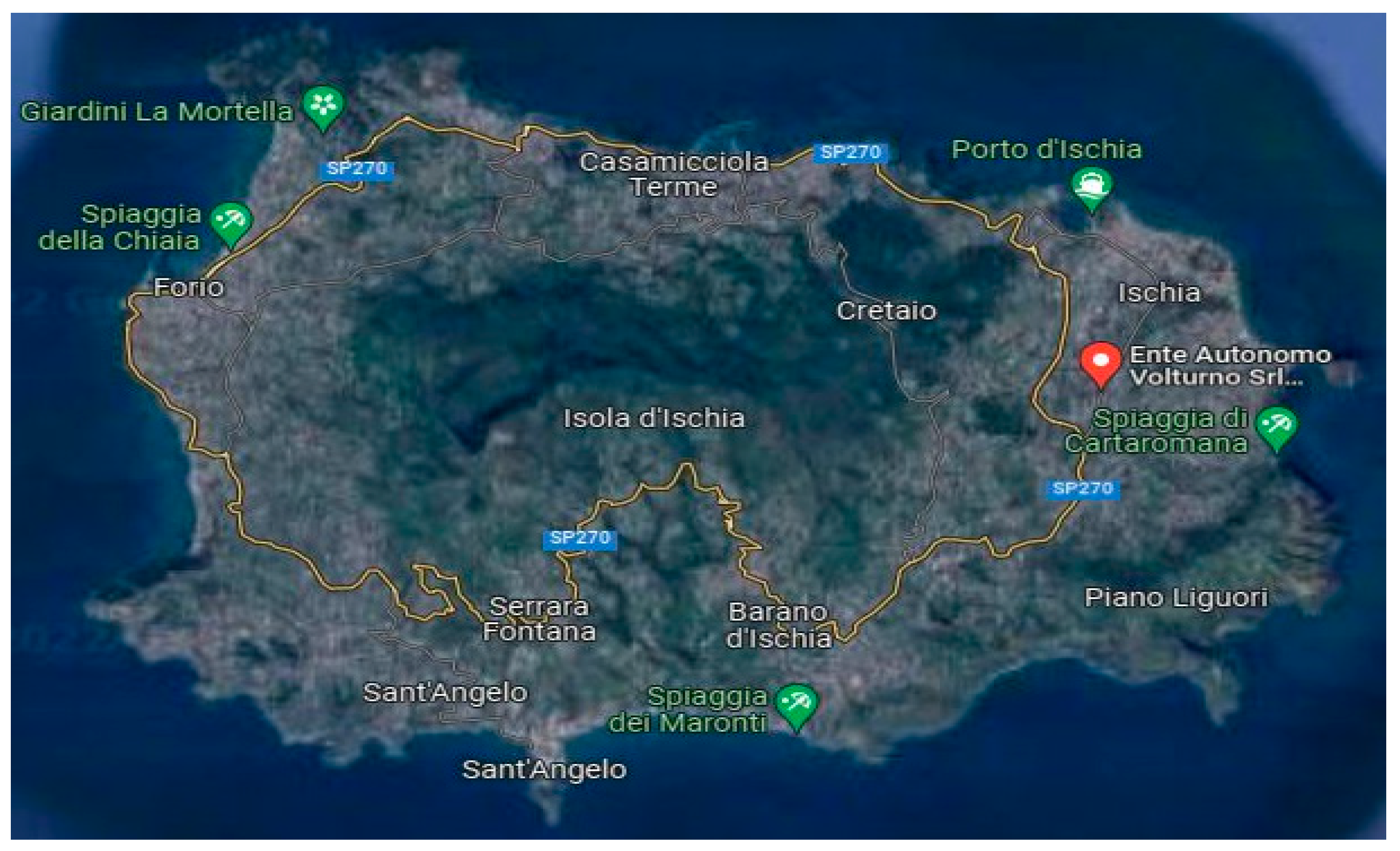
2. Experimental Setup
The experimental facilities have been installed and tested on the island of Ischia, in Southern Italy (Figure 1). The island of Ischia represents the emerged part of a large volcanic field that extends from Procida to the submarine volcanoes offshore of western Ischia.
Figure 1.
Island of Ischia in Southern Italy.
The experimental set-up mainly consists of: (i) the downhole heat exchanger (DHE), designed and realized ad hoc for geothermal applications (Figure 2); (ii) the aboveground heat dissipation system (dry cooler), employed to reproduce different working conditions of a user (Figure 3 right); (iii) the management and control apparatus, equipped with dedicated measurement and acquisition systems, pump, valves, safety components, and hydraulic connections (Figure 3 left).
Figure 2.
Downhole heat exchanger before installation in the geothermal well.
Figure 3.
Dry cooler (right) and management and control apparatus (left).
The heat transfer fluid receives thermal energy from the heat exchanger inserted in the geothermal well and transfers it to the dry cooler, which reproduces the terminals to be installed in an indoor environment of a real heating plant. Figure 4 describes the operation of the experimental device installed on the island of Ischia. The DHE inside the well is in contact with the aquifer, and heat exchange is favored by the installation of a filtering tube as a casing of the well in correspondence with the depth of the DHE (Figure 5).
Figure 4.
Illustration of the experimental device installed on the island of Ischia.
Figure 5.
Well casing (left) and filtering tube (right).
The construction of the well, which has a depth of about 100 m, has been carried out in several stages. The first phase involved the excavation of a reservoir having a diameter of 900 mm and a depth of about 25 m using the rotation technique. Subsequently, both rotation and percussion techniques were used, drilling with a diameter of 800 mm up to a depth of 45 m. The hole was lined with temporary lining tubes with a diameter of 800 mm and a thickness of 8 mm. The next phase involved the excavation of the well, with a diameter of 600 mm from the top to the bottom of the hole, through the use of the percussion technique. The final lining pipes were made of 316L stainless steel with an external diameter of 457 mm, a thickness of 6 mm, and an internal diameter of 445 mm.
The heat exchanger was 6 m long and composed of a single module. Internal baffles and steel tie rods were used to stiffen it further. It was made of AISI 316L stainless steel in order to ensure large resistance to corrosion due to the involvement of geothermal fluid. The heat exchanger consisted of 12 inlet flow pipes and 12 return pipes.
Since it is difficult to guarantee the perfect circularity of the section in the curvature, there is a head in the lower part of the heat exchanger that is similar to the upper one but lacks an internal septum to allow for the circulation of the heat transfer fluid. The upper and lower heads are depicted in Figure 6 and Figure 7, respectively.
Figure 6.
Upper head of DHE.
Figure 7.
Lower head of DHE.
The installation stage of the DHE inside the well is presented in Figure 8.
Figure 8.
Installation of the DHE inside the geothermal well.
The experimental set-up consisted of a dry cooler with variable thermal power from 5 kW to 90 kW and a maximum flow rate of 2.5 m3/h. It is, essentially, a finned-pack heat exchanger, typically used for cooling a fluid by means of air. In particular, the dry cooler chosen was equipped with (i) a heat exchanger employing copper pack and aluminum fins sized for temperatures up to 99 °C; (ii) EC brushless high-efficiency fans able to modulate up to 10% of the maximum air flow; and (iii) a painted AISI 9016 galvanized steel structure suitable for outdoor environments. The dry cooler was hydraulically connected to the management and control apparatus, which was connected to the DHE.
The circulation pump installed in the apparatus was designed via the calculation of pressure drops. The pump provides a pressure of at least 30 kPa in correspondence with a flow rate of 2.5 m3/h. The INT180 single-phase STRATOS 30/1-12 circulation pump with the IF-EXT OFF module (on/off and 0–10 v) was chosen; it can work with different flow rates of a fluid.
A dedicated management and control apparatus module was designed, including all the valves and components needed for the operation and management of the system, such as the acquisition system connected to all the sensors installed in the experimental facility. In particular, the module was equipped with an electromagnetic flow rate meter, pressure transducers, and Pt100 thermal probes for the measurement of inlet and outlet water temperatures, e.g., the data logger for the eight Pt100 temperature probes installed inside the well at different depths. These sensors were protected with a silicone cable and positioned from two meters above the heat exchanger to two meters below the heat exchanger. These sensors were extremely useful for monitoring the behavior of the aquifer when the heat exchanger was in operation and calculating the most adequate boundary conditions for the heat exchanger.
The thermal power exchanged by the DHE was calculated using two Pt100 temperature sensors on the flow and return pipes from the exchanger along with a flow rate meter.
It should be noted that Type A and Type B uncertainties were associated to the experimental measurements in order to calculate the combined uncertainty. Then, a coverage factor equal to two was used to obtain the expanded combined uncertainty, corresponding to a confidence level of 95.4%, based on Gauss distribution. Associating the uncertainties with the experimental data, the authors validated the numerical model by verifying that the numerical results fell within the uncertainty interval.
3. Description of Numerical Model
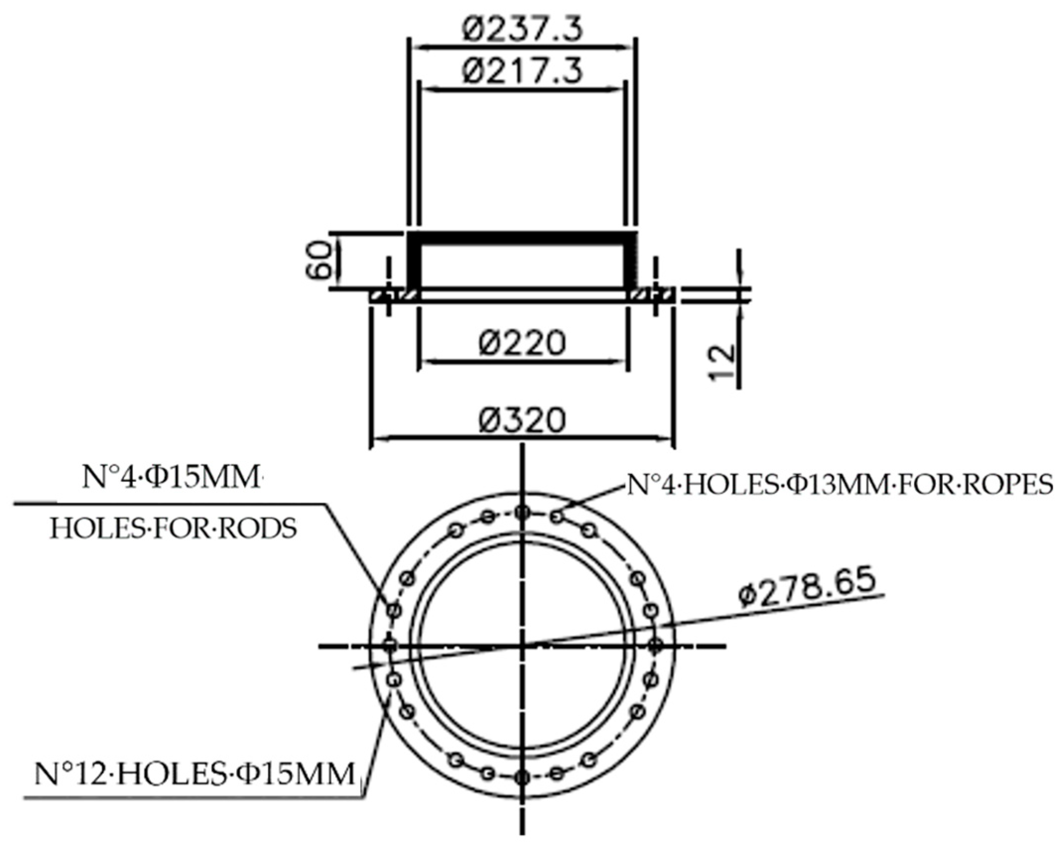
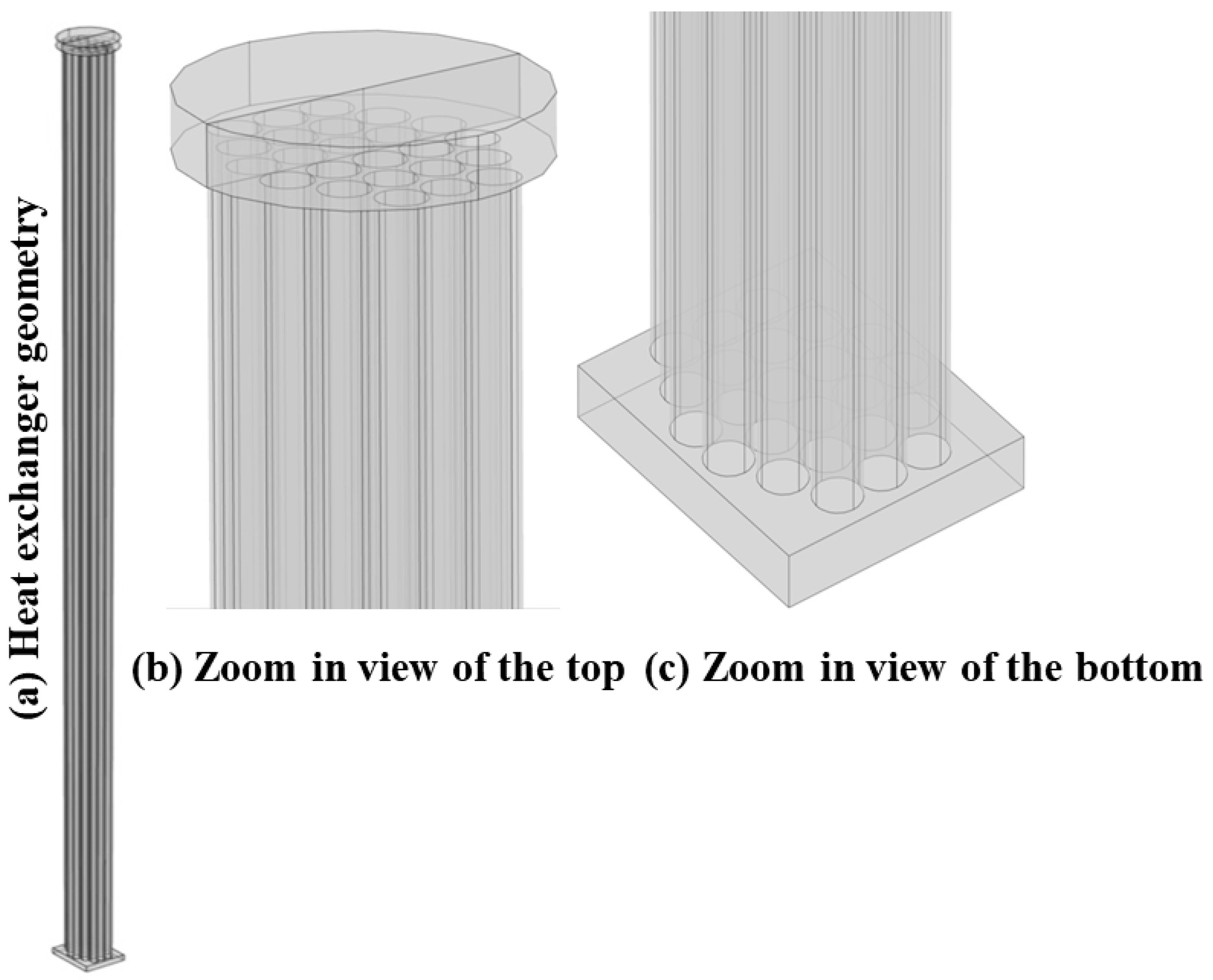
3.1. DHE Geometry
The geometry of the real DHE was reproduced using the commercial software Comsol Multiphysics version 5.5, as shown in Figure 9. The DHE consists of 24 tubes and a duct at the bottom of the heat exchanger. Water inflow occurs by means of 12 tubes, and another 12 tubes are used for outflow. The material used for the heat exchanger is AISI 316L steel. The main geometrical characteristics of the DHE are reported in Table 1.
Figure 9.
Geometry of the DHE.
Table 1.
Characteristics of the DHE.
3.2. Fluid Flow and Heat Transfer Model of the DHE
The Navier–Stokes Equation (1) was solved to reproduce the fluid flow inside the DHE.
The epsilon model was employed to reproduce the turbulent phenomena inside the DHE, and the energy conservation equation was implemented to determine heat transfer inside the DHE. The mathematical model used is as follows:
is the conductive heat flux, whereas the terms are related to the pressure changes and viscous dissipation in the fluid, respectively. As the flow is incompressible in this model, the terms and were neglected. The term (kg/m3) is the density of the working fluid, is the mass flow rate of the working fluid, and (W/m3) is the heat generation rate. Equation (2) is the kinetic energy transport equation, and the term yields the production of turbulent kinetic energy, which is expressed in Equation (4). Equation (3) represents the energy dissipation rate, and is turbulent viscosity given in Equation (5) to study the fluid flow. The equations were then coupled with the energy conservation equation, which is studied by using Equation (6) in the numerical model developed. Ce1 = 1.44, Ce2 = 1.92, Cµ = 0.09, σk = 1, and σε = 1.3 in the equations above are constants, and their values were taken from the experimental works of DC Wilcox [39].
3.3. Domain and Boundary Conditions
Water enters from the (top left half) inlet and exits from the other sides of the tubes, as shown in Figure 10. The DHE is immersed in the geothermal well, and it is directly in contact with the geothermal fluid; therefore, the convective heat flux boundary condition was applied at the external surfaces of the heat exchanger by means of Equation (7).
Figure 10.
Computational domain and boundary conditions.
The term represents the outer surface temperature of the heat exchanger, calculated using the numerical model, while represents the temperature of the geothermal fluid in the well, derived from the experimental data acquired during the measurement campaigns. In particular, was calculated as the average value of the temperature measurements inside the well, acquired by means of Pt100 sensors.
The heat transfer coefficient, , was calculated for the free convection of the geothermal fluid inside the well based on the correlations related to vertical cylinders [39]. In particular, the convective heat transfer coefficient, in Equation (8) is a function of the two dimensionless parameters, namely, the Rayleigh number (Equation (9)) and the Prandtl number (Equation (10)), which refers to natural convection, whereas in Equation (11) is the Grashof number.
The value of was calculated for each value of , as given in Table 2, and then used as a boundary condition for each case simulated by employing the numerical model. In particular, the model was used to reproduce eight different cases based on eight experimental values of the inlet temperature of the working fluid, well temperatures, and the convective heat transfer coefficient, as reported in Table 2.
Table 2.
Experimental data used to set the boundary conditions (the value of h was calculated by employing the measured data).
The properties of the geothermal fluid in terms of specific heat capacity, ; dynamic viscosity, ; thermal conductivity, ; and kinematic viscosity, , used in the above equations are reported in Table 3.
Table 3.
Values of properties employed in the model for the geothermal fluid.
The value of the Prandtl number is 7.01, while the values of the Reynolds, Grashof, and Rayleigh numbers are reported in Table 4 for the eight cases considered in the numerical simulations.
Table 4.
Values of non-dimensional numbers.
The effects of the degree of salinity of the working fluid have been studied by fixing the input data, particularly for the data of Case 2 (Table 2), in order to compare the obtained results for different salinity conditions with respect to fresh water. The properties of water for the different degrees of salinity employed in the numerical model are reported in Table 5.
Table 5.
Thermo-physical properties of water for different degrees of salinity.
3.4. Mesh Sensitivity Analysis
Due to the complex structure and large size of the geothermal heat exchanger, five tetrahedral meshes with 1.50, 1.55, 1.6, 2.2, and 4 million tetrahedral elements have been tested. The meshes have been chosen after a mesh sensitivity analysis, and Figure 11 shows a magnified image of the employed mesh near the bottom and top of the DHE. The computational grids also include three boundary layers to accurately capture the complex flow behavior near solid boundaries.
Figure 11.
Details of the computational grid at the bottom (left) and top (right) of the DHE.
The outlet temperature of the working fluid and computational time were calculated for the above five computational grids, as shown in Figure 12. According to the obtained numerical results, when the number of elements reached 1.6 million, a further increase in the number of elements led to a negligible variation in the outlet temperature. Moreover, the authors calculated the relative errors with respect to the experimental values of the outlet temperature for the five grid sizes. In particular, for 1.5, 1.55, 1.6, 2, and 4 million elements grids, the relative error was found to be 2.1%, 1.2%, 0.2%, 0.1%, and 0.09%, respectively. Therefore, the mesh with 1.6 million elements was chosen for all the simulations in order to save computational resources and ensure an adequate accuracy of the numerical results.
Figure 12.
Mesh sensitivity analysis and computational time for five grids.
3.5. Model Assumptions
In order to analyze the complex thermofluid dynamic phenomena inside the real 3D heat exchanger inserted in the geothermal well and, at the same time, to avoid using an excessive number of computational resources, the authors simplified the model by employing convective boundary conditions on the boundaries of the heat exchanger. Using this approach, the geothermal aquifer and the well were not reproduced in the 3D computational domain. However, in order to correctly reproduce the heat transfer performance of the DHE, the authors employed the on-site-acquired experimental data on the temperature of the geothermal fluid in the well to set the convective boundary condition reported in Equation (7).
A further development of the present model could take into account the reproduction of the well and aquifer in a 3D computational domain, with the consequent necessity of significantly more computational resources.
4. Results and Discussion
The computational model developed by the authors was used to simulate the eight cases reported in Table 2. The main performance parameters calculated in the present paper are the overall heat transfer coefficient, thermal power, the outlet temperature of the working fluid, and efficiency.
For the calculation of the overall heat transfer coefficient U, Equation (12) was used
where is the thermal power calculated from Equation (13) and A is the surface area of the heat exchanger
while is the logarithmic mean temperature, which is calculated using Equation (14) in the case of constant heat flux at the surface.
Furthermore
where is the mass flow rate of the working fluid, is the specific heat at constant pressure of the working fluid, is the inlet temperature of the working fluid, is the outlet temperature of the working fluid (which is calculated as the output of the 3D numerical model), and is the surface temperature of the heat exchanger.
Moreover, the efficiency of the DHE was calculated based on Equation (15), which was taken from reference [30]:
where is the mean temperature, that is, the average temperature between the inlet and outlet temperatures of the DHE, whereas and are the temperature at the top and bottom surfaces of the DHE, respectively, and they were measured using the temperature probes employed in correspondence with the top and bottom caps of the DHE.
Figure 13 shows that from the inlet-side tubes, the temperature of the heat exchanger starts to increase gradually; it then stabilizes when it reaches the mid height of the outlet side and remains this way until reaching the outlet.
Figure 13.
Surface temperature of the DHE.
4.1. Verification and Validation
The computational model was validated against the experimental data acquired on site for a real geothermal heat exchanger. For each case reported in Table 2, the values of the overall heat transfer coefficient, thermal power, outlet temperature, and efficiency have been calculated using the numerical model and compared with the corresponding experimental data. The experimental data used for the model’s validation are provided in Table 6.
Table 6.
Experimental data employed for model validation.
In the following sub-sections, the authors report the main results obtained using the numerical model and through comparison with the experimental data, together with the measurement uncertainties, that allowed them to both analyze the performance of the DHE and validate the numerical model.
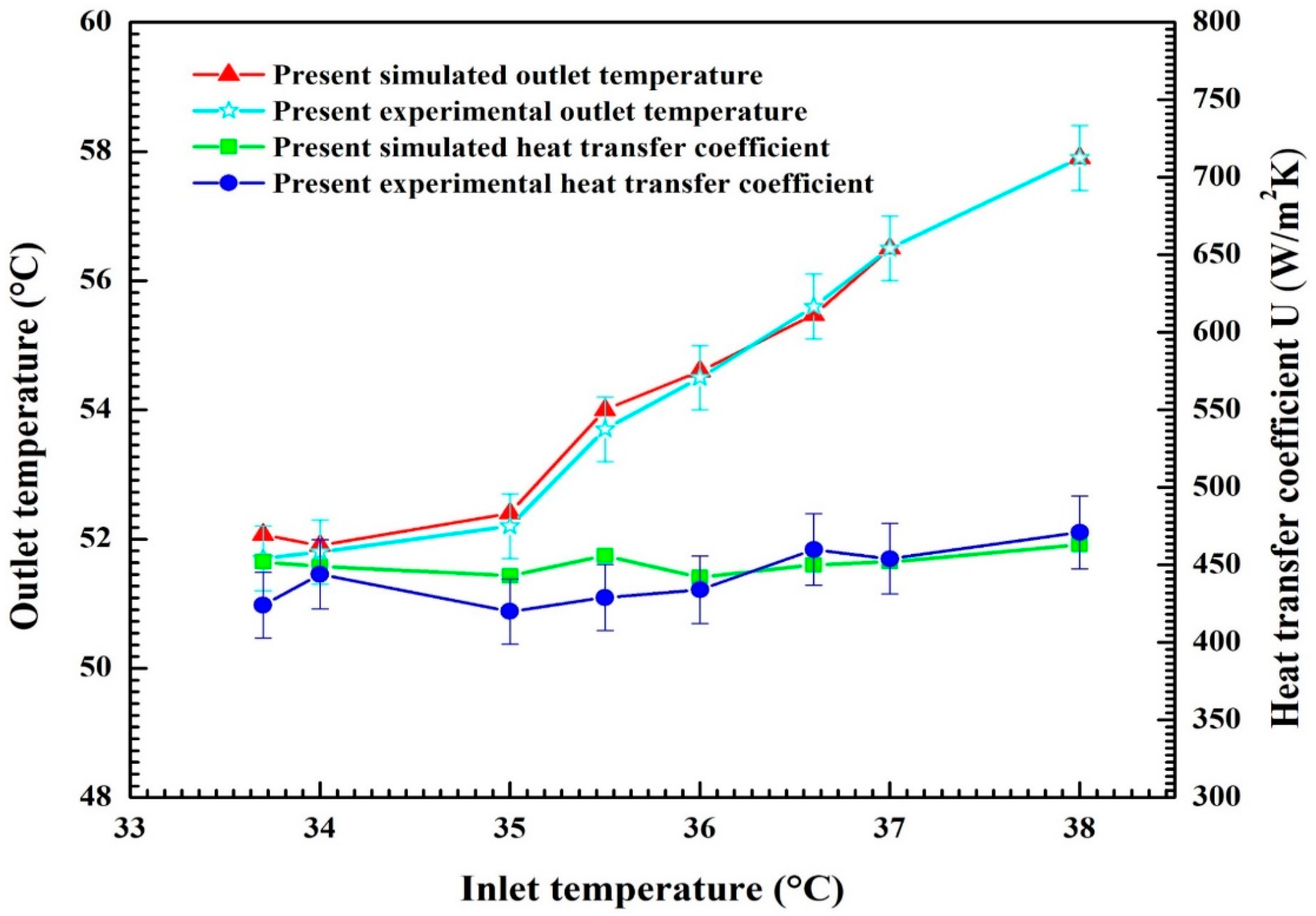
4.2. Outlet Temperature and Heat Transfer Coefficient
The authors calculated both the outlet temperature of the working fluid and the overall heat transfer coefficient and compared them with the corresponding experimental data for the eight cases reported in Table 2. Figure 14 shows both the calculated and measured values of these parameters together with the expanded combined uncertainty associated with each experimental point. It can be observed that the outlet temperature of the working fluid increases with the increase in the inlet temperature in a more pronounced manner than the overall heat transfer coefficient. In particular, the DHE is able to work with an overall heat transfer coefficient larger than 450 W/m2 K.
Figure 14.
Numerical and experimental results in terms of outlet temperature of working fluid and the overall heat transfer coefficient (U).
As shown in Figure 14, the numerical results are in excellent agreement with the experimental data. In particular, the numerical values fall within the uncertainty intervals for all but two of the experimental points.
4.3. Thermal Power and Efficiency
The increase in the inlet temperature of the working fluid leads to an increase in the output thermal power, , for cases 4 to 8 in Table 2, as shown in Figure 15. This phenomenon should be due to the more pronounced increase in the outlet temperature and to the increase in the heat transfer coefficient observed in the previous sub-section. In particular, the DHE is able to exchange more than 40 kW with the well, without causing freezing phenomena of the geothermal aquifer.
Figure 15.
Numerical and experimental results in terms of output thermal power and DHE efficiency.
However, a decrease in the efficiency of the DHE was observed, which should mainly be due to the decrease in Tbottom and the difference between and . In order to ensure greater efficiency, the inlet temperature should be kept as low as possible [40].
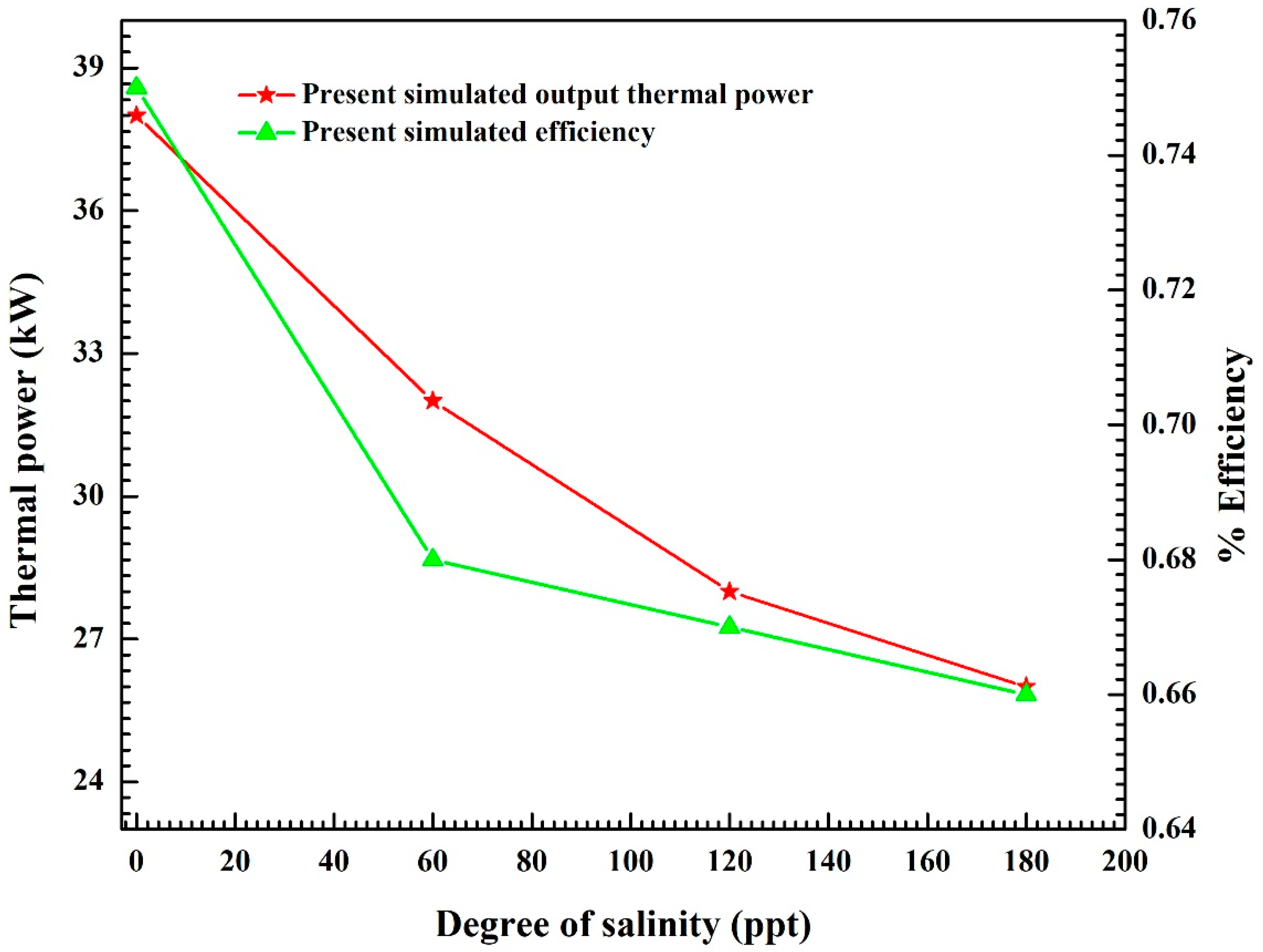
4.4. Effects of Degree of Salinity
The outlet temperature and heat transfer coefficient of the DHE, calculated using the present numerical model for different degrees of salinity of the working fluid, are reported in Figure 16. The thermos-physical properties of water for different degrees of salinity are reported in Table 5.
Figure 16.
Outlet temperature and heat transfer coefficient for different degrees of salinity of working fluid.
It can be observed that the outlet temperature decreases with the increase in the degree of salinity, and so does the heat transfer coefficient. When the molality is 180 ppt, decreases of more than 7% in outlet temperature and 50% in the heat transfer coefficient compared to those of fresh water are observed. Therefore, it is preferable to work with fresh water.
The output thermal power and efficiency for different degrees of salinity are reported in Figure 17. It is worth noting that the inlet temperature and boundary conditions used for each different value of salinity were kept constant (Case 2 of Table 2) to compare this performance with that of fresh water, i.e., m = 0. It can be observed that the increase in the salinity of water leads to a decrease in the overall performance of the heat exchanger in terms of, e.g., thermal power and efficiency. This occurs because when the degree of salinity of water increases, the amount of heat exchanged in the system decreases [41], leading to a decrease in the outlet temperature of the heat exchanger, and an overall decrease in system performance is observed.
Figure 17.
Effect of increase in degree of salinity on heat transfer coefficient and output thermal power of DHE.
A decrease greater than 8% in the efficiency of the DHE can be observed for a molality of 180 ppt, showing the importance of using fresh water or water with the lowest degree of salinity as a working fluid.
5. Conclusions
In this study, the authors have developed a three-dimensional thermo-fluid dynamic model to reproduce a real geothermal downhole heat exchanger (DHE). The experimental data acquired on-site on the island of Ischia, in southern Italy, have been employed to validate the numerical model.
The efficacy and efficiency of the geothermal heat exchanger have been analyzed. The k-epsilon model has been applied to reproduce the turbulence phenomena inside the DHE, while the thermal interaction between the DHE and the geothermal well has been studied by employing natural convective heat flux boundary condition, based on the experimental data. The validated model has allowed to calculate the outlet temperature of the working fluid, the overall heat transfer coefficient, the thermal power, and the efficiency. These data have been also obtained by means of the instruments available on the pilot plant installed on the island of Ischia, in order to compare the numerical and experimental results.
The results show that the DHE allows to exchange more than 40 kW with the geothermal well, without causing the phenomenon of ground freezing, obtaining overall heat transfer coefficient values larger than 450 W/m2 K. As expected, the increase in the convection mechanism allows to improve the DHE performance.
Moreover, the effects of the degree of salinity of water on the performance of the heat exchanger have been analyzed. An increase of the degree of salinity brings to a decrease of the outlet temperature and, consequently, of the efficiency of the DHE, i.e. more than 8% reduction when the degree of salinity is equal to 180 ppt.
The authors think that the present validated model could be used to further analyze real geothermal systems and to design its extension, based on the coupling with other heat exchangers.
Author Contributions
Conceptualization, M.A. and A.M.; Methodology, M.A.; Software, M.A.; Validation, M.A. and A.M.; Resources, V.G. and A.M.; Data curation, V.G.; Writing—original draft, M.A.; Writing—review & editing, A.M.; Supervision, A.M. All authors have read and agreed to the published version of the manuscript.
Funding
The authors gratefully acknowledge the financial support of project “REGGAE—Realizzazione di un pozzo Esplorativo e di un sistema di Geoscambio innovativo per l’utilizzo sostenibile di risorse Geotermiche A media Entalpia”, CUP B63D18000620007, POR Campania FESR 2014–2020 and of project “Development and optimization of innovative energy systems based on renewables”, DOT1341429-3, PON RI 2014-2020.
Data Availability Statement
Not applicable.
Conflicts of Interest
The authors declare no conflict of interest.
Nomenclature
| cp | specific heat capacity: J/kg K |
| Tinlet | inlet temperature, °C |
| Toutlet | outlet temperature, °C |
| Twell | temperature of the well, °C |
| m | molality, parts per thousand |
| U | overall heat transfer coefficient, W/m2 K |
| surface temperature of DHE, °C | |
| logarithmic mean temperature, °C | |
| L | characteristic length, m |
| thermal conductivity, W/m K | |
| q | heat flux, W/m2 |
| heat transfer, W | |
| convective heat transfer coefficient, W/m2 K | |
| Ra | Rayleigh number |
| Pr | Prandtl number |
| Gr | Grashof number |
| D | diameter of tube, m |
| mass flow rate, kg/s | |
| gravitational acceleration, m/s2 | |
| u | velocity, m/s |
| p | fluid pressure, Pa |
| I | identity matrix |
| ∇ | del operator |
| T | stress tensor |
| Greek symbols | |
| kinematic viscosity, m2/s | |
| thermal expansion coefficient, 1/K | |
| density, kg/m3 | |
| µ | dynamic viscosity, Ns/m2 |
| turbulent viscosity, Ns/m2 | |
| efficiency | |
| Acronyms | |
| HEX | heat exchanger |
| DHE | downhole heat exchanger |
| GCHP | ground coupled heat pump |
| FEM | finite element method |
References
- Sarkar, J.; Bhattacharyya, S. Application of Graphene and Graphene-Based Materials in Clean Energy-Related Devices Minghui. Arch. Thermodyn. 2012, 33, 23–40. [Google Scholar] [CrossRef]
- IRENA. Renewable Energy Statistics 2021. Stat. Focus-Eurostat 2021, 56, 460. [Google Scholar]
- EU Action to Address the Energy Crisis. Available online: https://commission.europa.eu/strategy-and-policy/priorities-2019-2024/european-green-deal/eu-action-address-energy-crisis_en (accessed on 27 January 2023).
- Ceglia, F.; Marrasso, E.; Roselli, C.; Sasso, M. Effect of Layout and Working Fluid on Heat Transfer of Polymeric Shell and Tube Heat Exchangers for Small Size Geothermal ORC via 1-D Numerical Analysis. Geothermics 2021, 95, 102118. [Google Scholar] [CrossRef]
- Watson, S. Quantifying the Variability of Wind Energy. Wiley Interdiscip. Rev. Energy Environ. 2014, 3, 330–342. [Google Scholar] [CrossRef]
- Bett, P.E.; Thornton, H.E. The Climatological Relationships between Wind and Solar Energy Supply in Britain. Renew. Energy 2016, 87, 96–110. [Google Scholar] [CrossRef]
- Calise, F.; D’Accadia, M.D.; MacAluso, A.; Piacentino, A.; Vanoli, L. Exergetic and Exergoeconomic Analysis of a Novel Hybrid Solar–Geothermal Polygeneration System Producing Energy and Water. Energy Convers. Manag. 2016, 115, 200–220. [Google Scholar] [CrossRef]
- Crainz, M.; Curto, D.; Franzitta, V.; Longo, S.; Montana, F.; Musca, R.; Sanseverino, E.R.; Telaretti, E. Flexibility Services to Minimize the Electricity Production from Fossil Fuels. A Case Study in a Mediterranean Small Island. Energies 2019, 12, 3492. [Google Scholar] [CrossRef]
- Yildirim, N.; Parmanto, S.; Akkurt, G.G. Thermodynamic Assessment of Downhole Heat Exchangers for Geothermal Power Generation. Renew. Energy 2019, 141, 1080–1091. [Google Scholar] [CrossRef]
- van der Zwaan, B.; Dalla Longa, F. Integrated Assessment Projections for Global Geothermal Energy Use. Geothermics 2019, 82, 203–211. [Google Scholar] [CrossRef]
- Martirosyan, A.V.; Martirosyan, K.V.; Grudyaeva, E.K.; Chernyshev, A.B. Calculation of the Temperature Maximum Value Access Time at the Observation Point. In Proceedings of the 2021 IEEE Conference of Russian Young Researchers in Electrical and Electronic Engineering, ElConRus 2021, Moscow, Russia, 26 January 2021; Institute of Electrical and Electronics Engineers Inc.: Piscataway, NJ, USA, 2021; pp. 1014–1018. [Google Scholar]
- Ilyushin, Y.; Golovina, E. Stability of Temperature Field of The Distributed Control System. ARPN J. Eng. Appl. Sci. 2020, 15, 664–668. [Google Scholar]
- Application of Ground Heat Exchangers|Encyclopedia MDPI. Available online: https://encyclopedia.pub/entry/10048 (accessed on 14 July 2022).
- Pouloupatis, P.D.; Florides, G.; Tassou, S. Measurements of Ground Temperatures in Cyprus for Ground Thermal Applications. Renew. Energy 2011, 36, 804–814. [Google Scholar] [CrossRef]
- Zeng, H.; Diao, N.; Fang, Z. Heat Transfer Analysis of Boreholes in Vertical Ground Heat Exchangers. Int. J. Heat Mass. Transf. 2003, 46, 4467–4481. [Google Scholar] [CrossRef]
- Luo, Y.; Guo, H.; Meggers, F.; Zhang, L. Deep Coaxial Borehole Heat Exchanger: Analytical Modeling and Thermal Analysis. Energy 2019, 185, 1298–1313. [Google Scholar] [CrossRef]
- Lund, J.W. The Use of Downhole Heat Exchangers. Geothermics 2003, 32, 535–543. [Google Scholar] [CrossRef]
- Aresti, L.; Christodoulides, P.; Florides, G. A Review of the Design Aspects of Ground Heat Exchangers. Renew. Sustain. Energy Rev. 2018, 92, 757–773. [Google Scholar] [CrossRef]
- Zeng, H.Y.; Diao, N.R.; Fang, Z.H. A Finite Line-Source Model for Boreholes in Geothermal Heat Exchangers. Heat Trans. Asian Res. 2002, 31, 558–567. [Google Scholar] [CrossRef]
- Li, M.; Lai, A.C.K. New Temperature Response Functions (G Functions) for Pile and Borehole Ground Heat Exchangers Based on Composite-Medium Line-Source Theory. Energy 2012, 38, 255–263. [Google Scholar] [CrossRef]
- Cui, P.; Li, X.; Man, Y.; Fang, Z. Heat Transfer Analysis of Pile Geothermal Heat Exchangers with Spiral Coils. Appl. Energy 2011, 88, 4113–4119. [Google Scholar] [CrossRef]
- Leroy, A.; Bernier, M. Development of a Novel Spiral Coil Ground Heat Exchanger Model Considering Axial Effects. Appl. Therm. Eng. 2015, 84, 409–419. [Google Scholar] [CrossRef]
- Man, Y.; Yang, H.; Diao, N.; Liu, J.; Fang, Z. A New Model and Analytical Solutions for Borehole and Pile Ground Heat Exchangers. Int. J. Heat Mass. Transf. 2010, 53, 2593–2601. [Google Scholar] [CrossRef]
- Morchio, S.; Fossa, M. Thermal Modeling of Deep Borehole Heat Exchangers for Geothermal Applications in Densely Populated Urban Areas. Therm. Sci. Eng. Prog. 2019, 13, 100363. [Google Scholar] [CrossRef]
- Akhmadullin, I.; Kartushinsky, A. CFD Simulation of Bubbly Flow in a Long Coaxial Heat Exchanger. Therm. Sci. Eng. Prog. 2021, 25, 100991. [Google Scholar] [CrossRef]
- Al-Zyoud, S.; Rühaak, W.; Sass, I. Dynamic Numerical Modeling of the Usage of Groundwater for Cooling in North East Jordan –A Geothermal Case Study. Renew. Energy 2014, 62, 63–72. [Google Scholar] [CrossRef]
- Han, C.; Yu, X. Sensitivity Analysis of a Vertical Geothermal Heat Pump System. Appl. Energy 2016, 170, 148–160. [Google Scholar] [CrossRef]
- Go, G.H.; Lee, S.R.; Nikhil, N.V.; Yoon, S. A New Performance Evaluation Algorithm for Horizontal GCHPs (Ground Coupled Heat Pump Systems) That Considers Rainfall Infiltration. Energy 2015, 83, 766–777. [Google Scholar] [CrossRef]
- Yoon, S.; Lee, S.R.; Xue, J.; Zosseder, K.; Go, G.H.; Park, H. Evaluation of the Thermal Efficiency and a Cost Analysis of Different Types of Ground Heat Exchangers in Energy Piles. Energy Convers. Manag. 2015, 105, 393–402. [Google Scholar] [CrossRef]
- Carotenuto, A.; Casarosa, C.; Martorano, L. The Geothermal Convector: Experimental and Numerical Results. Appl. Therm. Eng. 1999, 19, 349–374. [Google Scholar] [CrossRef]
- Carotenuto, A.; Casarosa, C.; Dell’isola, M.; Martorano, L. An Aquifer-Well Thermal and Fluid Dynamic Model for Downhole Heat Exchangers with a Natural Convection Promoter. Int. J. Heat Mass. Transf. 1997, 40, 4461–4472. [Google Scholar] [CrossRef]
- Carotenuto, A.; Casarosa, C. A Lumped Parameter Model of the Operating Limits of One-Well Geothermal Plant with down Hole Heat Exchangers. Int. J. Heat Mass. Transf. 2000, 43, 2931–2948. [Google Scholar] [CrossRef]
- Galgaro, A.; Farina, Z.; Emmi, G.; De Carli, M. Feasibility Analysis of a Borehole Heat Exchanger (BHE) Array to Be Installed in High Geothermal Flux Area: The Case of the Euganean Thermal Basin, Italy. Renew. Energy 2015, 78, 93–104. [Google Scholar] [CrossRef]
- Gustafsson, A.M.; Westerlund, L.; Hellström, G. CFD-Modelling of Natural Convection in a Groundwater-Filled Borehole Heat Exchanger. Appl. Therm. Eng. 2010, 30, 683–691. [Google Scholar] [CrossRef]
- Lyu, Z.; Song, X.; Li, G.; Hu, X.; Shi, Y.; Xu, Z. Numerical Analysis of Characteristics of a Single U-Tube Downhole Heat Exchanger in the Borehole for Geothermal Wells. Energy 2017, 125, 186–196. [Google Scholar] [CrossRef]
- Carotenuto, A.; Massarotti, N.; Mauro, A. A New Methodology for Numerical Simulation of Geothermal Down-Hole Heat Exchangers. Appl. Therm. Eng. 2012, 48, 225–236. [Google Scholar] [CrossRef]
- Walsh, S.D.C.; Garapati, N.; Leal, A.M.M.; Saar, M.O. Calculating Thermophysical Fluid Properties during Geothermal Energy Production with NESS and Reaktoro. Geothermics 2017, 70, 146–154. [Google Scholar] [CrossRef]
- Klyukin, Y.I.; Driesner, T.; Steele-Macinnis, M.; Lowell, R.P.; Bodnar, R.J. Effect of Salinity on Mass and Energy Transport by Hydrothermal Fluids Based on the Physical and Thermodynamic Properties of H2O-NaCl. Geofluids 2016, 16, 585–603. [Google Scholar] [CrossRef]
- Wilcox, D. Turbulence Modeling for CFD; DCW Industries: La Canada, CA, USA, 1998. [Google Scholar]
- Shi, Y.; Song, X.; Li, G.; Li, R.; Zhang, Y.; Wang, G.; Zheng, R.; Lyu, Z. Numerical Investigation on Heat Extraction Performance of a Downhole Heat Exchanger Geothermal System. Appl. Therm. Eng. 2018, 134, 513–526. [Google Scholar] [CrossRef]
- Lynn, B.; Medved, A.; Griggs, T. A Comparative Analysis on the Impact of Salinity on the Heat Generation of OTEC Plants to Determine the Most Plausible Geographical Location. PAM Rev. Energy Sci. Technol. 2018, 5, 119–130. [Google Scholar] [CrossRef]
Disclaimer/Publisher’s Note: The statements, opinions and data contained in all publications are solely those of the individual author(s) and contributor(s) and not of MDPI and/or the editor(s). MDPI and/or the editor(s) disclaim responsibility for any injury to people or property resulting from any ideas, methods, instructions or products referred to in the content. |
© 2023 by the authors. Licensee MDPI, Basel, Switzerland. This article is an open access article distributed under the terms and conditions of the Creative Commons Attribution (CC BY) license (https://creativecommons.org/licenses/by/4.0/).