Collaborative Optimization of Transmission and Distribution Considering Energy Storage Systems on Both Sides of Transmission and Distribution

Abstract

With the high penetration of renewable energy resources, power systems are facing increasing challenges in terms of flexibility and regulation capability. To address these, energy storage systems (ESSs) have been deployed on both transmission systems and distribution systems. However, it is hard to coordinate these ESSs with a single centralized optimization, and the time-domain coupling constraints of ESSs lead to high optimization complexity and a time-consuming calculation process. In this regard, this paper proposes a hierarchical transmission and distribution systems coordinative optimization framework, considering the ESSs at both ends of the systems. The decoupling of the time-domain coupling constraints of ESSs is realized by the Lyapunov optimization. Furthermore, the decoupling mechanism is embedded in the iterative process of analytical target cascading (ATC). In addition, an ATC-based Lyapunov optimization (ATC-L) approach is proposed to solve the co-optimization problem of the operations of the transmission system with multiple connected distribution systems. Through a case study, it is verified that the proposed framework and the ATC-L approach can effectively reduce the system’s operational cost and improve the consumption rate of renewable energy.

1. Introduction

In recent years, renewable energy resources have been taken in increased proportions for electricity generation, which has brought great challenges to the stable and secure operations of power systems. Energy storage systems (ESSs) have a fast adjustment capability, which can effectively stabilize the fluctuations of the renewable energy power generation output and eliminate grid congestions. It is an important resource for improving the integration and hosting capacity of renewable energies in future power systems [1,2].

With the increased penetration of renewable energy and the development of active distribution networks, distribution systems have more capability to support the operation of transmission systems. In order to facilitate economical-efficient operations and the integration of renewable energies, a large number of ESSs have been and will be deployed at both ends of the power systems, namely the large-scale storage systems at the bulk transmission systems end and the small distributed ESSs at the distribution systems end. To fully release the dispatch potential of ESSs at both ends of the system and improve the overall flexibility, all of the ESSs should be optimized together with other power generation resources and follow the system optimal objective. However, most of the current works either only consider the ESSs in the transmission systems [3,4,5,6] or those in the distribution systems [7,8], which limits the true investment portfolio of ESSs. At the same time, there is room for improvement of the utilization of ESSs. In [3], grid-connected ESSs were considered as a supplementary resource to replace coal-fired units, which reduce the total operating cost of the power system. In [4], ESSs in the transmission system are used for transmission congestion management, and the corresponding benefits and values of the ESSs are obtained by calculating the optimization model, taking into account the risk constraints. In [5,6], ESSs are applied to auxiliary services such as the frequency regulation of power grids, which is meaningful for ensuring the stability of power grids and economic operations. Different from the above works, the authors in [7] aggregate and manage the distribution-system-connected ESSs through VPP, realizing the energy management of the distributed ESSs and distributed renewable energy resources. Thus, the scheduling ability of flexible resources in the distribution system improved. In [8], the energy optimization problem of an active distribution network considering ESSs is transformed into a mixed integer programming problem, which forms the efficient utilization of ESSs under multiple time scales. The above-mentioned scholars have solved the energy optimization problem of the ESSs in various scenarios. Although the coordinated optimization of the ESSs at both the transmission and distribution ends is not considered, they provided a solid foundation for the research of this work.

With the development of various types of energy storage technologies in power systems, the types and quantities of ESSs for both the transmission and distribution systems are gradually increasing [9]. Due to the fact that the models of ESSs are more complicated than that of other resources, and due to the hierarchical management mechanism of the transmission and distribution systems, a single centralized optimization is computationally complex and does not conform to the realistic background of the hierarchical optimal scheduling of power systems. Therefore, in order to realize the coordinative operations of the ESSs at both ends of the system and the co-optimization of the transmission system and distribution system, this work focuses on two issues: 1. the modeling complexity caused by the energy accumulation constraints of ESSs; 2. the problem that centralized optimization does not conform to the concept of the collaborative, layered optimization of transmission and distribution systems.

Regarding the first issue, the authors in [10] pointed out that there are time-domain coupling constraints for ESSs optimizations, which make the optimization problems hard to solve, and this phenomenon is more obvious in the co-optimization problem of the transmission and distribution systems. Since the energy accumulation of ESSs is a time series, it can be transformed into a queue optimization problem to realize the decoupling of time-domain coupling constraints [11]. In this regard, in [12,13], Lyapunov optimization is applied to the online optimization. By decoupling the time-domain coupling constraints of the ESSs, the multi-period coupling optimization problem is transformed into a single-period optimization problem, which greatly reduces the computational complexity and improves calculation efficiency. These works have important referential significance and partially inspired this work.

Regarding the second issue, existing algorithms applied in transmission- and distribution-collaborative optimization mainly include alternating the direction multiplier method [14,15], parallel subspace method [16] and target analysis cascade method [17,18]. In [14], the multi-microgrid collaborative optimization framework based on the alternating direction multiplier method is proposed, which solves the optimization problem in terms of security and economics. The authors in [15] adopted a fully distributed framework based on the multiplier alternating direction method to solve the problem of transmission and distribution co-optimization in a decentralized way. Although the alternating direction multiplier method can solve the multi-agent optimization problem for the transmission–distribution system, it also has some disadvantages. For example, the algorithm is sensitive to the form of constraints. If the form of constraints is more complex, the convergence rate of the algorithm may be slow. This paper considers the bilateral ESSs in both the transmission and distribution systems. The overall system model is relatively complex, and the alternating direction multiplier method is not highly applicable. In [16], the multidisciplinary independent optimization computing problem is solved using the parallel subspace method, which is highly applicable in multidisciplinary scenarios but is more complex for the transmission and distribution systems involved in this paper. In [17,18], the analytical target cascading (ATC) method solves the co-optimization problem of the transmission and distributions and improves the calculation efficiency while satisfying the accuracy requirement. The ATC method can effectively solve the hierarchical optimization problem of the power grid and provide feasibilities for co-optimization, considering the ESSs at both ends.

The main contributions of this paper are as follows:

• We constructed a transmission–distribution collaborative optimization framework that considers the ESSs in the transmission system and the ESSs in the distribution system, and we decouple the time-domain coupling constraints of the ESSs through Lyapunov optimization;
• We embedded the Lyapunov optimization-based decoupling scheme of the ESSs constraints into the ATC algorithm and proposed the ATC-L method, and we realize a solution to the hierarchical co-optimization problem of the transmission–distribution systems.

The rest of this paper is organized as follows: In Section 2, a hierarchical co–optimization framework is formulated for the ESSs operations at both the transmission end and the distribution end. Section 3 introduces the decoupling mechanism of ESSs’ time−domain coupling constraints based on Lyapunov optimization, and provides the details of the proposed ATC−L algorithm. Then, in Section 4, case studies are carried out using a T6D7 system with a sensitivity analysis and discussions. Finally, Section 5 concludes this work.

2. The Framework Formulation of the Transmission–Distribution Co-Optimization

In this section, a hierarchical co-optimization framework of the transmission and distribution systems is formulated, considering the ESSs at both ends and the uncertainty of renewable energy outputs. The model aims to minimize the operating cost of power grids at different levels and consists of a transmission system operation optimization problem including the ESSs at both ends and other power-generation resources and loads.

2.1. Overview of the Models and the Algorithm

The schematic diagram of solving the cooperative optimization problem based on the proposed ATC-L algorithm presented in this paper is shown in Figure 1. The main processes include the network model and data input, transmission and distribution collaborative optimization framework model formulation and the ATC-L algorithm to solve key problems.

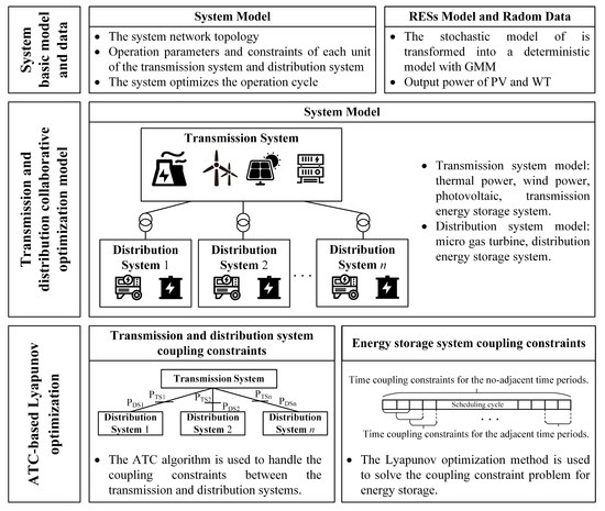
Figure 1. The proposed framework.

2.2. Modeling of Distribution System Optimization

For distribution systems, the distributed energy storage systems (DESSs), Micro gas Turbines (MTs) and system loads are considered. The DESSs in this paper are modeled based on small, distributed energy storage systems represented by lithium battery energy storages.

2.2.1. Objective Function

The objective function for the distribution system optimizes the output of the controllable units in the distribution system. For ESSs, this paper considers a combined operating cost, which includes the running cost and the levelized cost of the capital investments. The running cost is the cost of running the ESS in terms of per kilowatt-hour charging or discharging. By converting the costs of the ESS to per charging and discharging actions and daily operations, it is more suitable for the optimization of energy storage scheduling in this work.

The optimization objective is to minimize the total daily cost $C_{D,i}$ of the distribution system i, and the objective function can be formulated as

$$\min C_{D,i}=\frac{1}{T_0}(C_{D,i}^E+C_{D,i}^G+C_{D,i}^B),$$

(1)

$$C_{D,i}^E={\displaystyle \sum _{t=1}^{T_0}{\displaystyle \sum _{j=1}^{J_{DE}}{C}_{D,i,j,t}^E}}={\displaystyle \sum _{t=1}^{T_0}[c_{D,i,j}^{SE}+{\displaystyle \sum _{j=1}^{J_{DE}}{c}_{D,i,j}^E(P_{D,i,j,t}^{\mathrm{dis}}+P_{D,i,j,t}^{\mathrm{ch}})}],}$$

(2)

$$C_{D,i}^G={\displaystyle \sum _{t=1}^{T_0}{\displaystyle \sum _{j=1}^{J_{DG}}{C}_{D,i,j,t}^G}}={\displaystyle \sum _{t=1}^{T_0}{\displaystyle \sum _{j=1}^{J_{DG}}[c_{D,i,j}^{G,2}{(P_{D,i,j,t}^{\mathrm{G}})}^2+c_{D,i,j}^{G,1}{P}_{D,i,j,t}^{\mathrm{G}}+c_{D,i,j}^{G,0}],}}$$

(3)

$$C_{B,i}^G={\displaystyle \sum _{t=1}^{T_0}{c}_{TD,t}^T{P}_{D,i,t},}$$

(4)

where $C_{D,i}^E$, $C_{D,i}^G$ and $C_{D,i}^T$ represent the operating cost of the DESS in the distribution system i, the operating cost of MTs and the transaction cost of electricity with the transmission system, respectively; $C_{D,i,j,t}^E$ and $C_{D,i,j,t}^G$ represent the cost of the DESS j and the cost of MTs j in the distribution system i at time t, respectively; $c_{D,i,j}^E$ and $c_{D,i,j}^{SE}$ represent the MWh cost of the DESS j in the distribution system i and the levelized capital cost, respectively; $P_{D,i,j,t}^{\mathrm{dis}}$ and $P_{D,i,j,t}^{\mathrm{ch}}$ represent the discharging power and charging power of the DESS j in the distribution system i, respectively; $c_{D,i,j}^{G,2}$, $c_{D,i,j}^{G,1}$ and $c_{D,i,j}^{G,0}$ are the quadratic cost coefficient, primary cost coefficient and constant term cost coefficient of MTs j in the distribution system i; $P_{D,i,j,t}^{\mathrm{G}}$ represents the power generated by MTs j in the distribution system i; $c_{TD,t}^T$ represents the transaction price of the power transmission and distribution system at time t; $P_{D,i,t}$ represents the transaction power between the distribution system i and the transmission system at time t; $J_{DE}$ and $J_{DG}$ denote the number of DESSs and MTs in the distribution system i, respectively; $T_0$ is the solution period.

2.2.2. Constraints of Distribution System Optimization

The constraints of distribution system optimization mainly include power operation constraints, DESS constraints and MT operation constraints.

• Power Operation Constraints

The power operation constraints of the distribution system include the active power balance constraints of the distribution systems and the power exchange balance constraints between the transmission and distribution systems.

$$P_{D,i,t}+{\displaystyle \sum _j^{J_{DG}}{P}_{D,i,j,t}^{\mathrm{G}}}+{\displaystyle \sum _j^{J_{DE}}(P_{D,i,j,t}^{\mathrm{dis}}-P_{D,i,j,t}^{\mathrm{ch}})}={\displaystyle \sum _j^{J_{DL}}{P}_{D,i,j,t}^{\mathrm{L}},}$$

(5)

$$P_{T,i,t}+P_{D,i,t}=0,$$

(6)

where $P_{D,i,j,t}^{\mathrm{L}}$ represents the power of load j in the distribution system i at time t; $P_{T,i,t}$ represents the transaction power between the transmission system and distribution system i at time t.

2.

Operating Constraints of DESS

The constraints of DESSs mainly include upper- and lower-power-limit constraints and time-domain coupling constraints.

Among them, the time-domain coupling constraints include the State of Charge (SOC) constraints, SOC-limit constraints and the first and last SOC-equality constraints in the scheduling cycle.

$$0\le P_{D,i,j,t}^{\mathrm{dis}}\le M_{D,i,j,t}^{\mathrm{E}}{\overline{P}}_{D,i,j}^{\mathrm{E}},$$

(7)

$$0\le P_{D,i,j,t}^{\mathrm{ch}}\le (1-M_{D,i,j,t}^{\mathrm{E}}){\overline{P}}_{D,i,j}^{\mathrm{E}},$$

(8)

$$E_{D,i,j,t+1}=E_{D,i,j,t}+({\eta }_{D,i,j}^{\mathrm{E}}{P}_{D,i,j,t}^{\mathrm{ch}}-\frac{1}{{\eta }_{D,i,j}^{\mathrm{E}}}{P}_{D,i,j,t}^{\mathrm{dis}})\Delta t,$$

(9)

$${\underset{¯}{E}}_{D,i,j}\le E_{D,i,j,t}\le {\overline{E}}_{D,i,j},$$

(10)

$$E_{D,i,j,T}=E_{D,i,j,0},$$

(11)

where $M_{D,i,j,t}^{\mathrm{E}}$ is an indicator of the state of the DESS j in the distribution system i at time t, ‘1’ represents the discharge, and ‘0’ represents the charge; ${\overline{P}}_{D,i,j}^{\mathrm{E}}$ represents the maximum charging and discharging power of the DESS j in the power distribution system i; $E_{D,i,j,t}$ represents the SOC of the DESS j in the distribution system i at time t; ${\eta }_{D,i,j}^{\mathrm{E}}$ is the charging and discharging efficiency of the DESS j in the power distribution system i; ${\underset{\_}{E}}_{D,i,j}$ and ${\overline{E}}_{D,i,j}$ represent the minimum and maximum SOC of the DESS j in the distribution system i, respectively.

3.

Operating Constraints of MT

$$\{\begin{array}{ll}{\underset{\_}{P}}_{D,i,j}^{\mathrm{G}}\le P_{D,i,j,t}^{\mathrm{G}}\le {\overline{P}}_{D,i,j}^{\mathrm{G}},& (a)\\ {\underset{\_}{P}}_{D,i,j}^{\mathrm{GF}}\le |P_{D,i,j,t+1}^{\mathrm{G}}-P_{D,i,j,t}^{\mathrm{G}}|\le {\overline{P}}_{D,i,j}^{\mathrm{GF}},& (b)\end{array},$$

(12)

where ${\overline{P}}_{D,i,j}^{\mathrm{G}}$ and ${\underset{\_}{P}}_{D,i,j}^{\mathrm{G}}$ are the minimum and maximum power of the MT j in the distribution system i, respectively; ${\overline{P}}_{D,i,j}^{\mathrm{GF}}$ and ${\underset{\_}{P}}_{D,i,j}^{\mathrm{GF}}$ are the maximum and minimum ramp limits of the MT j in the distribution system i, respectively.

2.3. Modeling of the Transmission System Optimization

For the transmission system, the centralized energy storage systems (CESSs), renewable energy, thermal power (TP) units and grid loads are considered. The CESS this work considers is a large, centralized energy storage system represented by compressed air energy storage.

2.3.1. Objective Function

From the transmission system side, the optimization objective is to minimize the intraday operating cost $C_T$ of the transmission system, and the corresponding objective function is

$$\min C_T=\frac{1}{T_0}(C_T^E+C_T^G+C_T^R+C_T^T),$$

(13)

$$C_T^E={\displaystyle \sum _{t=1}^{T_0}{\displaystyle \sum _{j=1}^{J_{TE}}{C}_{T,j,t}^E}}={\displaystyle \sum _{t=1}^{T_0}[c_{T,j}^{SE}+{\displaystyle \sum _{j=1}^{J_{TE}}{c}_{T,j}^E(P_{T,j,t}^{\mathrm{dis}}+P_{T,j,t}^{\mathrm{ch}})}],}$$

(14)

$$C_T^R={\displaystyle \sum _{t=1}^{T_0}{\displaystyle \sum _{j=1}^{J_{RE}}{C}_{T,j,t}^R}}={\displaystyle \sum _{t=1}^{T_0}{\displaystyle \sum _{j=1}^{J_{RE}}[c_{T,j}^{PR}(P_{T,j,t}^{\mathrm{FR}}-P_{T,j,t}^{\mathrm{RE}})+c_{T,j}^R(P_{T,j,t}^{\mathrm{RE}})],}}$$

(15)

$$C_{T,i}^G={\displaystyle \sum _{t=1}^{T_0}{\displaystyle \sum _{j=1}^{J_{TG}}{C}_{T,j,t}^G}}={\displaystyle \sum _{t=1}^{T_0}{\displaystyle \sum _{j=1}^{J_{TG}}[c_{T,j}^{G,2}{(P_{T,i,t}^{\mathrm{G}})}^2+c_{T,j}^{G,1}{P}_{T,i,t}^{\mathrm{G}}+c_{T,j}^{G,0}],}}$$

(16)

$$C_T^T={\displaystyle \sum _{t=1}^{T_0}{c}_{TD,t}^T{P}_{T,i,t},}$$

(17)

where $C_T^E$, $C_T^G$, $C_T^R$ and $C_T^T$ are the total operating cost of the CESS in the transmission system, the total operating cost of renewable energy generations, the total operating cost of TP units and the transaction cost of electricity with the transmission system, respectively; $C_{T,j,t}^E$, $C_{T,j,t}^R$ and $C_{T,j,t}^G$ represent the operating costs of the CESS j, the operating cost of renewable energy j and the operating cost of the TP unit j at time t, respectively; $c_{T,j}^E$ and $c_{T,j}^{SE}$ indicate the MWh cost of the CESS j in the transmission system and the levelized capital cost, respectively; $P_{T,j,t}^{\mathrm{dis}}$ and $P_{T,j,t}^{\mathrm{ch}}$ represent the discharging power and charging power of the CESS j at time t; $c_{T,j}^{PR}$ and $c_{T,j}^R$ represent the penalty cost of the curtailment of renewable energy j and the converted unit operating cost of renewable energy j, respectively; $P_{T,j,t}^{\mathrm{FR}}$ and $P_{T,j,t}^{\mathrm{RE}}$ represent the maximum power and actual power of renewable energy j at time t; $c_{T,j}^{G,2}$, $c_{T,j}^{G,1}$ and $c_{T,j}^{G,0}$ represent the quadratic cost coefficient, primary cost coefficient and constant term cost coefficient of the TP unit j, respectively; $P_{T,i,t}^{\mathrm{G}}$ represents the generating power of the TP unit j at time t; $c_{TD,t}^T$ represents the transaction price between the transmission and distribution system at time t; $P_{D,i,t}$ represents the transaction power between the distribution system i and the transmission system at time t; $J_{TE}$, $J_{RE}$ and $J_{TG}$ are the number of CESSs, renewable energy and TP units, respectively.

2.3.2. Constraints of Transmission System Optimization

Similar to the constraints on distribution system optimization, transmission system optimization has the following operational constraints. Note that the uncertainty of renewable energy generation is handled by a Gaussian Mixture Model (GMM).

• Power Operation Constraints

These constraints include the power balance constraint of the transmission system and the interactive power balance constraints between the transmission and distribution systems.

$${\displaystyle \sum _j^{J_{TG}}{P}_{T,j,t}^{\mathrm{G}}}+{\displaystyle \sum _j^{J_{RE}}{P}_{T,j,t}^{\mathrm{RE}}}+{\displaystyle \sum _j^{J_{DE}}(P_{T,j,t}^{\mathrm{dis}}-P_{T,j,t}^{\mathrm{ch}})}={\displaystyle \sum _i^{I_{TD}}{P}_{T,i,t}}+{\displaystyle \sum _j^{J_{TL}}{P}_{T,j,t}^{\mathrm{L}},}$$

(18)

$${\displaystyle \sum _j^{J_{RE}}{P}_{T,j,t}^{\mathrm{RE}}}={\displaystyle \sum _j^{J_{TWT}}{P}_{T,j,t}^{\mathrm{WT}}}+{\displaystyle \sum _j^{J_{TPV}}{P}_{T,j,t}^{\mathrm{PV}},}$$

(19)

$$P_{T,i,t}+P_{D,i,t}=0,$$

(20)

where $P_{T,j,t}^{\mathrm{L}}$, $P_{T,j,t}^{\mathrm{WT}}$ and $P_{T,j,t}^{\mathrm{PV}}$ represent the actual power of load j, Wind Turbine (WT) j and Photovoltaic generator (PV) j, respectively, in the transmission system at time t; $J_{TL}$, $J_{TWT}$ and $J_{TPV}$ are the indices of the load, WT and PV in the transmission system.

2.

Operating Constraints of TP units

The TP units need to follow the power-limit constraints and ramp-limit constraints.

$$\left\{\begin{array}{l}{\underset{\_}{P}}_{T,j}^{\mathrm{G}}\le P_{T,j,t}^{\mathrm{G}}\le {\overline{P}}_{T,j}^{\mathrm{G}}\\ {\underset{\_}{P}}_{T,j}^{\mathrm{GF}}\le |P_{T,j,t+1}^{\mathrm{G}}-P_{T,j,t}^{\mathrm{G}}|\le {\overline{P}}_{T,j}^{\mathrm{GF}}\end{array}\right.,$$

(21)

where ${\overline{P}}_{T,j}^{\mathrm{G}}$ and ${\underset{\_}{P}}_{T,j}^{\mathrm{G}}$ denote the minimum and maximum power of the TP j; ${\overline{P}}_{T,j}^{\mathrm{GF}}$ and ${\underset{\_}{P}}_{T,j}^{\mathrm{GF}}$ are the maximum and minimum ramp limits of the TP j.

3.

Operating Constraints of CESS

The constraints of the CESS include upper- and lower-power-limit constraints and time-domain coupling constraints.

Among them, the time-domain coupling constraints include the SOC constraints, SOC upper-limit constraints and the first and last SOC equality constraints in the scheduling cycle.

$$0\le P_{T,j,t}^{\mathrm{dis}}\le M_{T,j,t}^{\mathrm{E}}{\overline{P}}_{T,j}^{\mathrm{E}},$$

(22)

$$0\le P_{T,j,t}^{\mathrm{ch}}\le (1-M_{T,j,t}^{\mathrm{E}}){\overline{P}}_{T,j}^{\mathrm{E}},$$

(23)

$$E_{T,j,t+1}^{}=E_{T,j,t}^{}+({\eta }_{T,j}^{\mathrm{E}}{P}_{T,j,t}^{\mathrm{ch}}-\frac{1}{{\eta }_{T,j}^{\mathrm{E}}}{P}_{T,j,t}^{\mathrm{dis}})\Delta t,$$

(24)

$${\underset{\_}{E}}_{T,j,t}^{}\le E_{T,j,t}^{}\le {\overline{E}}_{T,j}^{},$$

(25)

$$E_{T,j,T_0}^{}=E_{T,j,0}^{},$$

(26)

where the variables and constants are similar to the previously defined ones in Equations (7)–(11), and only the subscript “D” is replaced with “T” to represent the transmission.

4.

Renewable Energy Output Constraints

In this work, the GMM is used to describe the probability distribution of renewable energy output, and the Expectation Maximization (EM) algorithm is implemented to iteratively estimate the parameters in the GMM [19]. The EM algorithm can be divided into an E-step and an M-step, where the E-step estimates parameters based on current data and existing models and then uses the estimated parameter values to calculate the expected value of the likelihood function; the M-Step searches for the corresponding parameter when the likelihood function has the largest value. The E- and M-steps are repeated iteratively until the results of the parameters converge. Thereafter, the probability distribution of the maximum output power of renewable energy can be obtained.

The constraint in (27), which contains the random variable of the maximum predicted output of renewable energy, can be formulated as a chance constraint (28).

$$0\le P_{T,j,t}^{\mathrm{RE}}\le P_{T,j,t}^{\mathrm{FR}},$$

(27)

$$\mathrm{Pr}\{P_{T,j,t}^{\mathrm{RE}}\le P_{T,j,t}^{\mathrm{FR}}\}\ge 1-{\alpha }_{\mathrm{RE}},\mathrm{RE}\in (\mathrm{PV},\mathrm{WT}),$$

(28)

where $P_{T,j,t}^{\mathrm{RE}}$ represents the actual output power of the renewable energy j at time t; $P_{T,j,t}^{\mathrm{FR}}$ represents the maximum output power of the renewable energy j at time t; Pr{∗} represents the probability of event {∗}; $\tilde{\ast }$ represents the random variable of ∗; ${\alpha }_{\mathrm{RE}}$ represents the confidence of the corresponding chance constraint.

Further, the above chance constraints are transformed into deterministic constraints as follows:

$$0\le P_{T,j,t}^{\mathrm{RE}}\le Quant({\alpha }_{\mathrm{RE}}|P_{T,j,t}^{\mathrm{FR}})={\mathrm{CDF}}_P^{-1}({\alpha }_{\mathrm{RE}}),\mathrm{RE}\in (\mathrm{PV},\mathrm{WT}),$$

(29)

where $Quant({\alpha }_{\mathrm{RE}}|P_{T,j,t}^{\mathrm{FR}})$ is the quantile; ${\mathrm{CDF}}_P^{-1}({\alpha }_{\mathrm{RE}})$ represents the inverse function of the Cumulative Distribution Function (CDF).

Finally, Equation (29) can be solved by approximately fitting the CDF with a piecewise polynomial [19].

5.

The Uncertainty in the Cost of Energy

Besides the uncertainty of RES, the uncertainty in energy prices is also very important. With the increasing volatility of the international energy price, the uncertainties in the cost of energy have become the key to considering the economic optimization problem. To address this, [20,21] completed the relevant research excellently with comprehensive studies and analysis. Due to the limitation of space and the main scope of this work, this paper focuses on the co-optimizations of the ESSs in the transmission and distribution systems. Therefore, the optimization model in this work utilized the determined energy prices as inputs, which can be provided by the energy price forecasting results or can based on the uncertainty analysis results.

3. Model Transformation for Transmission–Distribution Co-Optimization

The distribution system optimization problem D1 for DESSs can be expressed as follows:

Objective function: (1);

Constraints: (5)–(12).

The optimization problem D1 is a mixed-integer linear programming problem. Constraint (1) is for the linearized objective function. Constraints (5), (6), (9) and (11) are equality constraints. Constraints (7), (8) and (12–b) are inequality constraints. Constraints (10) and (12–a) are the boundary constraints. All others are decision variables in real numbers except $M_{D,i,j,t}^{\mathrm{E}}$, which is a binary decision variable (0–1). The number of types of decision variables is seven, and the number of dimensions of decision variables depends on the number of resources in the system.

The transmission system optimization problem T1 for CESSs can be expressed as follows:

Objective function: (13);

Constraints: (18)–(26) and (29).

The optimization problem T1 is a mixed-integer linear programming problem. Constraint (13) is for the linearized objective function. Constraints (18), (19), (20), (24) and (26) are the equality constraints. Constraints (21–b), (22) and (23) are inequality constraints. Constraints (21–a), (25) and (29) are the boundary constraints. All others are decision variables in real numbers except $M_{T,j,t}^{\mathrm{E}}$, which is a binary decision variable (0–1). The number of types of decision variables is nine, and the number of dimensions of decision variables depends on the number of resources in the system.

Taking the distribution system optimization problem D1 as an example, the conversion method based on Lyapunov optimization is given below. The optimization problem of the transmission system T1 can be transformed in the same way as D1. Finally, the ATC-L is developed based on ATC, which solves the problem of collaborative optimization of the transmission system and distribution system considering the ESSs at both ends.

3.1. Model Transformation Based on Lyapunov Optimization

3.1.1. The Virtual Queue Stability Problem

Firstly, the energy storage virtual queue $Q_{D,i,j,t}$ is constructed with the time-domain coupling constraint (9) of the DESS:

$$Q_{D,i,j,t}=E_{D,i,j,t}^{}-{\beta }_D,$$

(30)

$$Q_{D,i,j,t+1}=Q_{D,i,j,t}+({\eta }_{D,i,j}^{\mathrm{E}}{P}_{D,i,j,t}^{\mathrm{ch}}-\frac{1}{{\eta }_{D,i,j}^{\mathrm{E}}}{P}_{D,i,j,t}^{\mathrm{dis}})\Delta t,$$

(31)

where ${\beta }_D$ is a constant. If ${\beta }_D$ satisfies the value range shown in (32), then the upper- and lower-limit-constraints of the DESS expressed in (10) are established.

Conclusion 1.

$${\underset{\_}{E}}_{D,i,j}^{}\le {\beta }_D\le {\overline{E}}_{D,i,j}^{}-{\eta }_{D,i,j}^{\mathrm{E}}{\overline{P}}_{D,i,j}^{\mathrm{E}}\Delta t-\frac{1}{{\eta }_{D,i,j}^{\mathrm{E}}}{\overline{P}}_{D,i,j}^{\mathrm{E}}\Delta t.$$

(32)

Proof of Conclusion 1.

 

Note that $E_{D,i,j,0}\in [{\underset{\_}{E}}_{D,i,j},{\overline{E}}_{D,i,j}]$ is known. It can be seen from Equation (30) that $Q_{D,i,j,0}\in [{\underset{\_}{E}}_{D,i,j}-{\beta }_D,{\overline{E}}_{D,i,j}-{\beta }_D]$ exists. In order to meet the constraint conditions represented by Equation (10), it is necessary to make further assumptions on the problem. First, assume that there is $E_{D,i,j,t}\in [{\underset{\_}{E}}_{D,i,j},{\overline{E}}_{D,i,j}]$, that is $Q_{D,i,j,t}\in [{\underset{\_}{E}}_{D,i,j}-{\beta }_D,{\overline{E}}_{D,i,j}-{\beta }_D]$; then we only need to prove $E_{D,i,j,t+1}\in [{\underset{\_}{E}}_{D,i,j},{\overline{E}}_{D,i,j}]$, that is $Q_{D,i,j,t+1}\in$ $[{\underset{\_}{E}}_{D,i,j}-{\beta }_D,{\overline{E}}_{D,i,j}-{\beta }_D]$; finally, the above conclusions have been proved.

The following will introduce the specific proof process:

First, prove that when $Q_{D,i,j,t}\le {\overline{E}}_{D,i,j}-{\beta }_D$ exists, $Q_{D,i,j,t+1}\le {\overline{E}}_{D,i,j}-{\beta }_D$ exists. According to the size of $Q_{D,i,j,t}$, there are two cases to prove:

• When $Q_{D,i,j,t}\in [{\underset{\_}{E}}_{D,i,j}-{\beta }_D,{\underset{\_}{E}}_{D,i,j}-{\beta }_D+{\overline{P}}_{D,i,j,t}\Delta t/{\eta }_{D,i,j}^{\mathrm{E}}]$, the DESS is in the charging state, and there are

$$\begin{array}{ll}{Q}_{D,i,j,t+1}& =Q_{D,i,j,t}+({\eta }_{D,i,j}^{\mathrm{E}}{P}_{D,i,j,t}^{\mathrm{ch}}-\frac{1}{{\eta }_{D,i,j}^{\mathrm{E}}}{P}_{D,i,j,t}^{\mathrm{dis}})\Delta t\\ & \le Q_{D,i,j,t}+{\eta }_{D,i,j}^{\mathrm{E}}{\overline{P}}_{D,i,j,t}\Delta t\\ & \le {\underset{\_}{E}}_{D,i,j}-{\beta }_D+\frac{1}{{\eta }_{D,i,j}^{\mathrm{E}}}{\overline{P}}_{D,i,j,t}\Delta t+{\eta }_{D,i,j}^{\mathrm{E}}{\overline{P}}_{D,i,j,t}\Delta t\\ & \le \frac{1}{{\eta }_{D,i,j}^{\mathrm{E}}}{\overline{P}}_{D,i,j,t}\Delta t+{\eta }_{D,i,j}^{\mathrm{E}}{\overline{P}}_{D,i,j,t}\Delta t\\ & ={\overline{E}}_{D,i,j}-{\overline{E}}_{D,i,j}+\frac{1}{{\eta }_{D,i,j}^{\mathrm{E}}}{\overline{P}}_{D,i,j,t}\Delta t+{\eta }_{D,i,j}^{\mathrm{E}}{\overline{P}}_{D,i,j,t}\Delta t\\ & \le {\overline{E}}_{D,i,j}-{\beta }_D\end{array}.$$

(33)

2.

When $Q_{D,i,j,t}\in ({\underset{\_}{E}}_{D,i,j}-{\beta }_D+{\overline{P}}_{D,i,j,t}\Delta t/{\eta }_{D,i,j}^{\mathrm{E}},{\overline{E}}_{D,i,j}-{\beta }_D].$, the DESS is in the discharge state, and there are

$$\begin{array}{ll}{Q}_{D,i,j,t+1}& =Q_{D,i,j,t}+({\eta }_{D,i,j}^{\mathrm{E}}{P}_{D,i,j,t}^{\mathrm{ch}}-\frac{1}{{\eta }_{D,i,j}^{\mathrm{E}}}{P}_{D,i,j,t}^{\mathrm{dis}})\Delta t\\ & =Q_{D,i,j,t}-\frac{1}{{\eta }_{D,i,j}^{\mathrm{E}}}{P}_{D,i,j,t}^{\mathrm{dis}}\Delta t\\ & \le Q_{D,i,j,t}\\ & \le {\overline{E}}_{D,i,j}-{\beta }_D\end{array}.$$

(34)

Second, prove that when $Q_{D,i,j,t}\ge {\underset{\_}{E}}_{D,i,j}-{\beta }_D$ exists, $Q_{D,i,j,t+1}\ge {\underset{\_}{E}}_{D,i,j}-{\beta }_D$ exists. Similarly, according to the size of $Q_{D,i,j,t}$, there are two cases to prove:

• When $Q_{D,i,j,t}\in [{\underset{\_}{E}}_{D,i,j}-{\beta }_D,{\underset{\_}{E}}_{D,i,j}-{\beta }_D+{\overline{P}}_{D,i,j,t}\Delta t/{\eta }_{D,i,j}^{\mathrm{E}}]$, the DESS is in the charging state, and there are

$$\begin{array}{ll}{Q}_{D,i,j,t+1}& =Q_{D,i,j,t}+({\eta }_{D,i,j}^{\mathrm{E}}{P}_{D,i,j,t}^{\mathrm{ch}}-\frac{1}{{\eta }_{D,i,j}^{\mathrm{E}}}{P}_{D,i,j,t}^{\mathrm{dis}})\Delta t\\ & =Q_{D,i,j,t}+{\eta }_{D,i,j}^{\mathrm{E}}{P}_{D,i,j,t}^{\mathrm{ch}}\Delta t\\ & \ge Q_{D,i,j,t}\\ & \ge {\underset{\_}{E}}_{D,i,j}-{\beta }_D\end{array},$$

(35)

2.

When $Q_{D,i,j,t}\in ({\underset{\_}{E}}_{D,i,j}-{\beta }_D+{\overline{P}}_{D,i,j,t}\Delta t/{\eta }_{D,i,j}^{\mathrm{E}},{\overline{E}}_{D,i,j}-{\beta }_D]$, the DESS is in the discharge state, and there are

$$\begin{array}{ll}{Q}_{D,i,j,t+1}& =Q_{D,i,j,t}+({\eta }_{D,i,j}^{\mathrm{E}}{P}_{D,i,j,t}^{\mathrm{ch}}-\frac{1}{{\eta }_{D,i,j}^{\mathrm{E}}}{P}_{D,i,j,t}^{\mathrm{dis}})\Delta t\\ & =Q_{D,i,j,t}-\frac{1}{{\eta }_{D,i,j}^{\mathrm{E}}}{P}_{D,i,j,t}^{\mathrm{dis}}\Delta t\\ & \ge {\underset{\_}{E}}_{D,i,j}-{\beta }_D+\frac{1}{{\eta }_{D,i,j}^{\mathrm{E}}}{\overline{P}}_{D,i,j,t}\Delta t-\frac{1}{{\eta }_{D,i,j}^{\mathrm{E}}}{P}_{D,i,j,t}^{\mathrm{dis}}\Delta t\\ & \ge {\overline{E}}_{D,i,j}-{\beta }_D\end{array}.$$

(36)

Therefore, Conclusion 1 has been proved.

Similarly, for the transmission system, there are the following equations:

$$Q_{T,j,t}=E_{T,j,t}-{\beta }_T,$$

(37)

$$Q_{T,j,t+1}=Q_{T,j,t}+({\eta }_{T,j}^{\mathrm{E}}{P}_{T,j,t}^{\mathrm{ch}}-\frac{1}{{\eta }_{T,j}^{\mathrm{E}}}{P}_{T,j,t}^{\mathrm{dis}})\Delta t,$$

(38)

$${\underset{\_}{E}}_{T,j}\le {\beta }_T\le {\overline{E}}_{T,j}-{\eta }_{T,j}^{\mathrm{E}}{\overline{P}}_{T,j}^{\mathrm{E}}\Delta t-\frac{1}{{\eta }_{T,j}^{\mathrm{E}}}{\overline{P}}_{T,j}^{\mathrm{E}}\Delta t,$$

(39)

where $Q_{T,j,t}$ represents the virtual queue of the CESS; ${\beta }_T$ is a constant, and its value range is given by Equation (39).

The time-domain coupling constraints of ESSs have been transformed into the stability problem of virtual queues. □

3.1.2. Transformation of Lyapunov Drift Penalty (L-DP) Function

In order to solve the above virtual queue stability problem, this subsection constructs the Lyapunov function which can characterize the virtual queue congestion degree. Furthermore, the model construction and solution of the virtual queue stability problem are realized.

First, the Lyapunov function can be constructed as

$${\mathit{Q}}_{D,i,t}={\displaystyle \sum _{j=1}^{J_{DE}}\frac{Q_{\mathrm{D},i,j,t}^2}{2}}.$$

(40)

When ${\mathit{Q}}_{D,i,t}$ is small, the virtual queues of all DESSs are less crowded, and the virtual queues are relatively more stable, and vice versa, i.e., when the virtual queues of DESSs are crowded, and the stability is poor.

Further, we define the Lyapunov Drift (L-D) function $\Delta {\mathit{Q}}_{D,i,t}$. The L-D function is used to characterize the difference of the degree of crowdedness between time t and time t + 1:

$$\Delta {\mathit{Q}}_{D,i,t}={\mathit{Q}}_{D,i,t+1}-{\mathit{Q}}_{D,i,t}.$$

(41)

It can be seen from the above equation that to stabilize the virtual queue represented by ${\mathit{Q}}_{D,i,t}$, the value of $\Delta {\mathit{Q}}_{D,i,t}$ needs be as small as possible. Thus, the original virtual queue stability problem is transformed into the minimization problem for $\Delta {\mathit{Q}}_{D,i,t}$.

Based on the L-DP function in [11], the problem of min.$\Delta {\mathit{Q}}_{D,i,t}$ transformed from the above virtual queue congestion problem is combined with the objective function of the optimization problem D1, which is

$$\min F_{D,i}=C_{D,i}+\Delta {\mathit{Q}}_{D,i,t},$$

(42)

where $\Delta {\mathit{Q}}_{D,i,t}$ has an upper bound, which can be expressed as

Conclusion 2.

$$\Delta {\mathit{Q}}_{D,i,t}\le {\displaystyle \sum _{j=1}^{J_{DE}}[Q_{D,i,j,t}({\eta }_{D,i,j}^{\mathrm{E}}{P}_{D,i,j,t}^{\mathrm{ch}}-\frac{1}{{\eta }_{D,i,j}^{\mathrm{E}}}{P}_{D,i,j,t}^{\mathrm{dis}})\Delta t]}.$$

(43)

Proof of Conclusion 2.

 

$$\begin{array}{ll}\Delta {\mathit{Q}}_{D,i,t}& ={\displaystyle \sum _{j=1}^{J_{DE}}(\frac{1}{2}{Q}_{D,i,j,t+1}^2-\frac{1}{2}{Q}_{D,i,j,t}^2)}\\ & =\frac{1}{2}{\displaystyle \sum _{j=1}^{J_{DE}}\{{[Q_{D,i,j,t}+({\eta }_{D,i,j}^{\mathrm{E}}{P}_{D,i,j,t}^{\mathrm{ch}}-\frac{1}{{\eta }_{D,i,j}^{\mathrm{E}}}{P}_{D,i,j,t}^{\mathrm{dis}})\Delta t]}^2-Q_{D,i,j,t}^2\}}\\ & ={\displaystyle \sum _{j=1}^{J_{DE}}[Q_{D,i,j,t}({\eta }_{D,i,j}^{\mathrm{E}}{P}_{D,i,j,t}^{\mathrm{ch}}-\frac{1}{{\eta }_{D,i,j}^{\mathrm{E}}}{P}_{D,i,j,t}^{\mathrm{dis}})\Delta t]}+{\displaystyle \sum _{j=1}^{J_{DE}}{[({\eta }_{D,i,j}^{\mathrm{E}}{P}_{D,i,j,t}^{\mathrm{ch}}-\frac{1}{{\eta }_{D,i,j}^{\mathrm{E}}}{P}_{D,i,j,t}^{\mathrm{dis}})\Delta t]}^2}\\ & \le {\displaystyle \sum _{j=1}^{J_{DE}}[Q_{D,i,j,t}({\eta }_{D,i,j}^{\mathrm{E}}{P}_{D,i,j,t}^{\mathrm{ch}}-\frac{1}{{\eta }_{D,i,j}^{\mathrm{E}}}{P}_{D,i,j,t}^{\mathrm{dis}})\Delta t]}+\frac{1}{2}{\displaystyle \sum _{j=1}^{J_{DE}}\{\max {[({\eta }_{D,i,j}^{\mathrm{E}}{P}_{D,i,j,t}^{\mathrm{ch}}-\frac{1}{{\eta }_{D,i,j}^{\mathrm{E}}}{P}_{D,i,j,t}^{\mathrm{dis}})\Delta t]}^2\}}\\ & \le {\displaystyle \sum _{j=1}^{J_{DE}}[Q_{D,i,j,t}({\eta }_{D,i,j}^{\mathrm{E}}{P}_{D,i,j,t}^{\mathrm{ch}}-\frac{1}{{\eta }_{D,i,j}^{\mathrm{E}}}{P}_{D,i,j,t}^{\mathrm{dis}})\Delta t]}\end{array}.$$

(44)

Based on the conclusion obtained from (43), the objective function (42) can be transformed into the following form:

$$\min F_{D,i}=C_{D,i}+{\displaystyle \sum _{j=1}^{J_{DE}}{Q}_{D,i,j,t}[({\eta }_{D,i,j}^{\mathrm{E}}{P}_{D,i,j,t}^{\mathrm{ch}}-\frac{1}{{\eta }_{D,i,j}^{\mathrm{E}}}{P}_{D,i,j,t}^{\mathrm{dis}})\Delta t]}.$$

(45)

Therefore, the original distribution system optimization problem D1 is transformed into the distribution system optimization problem D2:

Objective function: (45);

Constraints: (5)–(8) and (12).

Similarly, for the transmission system optimization problem T1, the same procedures can be used to transform T1 into the transmission system optimization problem T2. For the optimization problem T2, its objective function is

$$\min F_T=C_T+{\displaystyle \sum _{j=1}^{J_{TE}}{Q}_{T,j,t}[({\eta }_{T,j}^{\mathrm{E}}{P}_{T,j,t}^{\mathrm{ch}}-\frac{1}{{\eta }_{T,j}^{\mathrm{E}}}{P}_{T,j,t}^{\mathrm{dis}})\Delta t]},$$

(46)

where $Q_{T,j,t}$ is the virtual queue of CESSs in the transmission system.

Constraints: (18)–(23) and (29). □

3.2. Solution Model for the Transmission–Distribution System Co-Optimization Problem

There are consistency constraints in the optimization problem D2 and the optimization problem T2, namely, Equations (6) and (20). As a result, both optimization problems D2 and T2 have power constraints coupled with others, which cannot be solved independently.

The ATC method is mainly used to solve hierarchical, multi-agent coordinative optimization problems, which allows each optimization subject in the hierarchy to make independent decisions and, at the same time, coordinates the optimization to obtain the overall optimal solution of the problem. The basic idea of solving the transmission–distribution system co-optimization problem is in a hierarchical Bilevel Optimization, the transmission system optimization problem is considered a leader’s (upper-level) optimization problem, and the optimization problem of the distribution system is considered a follower’s (or lower-level) optimization problem. Both problems are solved independently first. Furthermore, the co-optimization is iteratively solved through the ATC method until the convergence condition is met. The ATC method has the advantages of parallelly solving the distributed optimization problem with sparse dependence and has rigorous proof of convergence [22].

Therefore, in this work, Equations (6) and (20) are relaxed to the objective functions of the optimization problems at each level in the form of penalty functions, so as to realize the complete decoupling and to provide independent optimization problems.

The distribution system optimization problem D2 is transformed into the optimization problem D3:

Objective function:

$$\min F_{D,i}=C_{D,i}+{\displaystyle \sum _{j=1}^{J_{DE}}{Q}_{D,j,t}[({\eta }_{D,i,j}^{\mathrm{E}}{P}_{D,i,j,t}^{\mathrm{ch}}-\frac{1}{{\eta }_{D,i,j}^{\mathrm{E}}}{P}_{D,i,j,t}^{\mathrm{dis}})\Delta t]}+{\displaystyle \sum _{t=1}^{T_0}[v_{i,t}({\widehat{P}}_{T,i,t}-P_{D,i,t})+w_{i,t}{({\widehat{P}}_{T,i,t}-P_{D,i,t})}^2]};$$

(47)

Constraints: (5), (7), (8) and (12).

The transmission system optimization problem T2 is transformed into the optimization problem T3:

$$\min F_T=C_T+{\displaystyle \sum _{j=1}^{J_{TE}}{Q}_{T,j,t}[({\eta }_{T,j}^{\mathrm{E}}{P}_{T,j,t}^{\mathrm{ch}}-\frac{1}{{\eta }_{T,j}^{\mathrm{E}}}{P}_{T,j,t}^{\mathrm{dis}})\Delta t]}+{\displaystyle \sum _{i=1}^{I_{TD}}{\displaystyle \sum _{t=1}^{T_0}[v_{i,t}(P_{T,i,t}-{\widehat{P}}_{D,i,t})+w_{i,t}{(P_{T,i,t}-{\widehat{P}}_{D,i,t})}^2]}};$$

(48)

Constraints: (18), (19), (21)–(23) and (29).

In the above equations, ${\widehat{P}}_{T,i,t}$ and ${\widehat{P}}_{D,i,t}$ represent the amount of exchange power, calculated by the optimization of the distribution system and the transmission system, respectively, which are known values; $v_{i,t}$ and $w_{i,t}$, respectively, represent the multiplier coefficients of the primary and quadratic terms of the penalty function, and the update rule is

$$\left\{\begin{array}{l}{v}_{i,t,k+1}=v_{i,t,k}+2{(w_{i,t,k})}^2(P_{T,i,t,k}-P_{D,i,t,k})\\ w_{i,t,k+1}=\lambda w_{i,t,k}\end{array}\right.,$$

(49)

where k is the number of iterations; λ is a coefficient constant, generally taking the value between 1 and 3.

The convergence condition is

$$\left\{\begin{array}{l}\left|P_{T,i,t,k}-P_{D,i,t,k}\right|\le {\epsilon }_1,\forall t\in T_0,\forall i\in I_{TD}\\ \left|\frac{C_{T,k}+{\displaystyle \sum _{i=1}^{I_{TD}}{C}_{D,i,k}}-(C_{T,k-1}+{\displaystyle \sum _{i=1}^{I_{TD}}{C}_{D,i,k-1}})}{C_{T,k}+{\displaystyle \sum _{i=1}^{I_{TD}}{C}_{D,i,k}}}\right|\le {\epsilon }_2\end{array}\right.,$$

(50)

where both ${\epsilon }_1$ and ${\epsilon }_1$ represent the convergence coefficients.

Based on the above formulations, the pseudo code of the proposed ATC-L in this paper is presented in Algorithm 1. The assumptions of the ATC-L algorithm are as follows:

First, in the optimization scenario, the algorithm proposed in this paper is applicable to the linear convex optimization problem for the ESSs. In addition, the optimization problem should be a day-ahead scheduling problem or have a fixed scheduling cycle. In the problem of transmission and distribution co-optimization, this paper is only set to optimize the scheduling of the real power.

Second, in the optimization model, the ESSs that should be considered by the proposed algorithm in this paper needs to have SOC operating constraints and SOC upper- and lower-limit constraints, and the initial SOC should be equal to the last SOC for a fixed scheduling cycle.

The ATC-L algorithm proposed in this paper takes the ATC algorithm as the basic framework, integrates the energy storage coupling constraint decoupling problem based on the Lyapunov optimization and further improves the ATC algorithm. Through the relevant algorithm procedures in the pseudo code, it is not difficult to find that the convergence of the ATC-L algorithm and the convergence of the ATC algorithm are built on the same mathematical foundation, and the decoupling of the energy storage coupling constraint does not affect the convergence problem. Refs [22,23] have also pointed out that the ATC algorithm has good convergence in multi-level optimization problems. Therefore, the ATC-L algorithm can also converge when solving similar convex optimization problems.

Algorithm 1. The pseudo code of ATC-L.

Algorithm 1: Analytical target cascading based on Lyapunov optimization (ATC-L)

Input: Optimization problem D3 and T3 model. Output: Optimal Solution for the Collaborative Optimization of Transmission System and Distribution System. ${\widehat{P}}_{T,i,t,k}=P_{T,i,t,0},\forall t\in T_0,\forall i\in I_{TD}$; // Set the transmission system’s initial active injection power; k = 0; // Initialize the number of iterations; Initialize the convergence coefficients ε1 and ε2, and the multiplier coefficients $v_{i,t,0}$ and $w_{i,t,0}$; while (Equation (50) set up ) do;   for (t = 1 to T0 ) do;    According to the virtual queue QT(t), calculate the optimal solution of the transmission system optimization problem T3;    Update the virtual queue QT(t);   end for;    ${\widehat{P}}_{D,i,t,k}=P_{D,i,t,k},\forall t\in T_0,\forall i\in I_{TD}$; // Update the distribution system switching power ${\widehat{P}}_{D,i,t}$ according to the optimization result of Step7;   for (t = 1 to T0 ) do;    According to the virtual queue QD(t), the optimization problem D3 optimal solution of all distribution systems is calculated in parallel    Update the virtual queue QD(t) in parallel;   end for;    ${\widehat{P}}_{T,i,t,k}=P_{T,i,t,k},\forall t\in T_0,\forall i\in I_{TD}$; // Update the transmission system switching power ${\widehat{P}}_{T,i,t}$ according to the optimization result of Step12;   Update the multiplier coefficients $v_{i,t,k}$ and $w_{i,t,k}$ according to Equation (49);   k = k + 1; end while; return $\mathit{C}=[C_T,C_{D,i},\dots ,C_{D,I_{TD}}],\mathit{P}=[P_T,P_{D,i},\dots ,P_{D,I_{TD}}]$.

4. Case Studies

In this work, the 24-h day-ahead scheduling is taken as a test scenario to verify the feasibility and effectiveness of the proposed ATC-L algorithm and the co-optimization of the transmission–distribution systems with ESSs at both ends. The simulations are performed with MATLAB-2022A, Intel (R) Core (TM) i5-12400 CPU and the commercial solver Cplex-12.10.0.

4.1. The Test Scenario

The T6D7 system is selected, which includes a 6-node transmission network and three 7-node active distribution networks. The network topology and resource configuration of each active distribution network are the same, but the resource configuration parameters are different. Figure 2 shows the resource configuration and system structure in the system. Figure 3 shows the price of transmission and distribution transactions. Table 1 gives the parameters of the ESSs and other resources in the system. Table 2 gives the ESSs’ cost [24], wind and solar curtailment cost [25,26] and other resource cost parameters [27].

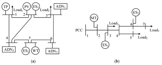
Figure 2. The single-line diagram of the T6D7 system: (a) the single-line diagram of the transmission system; (b) the single-line diagram of the distribution system.

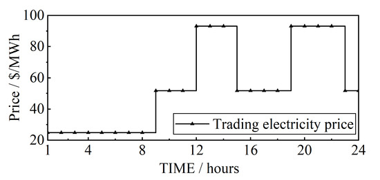
Figure 3. The transmission and distribution systems’ electricity trading price (USD).

Table 1. The system resources’ parameter configuration.

	Transmission System		Distribution System
ESS Number	T_1	T_2	D_1			D_2			D_3
Rated Power/MW	150	200	15	20		10	15		15	20
Rated Capacity/MWh	750	1200	30	40		30	45		15	40
Efficiency	65%	65%	85%	85%		85%	85%		85%	85%
Initial SOC	50%	50%	50%	50%		50%	50%		50%	50%
Minimum SOC	10%	10%	20%	20%		20%	20%		20%	20%
Maximum SOC	90%	90%	80%	80%		80%	80%		80%	80%
Unit Type	TP		MT_1			MT_2			MT_3
Rated Power/MW	300		20			25			15
Minimum Power/MW	100		0			0			0
Climbing Limit/MW/h	±100		±10			±10			±5
Unit Type	PV	WT	/
Rated Power/MW	450	450
Load Number	T_1	T_2	D_1	D_2	D_3	D_4	D_5	D_6	D_7	D_8	D_9
Load Ratio/MW	223	275	5	10	5	10	5	5	10	5	5

Table 2. The costs of each resource in the system.

	Transmission System		Distribution System
ESS Number	T_1	T_2	D_1	D_2	D_3
Cost Per MWh/USD/MWh	62.92		105.82
Fixed Cost/USD/MW/day	78.28		104.37
Unit Type	TP		MT_1	MT_2	MT_3
Quadratic Cost Coefficient/USD/MW2	0.41		1.08	1.11	1.43
Primary Cost Coefficient/USD/MW	11.26		29.31	27.13	25.94
Constant Term Cost/USD/day	2164		1120	1041	1100
Unit Type	PV	WT	/
Daily Operating Cost/MW	144.60
Unit Curtailment Penalty Cost/USD/MW	503.50	555.60

In order to validate of the ATC-L algorithm in complex scenarios, this paper also tested the proposed algorithm with a T30D22 system, which includes a 30-bus transmission network and four 22-bus distribution networks and a T118D141 system, which includes a 118-bus transmission network and five 141-bus distribution networks. The topology of each system is described in [10]. The system configurations are shown in Table 3. All resource parameters in the system are configured according to the T6D7 system. Because we set 15 ESSs in each distribution network of the T118D141 system, the energy storage systems numbered 1,4,7,10 and 13 are the same as the energy storage system D_1 in Table 1 and Table 2. This is the same for the parameters of other sources.

Table 3. The systems’ parameter configuration.

	Transmission System		Distribution System
Number of nodes	30	118	22	141
Number of ESSs	5	15	5	15
Number of TP	2	6	/
Number of PV	2	6	/
Number of WT	2	6	/
Number of MT	/		3	9
Number of Load	5	15	5	20

The relevant parameters for the ATC-L are set as follows. Both ${\beta }_D$ and ${\beta }_T$ select the maximum value within their range [12,13]. According to Equations (32) and (39), it can be seen that the values of ${\beta }_D$ and ${\beta }_T$ are 4.47 and 76.231. The algorithm convergence coefficients ${\epsilon }_1$ and ${\epsilon }_2$ are both set as 0.01. The initial values of the coefficients $v_{i,t}$ and $w_{i,t}$ of the primary and secondary term multipliers of the penalty function are both set as 0.01. Lastly, λ is 1.5.

In order to further verify the effectiveness of the proposed ATC-L algorithm, the following 10 groups of cases are simulated.

4.2. Analysis of Optimization Results

The algorithm convergence process of Case C1 is shown in Figure 4. It can be seen from the figure that the proposed algorithm converges after nine iterations, and the exchange power between the transmission system and the distribution system tends to be consistent. Specifically, as the number of iterations increases, the exchange power penalty increases, the power coupling constraints between the transmission system and the distribution systems are gradually tightened, and the system boundary interaction power gradually converges.

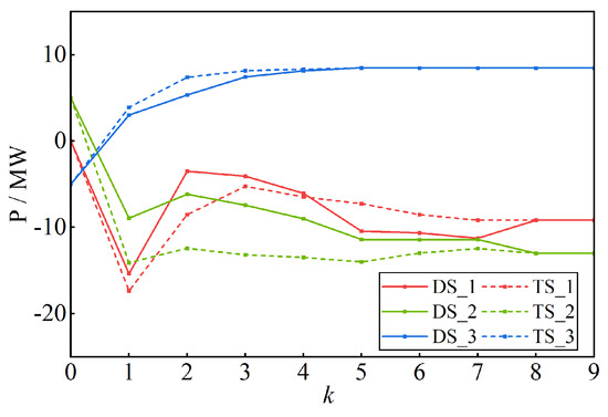
Figure 4. The boundary power convergence process.

The system operation results of Case C1 and the SOC changes of the ESSs are shown in Figure 5 and Figure 6. During the time period from 01:00 to 08:00, the output of renewable energy generations can basically meet the load demand in the grid. Furthermore, due to the penalty cost of the curtailment of renewable energy, the consumption rate of renewable energy is relatively high. During this time period, the TP units and MT units in the grid maintain the minimum output. Moreover, due to the low operating cost of the CESS in the transmission system, the CESS is more involved in discharging during this period to supply the grid loads that were not fully supplied by the renewable energy generations and the transaction power from the distribution system.

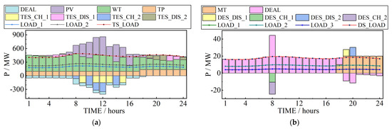
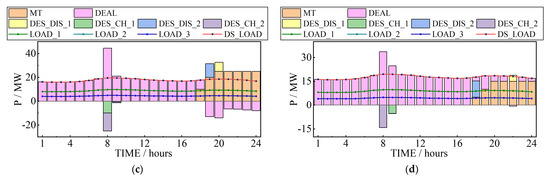
Figure 5. The simulation results of the system operations: (a) the transmission system; (b) distribution system 1; (c) distribution system 2; (d) distribution system 3.

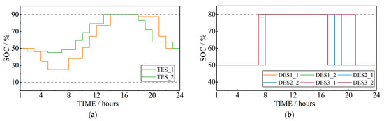
Figure 6. The SOC curves of the ESSs: (a) the transmission system; (b) the distribution systems.

When the system’s renewable energy power generation reaches its peak period (09:00–17:00), the output of renewable energy resources can fully meet the load demand in the grid. During this time period, the TP units and MT units in the grid also maintain the minimum output. Due to the high-power generation of renewable energy resources at this time, all ESSs on both sides of the transmission system and distribution system are in charging states. Furthermore, the SOCs of all ESSs increase. Renewable energy has been accommodated. During the second time period from 18:00 to 24:00, the output of the renewable energy generations cannot meet the load demand in the grid. During this period, the output of the TP units and MT units in the system increase. At the beginning of this period, the SOCs of the ESSs in the transmission system and the distribution systems are still at a relatively high level due to the charging from the renewable energy generations during the peak output period. During this period, the grid reaches its peak demand and the ESSs on both the transmission and distribution sides provide power to the grid through discharging to meet the system load demand. The SOCs of all ESSs at the end of the 24 h dispatching period are equal to the initial SOCs. This operation constraint improves the scheduling capability of the energy storage system in multiple operating cycles.

Note that the optimization cycles are not limited to 24 h; it can also be 48- or 72 h, which depends on the needs of the operators. The optimal length of the cycle in terms of accurate and efficient operation scheduling of ESSs could depend on the trade off with energy forecasting accuracies, considering uncertainties.

Figure 7 shows the consumption of renewable energy under different ESS configurations, and Table 4 shows the corresponding costs of each case. Through the above results, it can be seen that the grid-connected ESSs on both sides of the transmission and distribution have effectively improved the renewable energy hosting capacity of the system and reduced the operating costs of the system.

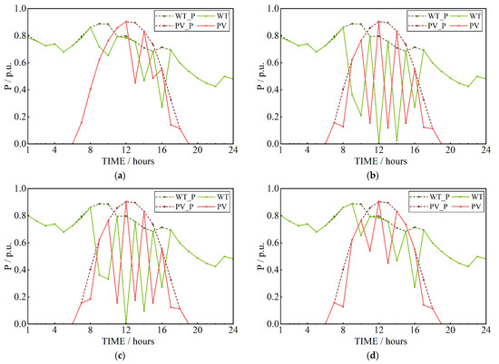
Figure 7. The usage comparison of renewable energy: (a) Case C1; (b) Case C2; (c) Case C3; (d) Case C4.

Table 4. Case configurations.

Case Number	Algorithm Settings	Energy Storage System Configuration
C-A1	ATC-L	Transmission and Distribution Systems
C-A2	ATC-L	Without ESSs
C-A3	ATC-L	Transmission System Only
C-A4	ATC-L	Distribution System Only
C-A5	ATC	Transmission and Distribution Systems
C-A6	Centralized Optimization	Transmission and Distribution Systems
C-B2	ATC-L	Transmission and Distribution Systems
C-B2	ATC	Transmission and Distribution Systems
C-C3	ATC-L	Transmission and Distribution Systems
C-C3	ATC	Transmission and Distribution Systems

From the optimization results of the different cases given in Table 5, it can be seen that the ATC-L proposed in this paper effectively reduces the system operating cost compared with the original ATC, and the error of the cost with respect to the centralized optimization method is 0.0694%.

Table 5. The costs of the transmission system and the distribution systems.

Case No.	MT Cost/USD	DESS Cost/USD	CESS Cost/USD	RECPC 1/USD	REFC 2/USD	TP Cost/USD	Total Cost/USD
C1	97,125.3	13,492.7	141,556.7	130,291.1	476,595.0	205,772.0	1,064,832.8
C2	102,898.0	0	0	370,138.6	476,595.0	298,748.4	1,248,380.0
C3	102,260.1	27,684.0	0	348,673.5	476,595.0	283,298.9	1,238,511.5
C4	97,125.3	0	141,556.7	140,498.1	476,595.0	212,243.8	1,068,019.9
C5	97,125.3	13,492.7	132,512.0	162,856.2	476,595.0	197,359.6	1,079,941.9
C6	97,125.3	13,492.7	142,042.7	128,631.3	476,595.0	206,207.8	1,064,094.8

¹ RECPC (Renewable Energy Curtailment Penalty Cost); ² REFC (Renewable Energy Fixed Cost).

4.3. Large-Scale System Analysis

Cases C-B and C-C in this paper are designed to verify the applicability of the ATC-L algorithm in large-scale systems.

Figure 8 and Figure 9 show the calculation results of Cases C-B1 and C-C1, respectively, and show the operation of ESSs and the corresponding SOCs in the system.

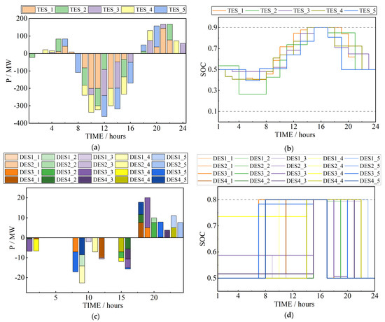
Figure 8. The simulation results of Case C-B1 system operations: (a) ESSs in the transmission system; (b) the SOC curves of ESSs in the transmission system; (c) ESSs in the distribution systems; (d) the SOC curves of ESSs in the distribution systems.

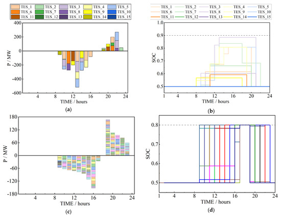
Figure 9. The simulation results of Case C-C1 system operations: (a) ESSs in the transmission system; (b) the SOC curves of ESSs in the transmission system; (c) ESSs in the distribution systems; (d) the SOC curves of ESSs in the distribution systems.

Table 6 presents the calculation time consummations for Cases C-A1, C-A5, C-B1, C-B2, C-C1 and C-C2. It is obvious that the calculation time increases as the scale of the system increases.

Table 6. Comparison of the computation time of the different cases.

Case No.	C-A1	C-A5	C-B1	C-B2	C-C1	C-C2
The computation time/s	2.79	4.29	4.83	9.10	16.00	46.10

From the comparison of the ATC algorithm and the ATC-L algorithm, it can be seen that the ATC-L algorithm can better deal with the system with more ESSs. Moreover, with the increase of the system scale, the performance advantages of the ATC-L algorithm are more obvious. The reason is that the ATC-L algorithm can deal with the ESS time-domain coupling constraints and can decouple them to simplify and accurately solve the optimization problem.

4.4. Sensitivity Analysis

4.4.1. The Energy Storage Price Sensitivity Analysis

As the price of ESSs is still high, the benefit brought by using ESSs to improve the consumption of renewable energy is not obvious. With the continuous development and maturity of energy storage technology in the future, the cost will be further reduced. This paper sets 10 energy storage cost multipliers and gives the sensitivity analysis of different energy storage cost multipliers to the system operating cost and renewable energy consumption. The operational cost of the system is reflected through the total cost, and the consumption of renewable energy is reflected through the CPC. Figure 10 presents the corresponding results. It can be intuitively found from the figure that as the price of the ESSs drops, the penalty cost reduction of the system and the total operating cost of the system both decrease. This also further shows that the configuration of ESSs can effectively promote the consumption of renewable energy, reduce the power generation of traditional thermal power units and improve the economics of the overall operations of the transmission and distribution systems.

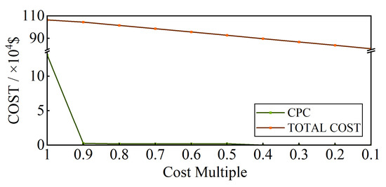
Figure 10. The system total cost and CPC under different energy storage cost multipliers (USD).

4.4.2. Effect of Different Confidence Levels on Cost

This section presents the impacts of different confidence levels of renewable energy output on the costs of operations. The basic parameters of Case C1 are used. It can be seen from the results in Table 7 that as the confidence level decreases, the operating cost of the system decreases.

Table 7. The system cost at different confidence levels.

Confidence	MT Cost/USD	DESS Cost/USD	TESS Cost/USD	CPC/USD	REFC/USD	TP Cost/USD	Total Cost/USD
0.99	97,125.3	13,492.7	118,398.4	282,522.00	476,595.0	187,273.3	1,175,406.7
0.95	97,125.3	13,492.7	125,131.9	218,184.5	476,595.0	195,117.1	1,125,646.4
0.9	97,125.3	13,492.7	141,556.7	130,291.1	476,595.0	205,772.0	1,064,832.8
0.85	97,173.2	13,492.7	167,500.0	335,73.6	476,595.0	217,266.3	1,005,600.9
0.8	104,418.8	626.2	162,588.4	0	476,595.0	234,465.4	978,693.8

5. Conclusions

In this work, a hierarchical optimization framework is proposed for the co-optimization of the power transmission system and multiple distribution systems considering the ESSs at both ends of the systems. An ATC-L algorithm is developed for solving the transmission–distribution system co-optimization problem with parallel computations and the decoupling of the operational constraints of the system. The Lyapunov optimization is integrated into the ATC-L algorithm to realize the decoupling of the time-domain coupling constraints of ESSs. The case studies showed that the proposed methods can effectively save the cost of operations of ESSs and improve the hosting capacity and utilization of the renewable energy resources. A sensitivity analysis was also performed in terms of the impact of the energy storage price on the operating cost of the system and the renewable energy. The results show that further development of energy storage technology and the corresponding investment reduction can greatly improve the transition from fossil fuel-based generations to renewable energies.

References

- Golombek, R.; Lind, A.; Ringkjøb, H.K.; Seljom, P. The role of transmission and energy storage in European decarbonization towards 2050. Energy 2022, 239, 122159. [Google Scholar] [CrossRef]
- Rahman, M.A.; Kim, J.H.; Hossain, S. Recent advances of energy storage technologies for grid: A comprehensive review. Energy Storage 2022, 4, e322. [Google Scholar] [CrossRef]
- Chen, S.; Li, Z.; Li, W. Integrating high share of renewable energy into power system using customer-sited energy storage. Renew. Sustain. Energy Rev. 2021, 143, 110893. [Google Scholar] [CrossRef]
- Arteaga, J.; Zareipour, H.; Amjady, N. Energy storage as a service: Optimal pricing for transmission congestion relief. IEEE Open Access J. Power Energy 2020, 7, 514–523. [Google Scholar] [CrossRef]
- Li, X.; Wang, S. Energy management and operational control methods for grid battery energy storage systems. CSEE J. Power Energy Syst. 2019, 7, 1026–1040. [Google Scholar] [CrossRef]
- Xue, G.; Wu, C.; Xu, Z.; Liu, Z. An Economic study of Power Secondary Frequency Regulation with Different Energy Storage Systems. In Proceedings of the 2022 IEEE 5th International Electrical and Energy Conference (CIEEC), Nanjing, China, 27–29 May 2022; IEEE: Piscataway, NJ, USA, 2022; pp. 4448–4454. [Google Scholar] [CrossRef]
- Liu, J.; Hu, H.; Yu, S.S.; Trinh, H. Virtual Power Plant with Renewable Energy Sources and Energy Storage Systems for Sustainable Power Grid-Formation, Control Techniques and Demand Response. Energies 2023, 16, 3705. [Google Scholar] [CrossRef]
- Mi, Y.; Chen, Y.; Yuan, M.; Li, Z.; Tao, B.; Han, Y. Multi-Timescale Optimal Dispatching Strategy for Coordinated Source-Grid-Load-Storage Interaction in Active Distribution Networks Based on Second-Order Cone Planning. Energies 2023, 16, 1356. [Google Scholar] [CrossRef]
- Leon, J.I.; Dominguez, E.; Wu, L.; Alcaide, A.M.; Reyes, M.; Liu, J. Hybrid energy storage systems: Concepts, advantages, and applications. IEEE Ind. Electron. Mag. 2020, 15, 74–88. [Google Scholar] [CrossRef]
- Zhang, T.; Wang, J.; Wang, H.; Ruiyang, J.; Li, G.; Zhou, M. On the coordination of transmission-distribution grids: A dynamic feasible region method. IEEE Trans. Power Syst. 2022, 38, 1855–1866. [Google Scholar] [CrossRef]
- Neely, M.J. Stochastic network optimization with application to communication and queueing systems. Synth. Lect. Commun. Netw. 2010, 3, 1–211. [Google Scholar]
- Li, P.; Sheng, W.; Duan, Q.; Li, Z.; Zhu, C.; Zhang, X. A Lyapunov optimization-based energy management strategy for energy hub with energy router. IEEE Trans. Smart Grid 2020, 11, 4860–4870. [Google Scholar] [CrossRef]
- Fan, S.; Liu, J.; Wu, Q.; Cui, M.; Zhou, H.; He, G. Optimal coordination of virtual power plant with photovoltaics and electric vehicles: A temporally coupled distributed online algorithm. Appl. Energy 2020, 277, 115583. [Google Scholar] [CrossRef]
- Rajaei, A.; Fattaheian-Dehkordi, S.; Fotuhi-Firuzabad, M.; Moeini-Aghtaie, M. Decentralized transactive energy management of multi-microgrid distribution systems based on ADMM. Int. J. Electr. Power Energy Syst. 2021, 132, 107126. [Google Scholar] [CrossRef]
- Chen, Z.; Li, Z.; Guo, C.; Wang, J.; Ding, Y. Fully distributed robust reserve scheduling for coupled transmission and distribution systems. IEEE Trans. Power Syst. 2020, 36, 169–182. [Google Scholar] [CrossRef]
- Dung, N.V.; Trung, N.L.; Abed-Meraim, K. Robust subspace tracking with missing data and outliers: Novel algorithm with convergence guarantee. IEEE Trans. Signal Process. 2021, 69, 2070–2085. [Google Scholar] [CrossRef]
- Nawaz, A.; Wang, H. Distributed stochastic security constrained unit commitment for coordinated operation of transmission and distribution system. CSEE J. Power Energy Syst. 2020, 7, 708–718. [Google Scholar] [CrossRef]
- Wang, Y.; Yu, Z.; Dou, Z.; Qiao, M.; Zhao, Y.; Xie, R.; Liu, L. Decentralized Coordination Dispatch Model Based on Chaotic Mutation Harris Hawks Optimization Algorithm. Energies 2022, 15, 3815. [Google Scholar] [CrossRef]
- Wang, Z.; Shen, C.; Liu, F.; Wu, X.; Liu, C.C.; Gao, F. Chance-constrained economic dispatch with non-Gaussian correlated wind power uncertainty. IEEE Trans. Power Syst. 2017, 32, 4880–4893. [Google Scholar] [CrossRef]
- Scarabaggio, P.; Grammatico, S.; Carli, R.; Dotoli, M. Distributed demand side management with stochastic wind power forecasting. IEEE Trans. Control Syst. Technol. 2021, 30, 97–112. [Google Scholar] [CrossRef]
- Scarabaggio, P.; Carli, R.; Dotoli, M. Noncooperative Equilibrium-Seeking in Distributed Energy Systems Under AC Power Flow Nonlinear Constraints. IEEE Trans. Control Netw. Syst. 2022, 9, 1731–1742. [Google Scholar] [CrossRef]
- Tosserams, S.; Etman, L.F.P.; Papalambros, P.Y.; Rooda, J.E. An augmented Lagrangian relaxation for analytical target cascading using the alternating direction method of multipliers. Struct. Multidiscip. Optim. 2006, 31, 176–189. [Google Scholar] [CrossRef]
- Michelena, N.; Park, H.; Papalambros, P.Y. Convergence properties of analytical target cascading. AIAA J. 2003, 41, 897–905. [Google Scholar] [CrossRef]
- Mongird, K.; Viswanathan, V.; Balducci, P.; Alam, J.; Fotedar, V.; Koritarov, V.; Hadjerioua, B. An Evaluation of Energy Storage Cost and Performance Characteristics. Energies 2020, 13, 3307. [Google Scholar] [CrossRef]
- Liu, G.; Tomsovic, K. Quantifying spinning reserve in systems with significant wind power penetration. IEEE Trans. Power Syst. 2012, 27, 2385–2393. [Google Scholar] [CrossRef]
- Morales, J.M.; Conejo, A.J.; Pérez-Ruiz, J. Economic valuation of reserves in power systems with high penetration of wind power. IEEE Trans. Power Syst. 2009, 24, 900–910. [Google Scholar] [CrossRef]
- Iacobucci, R.; McLellan, B.; Tezuka, T. The Synergies of Shared Autonomous Electric Vehicles with Renewable Energy in a Virtual Power Plant and Microgrid. Energies 2018, 11, 2016. [Google Scholar] [CrossRef]
Disclaimer/Publisher’s Note: The statements, opinions and data contained in all publications are solely those of the individual author(s) and contributor(s) and not of MDPI and/or the editor(s). MDPI and/or the editor(s) disclaim responsibility for any injury to people or property resulting from any ideas, methods, instructions or products referred to in the content. |
© 2023 by the authors. Licensee MDPI, Basel, Switzerland. This article is an open access article distributed under the terms and conditions of the Creative Commons Attribution (CC BY) license (https://creativecommons.org/licenses/by/4.0/).