Abstract
Floating Photovoltaic (FPV) plants are already well developed, and deployed all over the world, on calm water inland lakes, or in sheltered locations. They are now progressing to be installed in nearshore sites, and in deep water seas. The company HelioRec, developing floating modules to form FPV arrays to be deployed in nearshore areas, was awarded free-of-charge testing of their system by the Marine Energy Alliance (MEA) European program. This paper describes the experimental testing of the 1:1 scale float system, composed of 16 floating modules supporting solar panels and three footpaths, carried out in Centrale Nantes’ ocean wave tank, allowing regular and irregular frontal and oblique wave conditions. Experimental results show that, even in the narrow wave spectrum experimentally achievable, a specific response from the array was revealed: the multibody articulated system exhibits a first-order pitch resonant mode when wavelengths are about twice the floater length. A shadowing effect, leading to smaller motions of rear floaters, is also observed, for small wavelengths only.
1. Introduction
In 2021, the U.S. Energy Information Administration predicted, assuming current policy and technology trends to continue, a nearly 50% increase in energy demand in 2050 compared to 2020, primarily due to population and economic growth, particularly in Asia [1]. Renewable energies are expected to be producing around 27% of worldwide energy production in 2050, a 165% increase compared to 2020 levels.
Amongst renewable energies, solar energy captured by photovoltaic (PV) panels is now recognised as one of the most reliable sources of energy. The sector’s worldwide installed capacity grew from small-scale applications totalling 10.5 GW in 2008 to a mainstream energy production sector in 2021 with 940 GW installed [2], as the module prices decreased to 0.30 USD/Wp in 2018, a drop of nearly 99.6% since 1976 [3]. Yet, the sector’s expansion is limited by its large requirement of land space, making it compete with traditional uses of land, like agriculture.
In order to avoid this limitation, Floating Photovoltaic (FPV) plants have been developed in many parts of the world, primarily on relatively calm free-surface water areas such as inland lakes and hydropower reservoirs. Their main advantages are an increased power production due to lower panel temperature and an absence of need for land space. This latter is one of the main reasons why Japan, which has extensive irrigation basins and where land space is expensive, has been a pioneer country in this sector. The first research prototype, a 20 kWp FPV system, was installed in 2007 in Aichi province, Japan. Since then, many systems have been installed around the world, with increasing capacity. The first megawatt-scale FPV system was installed in Saitama Prefecture, Japan, with 7.5 MWp connected in October 2015. At the time of writing, the world’s largest FPV plant, with a capacity of 150 MWp, was built in Anhui, China, in 2018. A South Korean 2.1 GW FPV project planned close to Saemangeum seawall, the world’s longest constructed dyke, will be, at its term in 2025, 14 times larger, comprising around 5 million PV modules [4].
FPV has grown at a rate of 133% per year over the decade [5]. Its cumulative global installed capacity reached a gigawatt in 2018, and 2.6 GW in 2020 [6]. These systems present the advantages of being installed on underused space areas, decreasing the evaporation of water, as well as increasing the energy production of the solar panels due to extra cooling offered by the water, and larger wind exposure. They can also take advantage of the existing power supply chain already in place at hydropower plants. A more exhaustive list of its advantages and disadvantages is provided in [3].
The most important parts of FPV systems are the mooring system, separate float structures, PV panels, electrical cables, connections used underwater, and power inverters [7]. Recommended practice (DNVGL-RP-0584, published in March 2021) [8] provides commonly recognised guidance based on a list of technical requirements for accelerating safe, sustainable, and sound design, and developing operation and decommissioning of floating solar photovoltaic (FPV) projects. It focuses on FPV systems located in sheltered, inland water bodies, while still being applicable for nearshore locations, in reasonably sheltered areas and with significant wave heights up to 2–3 m.
Few simulation software have been developed that are used and recognised to accurately assess the energy yield and bankability of land-based PV systems, which can help stakeholders in decision-making. Such simulation tools have been crucial in ensuring the development of the industry. However, this software does not yet allow for the simulation of FPV systems, and needs some modifications to even approach the energy yield of FPV plants. Oliveira-Pinto and Jokkermans used the software PVsyst® (https://www.pvsyst.com/, accessed on 3 March 2023), developed for land-based PV systems energy yield assessment, and modified the albedo, the U-value reflecting the heat loss factor between the solar module and its surroundings, and the mismatch losses and soiling losses [3]. Kichou et al. developed a simulation tool based on MATLAB for modelling PV outputs and rhino/grasshopper for the 3D modelling of the PV geometries, detailed solar radiation, and shading analysis [9]. They used empirical models for the array panel temperature depending on the ambient air temperature and on the wind speed. The cooling of the panels due to water proximity and increased wind speed, are, in fact, very dependent on the system design, and on the location of the considered panel in the array, as shown by the field experiments that took place in Singapore’s Tengeh Reservoir testbed [10].
As stated by Oliveira-Pinto and Lopez, due to the scarcity of possible inland lake installations, there is now momentum in the sector to develop FPV systems to be deployed in a marine environment with a natural transition to nearshore locations, and then more exposed offshore environments [11].
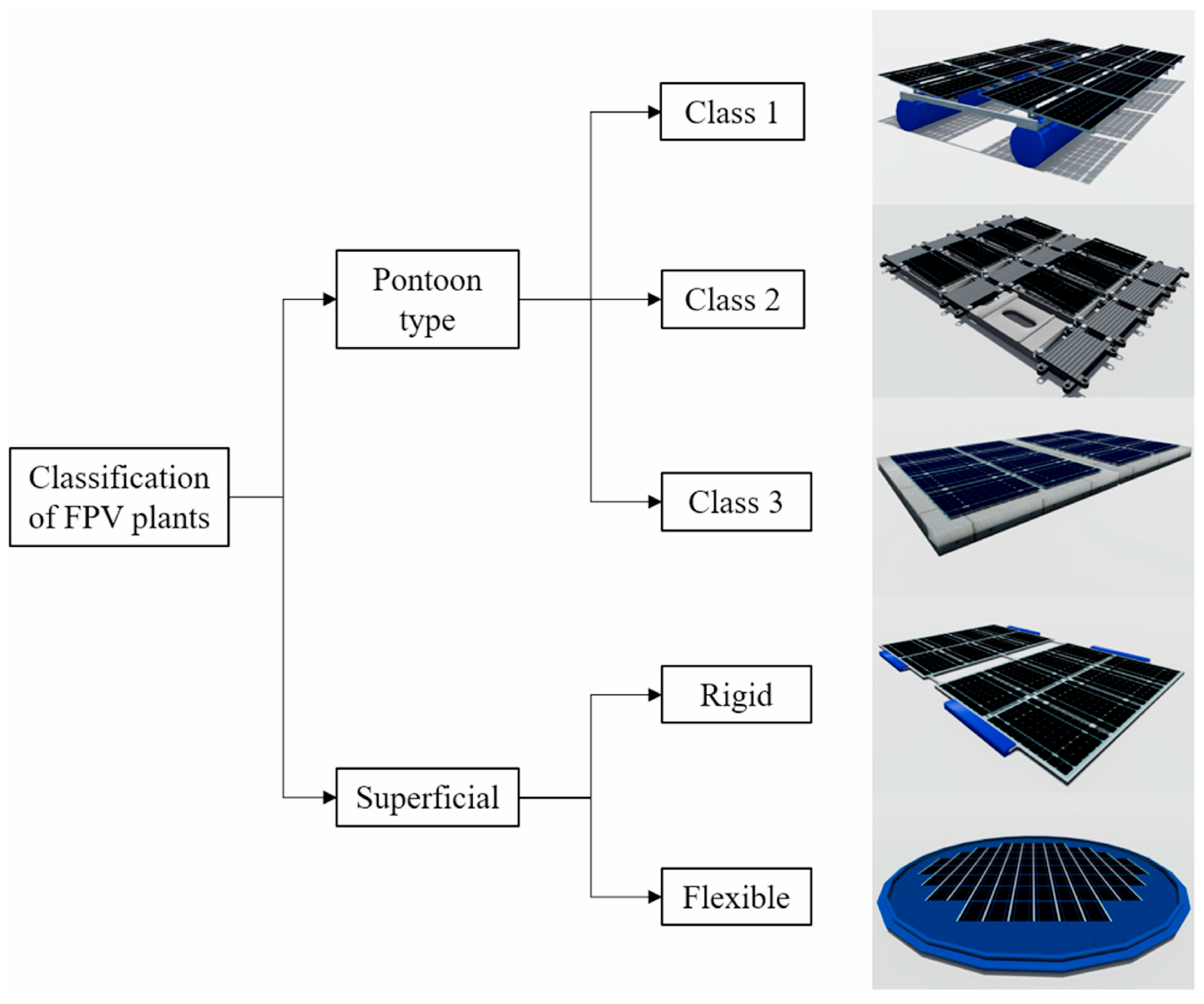
The transition of FPVs to the offshore environment has begun, and many new designs are under investigation to survive the harsh marine environment. Despite the numerous various designs developed, a classification of FPV technologies based on their structural arrangement was attempted in [12], and presented here in Figure 1.

Figure 1.
Classification of FPV systems, from [12].
FPV systems can be superficial, where the PV modules are directly installed over the water surface. Superficial FPV systems can be rigid or flexible. The company, Oceans of Energy, for example, develops an FPV system where groups of solar panels are mounted onto flat rigid floating bodies, interconnected to produce an array. As the solar panels are very close to the free surface, this system can be considered a rigid superficial FPV system. The company installed the first modules of the world’s first offshore FPV farm in the Dutch North Sea. The 500 KWp Oceans of Energy Offshore FPV Farm, now in operation 12 km offshore in high waves since 2020, is said to be developed and proven for offshore high-wave application in salt water, to last 25 years with minimum and safe maintenance. The modular system seems capable to withstand rough sea conditions with maximum wave height up to 13 m [13].
The Norwegian company Sunlit Sea also tested a full-scale model of its superficial rigid floating solar technology [14], made of fully functional solar panel floats, including the proprietary built-in motion sensors, at Stadt Towing Tank hydrodynamic facility in Norway. The model studied comprised solar panel floats linked together. It could only have been tested in frontal wave conditions in this 185 m long and 8 m wide towing tank.
Flexible FPV systems can also use large thin floating flexible films to attach rigid PV panels. This is, for example, the design adopted by the Ocean Sun company, which has installed its circular flexible FPV system on calm waters, and now tests two of those systems close to an offshore wind turbine, making it an hybrid wind–solar offshore system [15].
Thin-film flexible FPVs have been specially developed for the offshore environment [16] and are still in development, for example, in the Solar@Sea and Solar@Sea II projects [17,18]. The Solar@Sea II project includes testing of two floats measuring 7 × 13 m topped by 20 kWp of solar modules, with both the panels and floats made of a flexible material developed by the European consortium. This project is now continued by Bluewater Energy Services, which will build a flexible floating solar demonstration project in the North Sea. The system uses flexible thin-film PV modules and flexible floaters that move with the waves [19].
FPV systems can also be pontoon-type, where an intermediate floating platform holds the rigid PV modules out-of-water. Pontoon-type FPV systems are divided in three classes.
Class 1 pontoon-type FPV systems consist of rafts built with buoyant trusses holding a supporting structure for several PV panels. This is the first design used for the first commercial FPV system, at 175 kWp, installed at the Far Niente vineyard in California [20].
In class 2 pontoon-type FPV systems, individual PV panels are held by a single float with built-in rails, connected to each other through pins. This design was first developed by the French company Ciel et Terre based in Sainghin-en-Mélantois, in 2011 with their patented Hydrelio floating system [21].
In class 3 pontoon-type plants, floats are assembled to create a large floating platform where the PV modules and electrical components are installed independently. These large platforms can then be assembled to create a large power production platform. It is, for example, the design path chosen by SolarDuck company, which tested a scaled model of a 1 MW floating solar platform at the LIR facility in Cork [22]. The scaled model, consisting of thirteen coupled platforms, underwent tests related to induced wave dynamics.
Moss Maritime–Equinor also developed a class 3 FPV plant, consisting of large platforms supporting a large number of PV panels, linked together. They tested their concept using a 1:13 scale model of a floating solar power facility, consisting of 64 floaters, all coupled together [23]. They measured wave information and the movements of floats and loads in the mooring and connection points. Moss Maritime used experimental data to calibrate its numerical model, which will later be used to design and optimise the actual installations for Equinor in a joint floating solar pilot planned for deployment off Frøya in Norway.
Austria’s Swimsol company collaborated with Vienna University of Technology to develop the world’s first offshore floating solar solution, a class 1 pontoon-type FPV system, and they launched in 2014 the world’s first floating solar system, corrosion-proof, that can survive waves of tropical shallow water lagoons, along with currents, tides, extreme UV, and humidity [24]. They actually operate over 15 MWp around the Maldive Islands.
Research is therefore ongoing on this relatively new domain of offshore floating solar farms. Numerical modelling of FPV farms subject to wave forcing have been carried out using different numerical methods, depending on the nature of the system.
Sree et al. developed a numerical method based on finite elements for the design assessment of the maximum stress/strain and displacement of massively connected modular floating solar farms under wave action [25]. They carried out experimental validation of the model using a 1:30 scale model of a global array with 18 walkway modules and 32 PV modules made from flexible perforated sheets in a 0.3 m wide 2D wave flume.
Penpen and Wellen developed a model for large-scale FPVs to be used for flexible FPVs, as developed by the Ocean Sun company, using the Euler–Bernoulli–von Kármán beam model for the structure and nonlinear Stokes theory to model the fluid [26]. They based their theoretical analysis on the problem of floating ice sheets or very large floating structures. Their theoretical model is especially suitable for large membrane-type FPV plants in all water depths.
Numerical simulation is much more difficult for pontoon-type FPV systems. Baruah et al. carried out CFD simulations of a twin-cylinder platform, as used in class I pontoon-type FPV, with the RANS model to take into account the viscous effects [27]. The validity of the viscous model is evaluated for strong nonlinear incident waves through comparisons with experimental data.
Jun-Lee et al. compared experimental and numerical simulations, carried out using CFD model Star-CCM+ V15.06, of a class 1 pontoon-type FPV array composed of an articulated four-unit block, each unit being made of nine square floating blocks supporting a frame holding three rows of solar panels [28]. The mooring conditions simulated a catenary mooring considered at a loosened state at low tide. Experimental tests were carried out in a 3.5 m towing tank at Inha University, India, under frontal and 41° angled regular waves. Numerical results agreed well with experimental data, despite experimental hinges not behaving as the uniaxial numerically simulated hinges.
Ikhennicheu et al. used a quasi-static method to determine environmental loads on a class 2 pontoon-type FPV plant [29]. They considered drag-wind loads, variable depending on the technology and wind direction, current loads, and wave loads with significant wave height derived from the Donelan–Jonswap method. They concluded that the dominant loads for the offshore FPV plant modelled are the wave loads, contrary to the two other FPV plants placed on lakes where wind loads are dominant. They highlight the main challenges in the mooring design for each case, the offshore case requiring the larger number of mooring lines.
Ikhennicheu et al. modelled a 3 × 3 class 2 pontoon-type FPV using the industrial code Orcaflex [30]. They compared different modelling methods, one using the hydrodynamic database (HBD) obtained for one floater for all floaters, i.e., without considering body interactions, one model simulating the whole platform as rigid, and the last one considering all floaters individually, accounting for the hydrodynamic interactions. This last one, being more accurate, is seen as the best approach, and considered as the reference model in the lack of available experimental data. The first modelling strategy gives results close to those of the reference model and is about seven times faster. The model is not yet ready for large-scale islands, and directions are discussed for modelling of large-scale FPV plants.
Accurate numerical modelling of such a class 2 pontoon-type FPV plant is not an easy task. The aim of numerical modelling, in this area, would be to predict the motions, loads, and PV panel production for an entire FPV plant comprising thousands of interconnected modules, under wave, wind, and current loading. CFD models, as that used by Jun-Lee et al. [28], are not yet able not take into account so many individual floaters. There seems to be a lack in the industry for numerical modelling of large pontoon-type FPV plants. A hybrid approach, associating experimental modelling of a subsystem and upscaling using numerical simulations, seems to be the best available approach. Experimental testing is therefore required to appreciate their behaviour under water wave loading, and to obtain solid databases to be used to validate numerical models.
The present paper aims at presenting experimental results on the behaviour of a class 2 pontoon-type FPV array under wave loads. The system studied here is that developed by the company Heliorec. HelioRec is a French company developing class 2 pontoon-type FPV plants destined to be installed nearshore, and later offshore [31,32]. They obtained the support of the four-year Marine Energy Alliance (MEA) European project, aimed at helping marine energy technology companies in early stages of development (TRL 3-4) to progress the technical and commercial maturity of their systems.
As no numerical model is yet able to predict the behaviour of a large array of class 2 pontoon-type FPV plants subjected to water waves, the support offered by MEA to increase the TRL level of HelioRec’s concept included an experimental test campaign, to be carried out in Centrale Nantes’ ocean engineering wave tank.
The experiments described here are destined to give insight into the behaviour of a 4 × 4 class 2 pontoon-type FPV array under wave loads. The experimental results presented here can be used, and are being used, to calibrate and validate numerical models of this class 2 pontoon-type FPV array, notably those developed by HelioRec.
The main contribution of this paper consists in providing a detailed description of the response from the array under wave loads. Particular attention is given to the system’s first resonant mode appearing when the wavelength is twice a floater’s length, which could be an important design case as it implies large loads at the floater connections. Experimental results also show a shadowing effect, implying smaller motions of the back floaters as some wave energy is extracted by the first floaters to see the waves. An important observation is that this shadowing effect seems to occur only for short waves.
This paper first presents the experimental model and experimental setup used in this work, the test conditions, and the experimental procedure. Results on the structure’s behaviour under wave loading are given for the cases of frontal regular waves, frontal irregular waves, oblique regular waves, and oblique irregular waves. Particular attention is given to a specific response from the system observed during the experimental tests.
2. Experimental Modelling
HelioRec’s design belongs to class 2 pontoon-type FPV as it uses individual floaters made of recycled plastic, which reduces both the cost of the system and its carbon footprint, supporting each solar panel. Their array design includes footpath modules, also made of recycled plastic, in order to create catwalks to give human access to individual panels for maintenance. Junctions of the different modules are made using pivot connectors.
2.1. Model Tested
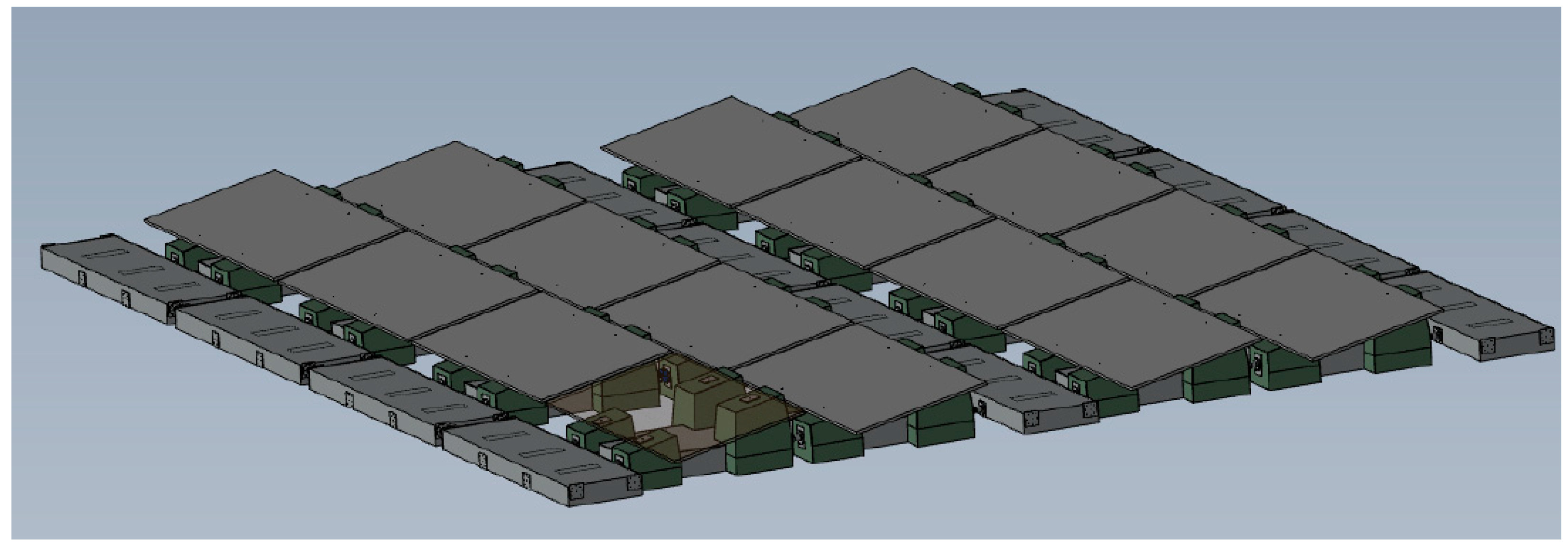
For the experimental tests, part of an array, including 16 solar panel floaters and 12 footpath modules, was designed and built, as shown Figure 2.
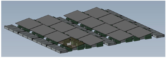
Figure 2.
CAD view of the FPV array tested, with its 16 floaters holding solar panels, and 12 footpath modules forming three catwalks. On the figure, a solar panel has been rendered transparent in order to show the geometry of the floaters.
The aim of the experimental campaign was to gain some valuable experimental data of this system’s response under wave loads to validate numerical modelling of the system, and then later apply this model to achieve accurate simulation of a larger array and finally of an entire FPV plant. Experimental data of interest were the whole system’s response under wave loads, the mooring loads, and loading at the connections in between floaters for design purposes.
For this test campaign, HelioRec wanted to test two different designs of the floats supporting the solar panels. In the first configuration tested, the solar panel floats were empty and open at their bottom. This design would have allowed for stackability of the floats during installation of a large array. In the second design tested, the solar panel floats were closed at 100 mm from the bottom with polystyrene foam.
The target density of the recycled plastic used by the company is low, around 925 kg/m3. The weight of an assembly floater and solar panel was to be 37.35 kg at scale 1, and the weight of the footpath modules 19.4 kg.
With the weight of a module varying with ξ3, ξ being the length scale factor, it was very difficult to technically design a model, rigid enough, with a scale factor larger than 1. This scale was then chosen in order to best approach the main mechanical properties of each module, particularly their mass, the position of their centres of gravity and inertia matrices, and the positions of their connections, and therefore to model at best the whole behaviour of the array. Centrale Nantes’ ocean engineering wave tank, being 30 m wide and 50 m long, could accommodate such a full-scale model of a 4 × 4 solar panel floater array, including its footpaths. The total model was about 8.2 m in width and 7.3 m in length.
All the external faces of the components in the model (footpath and solar panel floats) were made using 3 mm thick aluminium. The footpath modules were waterproof. The panels representing the solar panels were made from plywood, and present on the model in the tests in order to approach at best the target inertia of the assembly floater + panel, and to account for air damping effects of the solar panels on the dynamics of their floats, even if no wind forcing was applied on the structure.
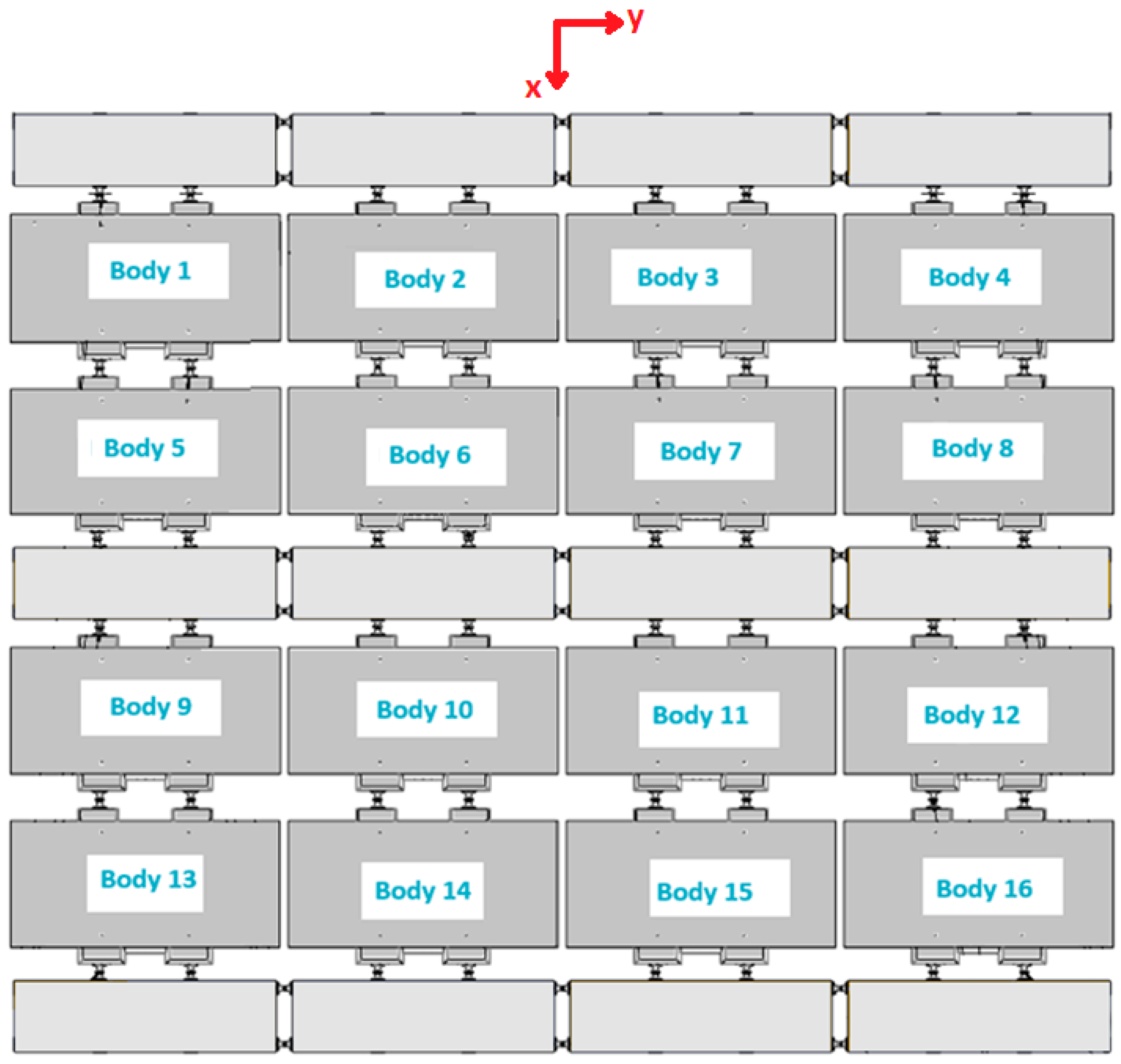
The detailed scheme of the tested array, presented here in Figure 3, best shows the positions of the different pivot connections, around the x-axis between footpath modules, and around the y-axis between footpath modules and the floaters holding solar panels and between the floaters themselves. Figure 3 also presents the numbering of the floaters that is used throughout this paper.
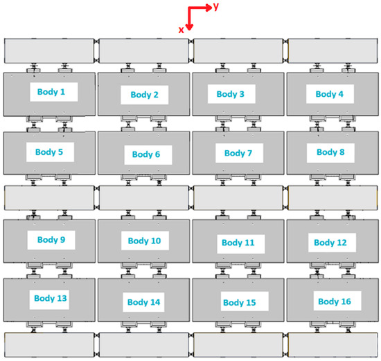
Figure 3.
Top-view scheme of the 4 × 4 solar-panel floating array including the footpath modules represented here in light grey. All connectors, between footpath modules and between floats, were pivot connectors. Frontal incident wave direction is the x-direction.
To obtain information on the loads at the junctions in the array, two six degree-of-freedom (dof) load cells K-MCS10-005 (BG1) from HBM, with measurement ranges for forces Fx and Fy of 1 kN and Fz of 5 kN and for moments Mx, My, and Mz of 50 N.m, were placed on two of the front and back connections of floater number 10, in the centre of the array, as this is where larger loads were predicted by preliminary numerical simulations. These preliminary simulations made by partners of HelioRec were made with a similar array, but with slightly different dimensions as that studied experimentally. The model has not been adapted for the dimensions of the tested array, and no comparisons were made.
The load cells were used principally due to their small size, allowing respecting the geometrical arrangement of the connections between the floaters. These load cells did record loads during the first campaign with the first floaters design, but underwent water damage before the second test campaign with the second floaters design.
The main characteristics of the experimental model investigated here are summarised in Table 1.

Table 1.
Main characteristics of the experimental system under study.
2.2. Test Setup
The tests were carried out in Centrale Nantes’ ocean engineering wave tank, filled with clear water, at about 12 °C during the entire test campaign. As shown in Figure 4, the model front face was placed 13 m away from the wave maker via four horizontal mooring lines, numbered L1 and L2 for the front mooring lines and L3 and L4 for the back mooring lines.
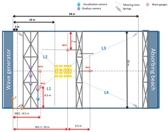
Figure 4.
Top view visualisation of the experimental setup in the wave tank.
Four resistive wave gauges were placed in the tank, WG1 in front of the model, WG2 aligned with WG1 in the y-direction, WG3 on the side of the model, and WG4 behind the model during model testing.
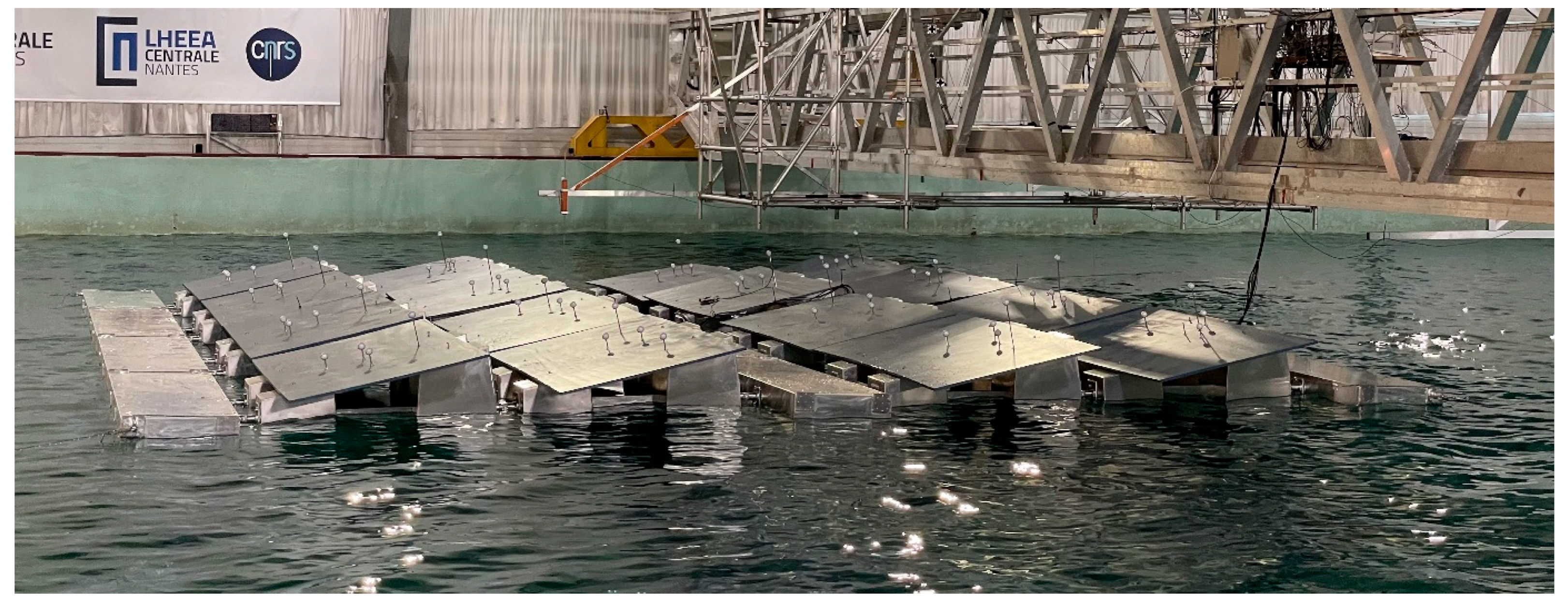
As can be seen on the picture of the array model in still water, presented here in Figure 5, each of the sixteen solar panel modules was equipped with four lightweight markers in order to record their motions using four Qualisys Oqus 7+ aerial motion capture cameras placed on a high footbridge to obtain a large measurement volume.
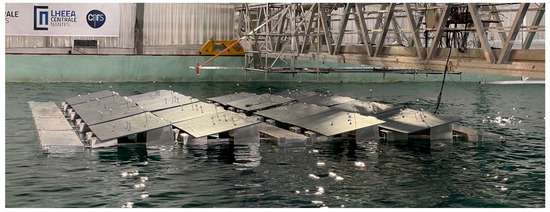
Figure 5.
Side view of the model in water.
The volume area for motion measurement was calibrated according to the Qualysis calibrating procedure, using a fixed L-shaped frame and a wand to be displaced in the large measurement volume. Once calibrated, the system recorded the motion data from the sixteen floaters in MATLAB files (.mat) where the positions of the solar panel floater number i, with i ranging from 1 to 16, were measured and exported as Bodyi_X, Bodyi_Y, and Bodyi_Z in millimetres and its rotations as Bodyi_Roll, Bodyi_Pitch, and Bodyi_Yaw in degrees.
An inertial measurement unit (IMU) Ellipse-E from SBG was fixed on panel number 10, returning its roll, pitch, angular velocities, and accelerations, to confirm video measurements and provide more accurate velocity and acceleration measurements.
All tests were visually recorded using a surveillance camera IP PTZ 360° POE IR 150 M 4 MP Auto-Tracking.
The detailed scheme of the mooring system, presented in Figure 6, shows that the horizontal front mooring lines were at a 44 degree angle from the main model (and basin) direction, and its horizontal rear mooring lines were at a 31 degrees angle. Each line was fixed on a side wall of the tank through a stainless steel spring of stiffness k = 53 (±1) N/m. The length at rest of the springs was 2 m, and pre-tension of about 100 N (±5%) was applied.
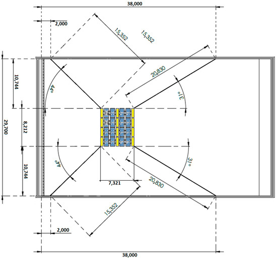
Figure 6.
Detailed arrangement of the mooring setup. All lengths here are given in mm.
The asymmetric arrangement of the mooring lines meant that, at static equilibrium:
with and . The front mooring forces were then larger at equilibrium than the rear mooring forces . Four one dof load cells U9C 500 N from HBM placed at each mooring connection to the footpaths allowed for recording the mooring loads. The mooring forces at static equilibrium were recorded at the start of every test. In most cases and , which correspond to the mooring configuration at equilibrium.
2.3. Test Matrix
The model was tested under regular and irregular wave conditions, with frontal and oblique waves. Table 2 presents the frontal regular waves chosen for the tests, showing their wave height , their period T, and their corresponding wavelength (λ).
Table 2.
Matrix of regular wave conditions used during the tests. Cells in black correspond to non-feasible wave conditions, due to their too large steepness.
Some of these waves were carefully chosen: the 1.27 s waves correspond to a wavelength of 2.45 m, equal to twice a floater’s length, and the 2.15 s waves correspond to a wavelength of 7.26 m, being the total length of the array tested.
The tests with wave parameters highlighted in light grey in Table 2, as that highlighted in dark grey, were also carried out with oblique waves at 15, 30, and 45 degrees. The test highlighted in dark grey was carried out four times during the test campaign to assess the repeatability of the tests.
Tests were also carried out with frontal irregular waves, characterised by Jonswap wave spectra with gamma equal to 3.3. Significant wave heights Hs and peak periods Tp of the wave climates tested are shown in Table 3.
Table 3.
Wave parameters of the irregular wave climates used during the tests.
The wave climates shown in light grey in Table 3 were also carried out in oblique conditions, with incidence angles of 15, 30, 45, and 60 degrees. All waves in oblique conditions were generated by the wave maker using the Dalrymple method.
Obviously, at scale 1, the tank could not produce 9 or 13 s waves as encountered in the ocean, even at nearshore sites. The wave climates tested, particularly their periods, are more specific to the wave climate in a large inland lake than to an offshore test site. The results from the present tests, having for their main purpose to assess the system’s behaviour under wave forcing, can still be used to validate a numerical model of the system by performing model-of-the-model comparisons. As will be seen, over the narrow window of periods tested, a specific wavelength is highlighted where the system’s response is more intense.
The wave climates to be used during testing were all calibrated prior to the tests, with the wave tank empty, equipped with seven calibrated resistive wave probes, including one at 20 m from the wave maker, in the centre of the wave tank, where the model was to be placed. Regular and irregular sea states were run and adjusted until the measured wave height (H or Hs) matched the target, within a 5% error margin.
2.4. Experimental Procedure
One typical experimental test starts with the model at equilibrium in calm water. The acquisition of all sensors is then started, in order to measure calm water loads, and the initial positions of the different floaters. The wave maker is started 45 s later to produce the desired sea state, sending a trigger to the different acquisition systems: one uses catman system acquisition for all sensors, working with frequency modulation signals, much less sensitive to the different magnetic fields generated by the various motors in the laboratory (those of the wave maker, for example), and one used to measure the floaters’ instantaneous positions using the Qualysis video acquisition system. The trigger is later used in post-processing to produce one synchronised single data file. At the end of the test, the wave maker stops and the system slowly returns to its original position in still water. The acquisition systems are then stopped simultaneously.
In order to ensure the quality of the recorded data, a preliminary post-processing of the data is then carried out using MATLAB-based software developed by the laboratory, which displays the acquired signals for visual inspection, allows for choosing the time window to be analysed, and carries out basic wave climate analysis, returning, for example, T or Tp and H or Hs measured by the different wave probes at their specific positions.
3. Experimental Results
The first design of the floaters was tested first, but proved to be very unstable, as some of the entrapped air in the floats escaped from the bottom of the floats, especially when experiencing large pitch motions. Results from this first test campaign are not presented in this paper. The second design of the floaters tested seemed to have better seakeeping, and experimental modelling of this design did provide some valuable information on the system’s behaviour under waves loads. Only results from the test campaign with the second floater design are presented thereafter.
3.1. Pitch Response in Frontal Waves
In this configuration with frontal incident waves, the motions and RAOs of the front, middle, or back lines of floaters (respectively, floaters 1 to 4, or 5 to 8, or 9 to 12, or 13 to 16) are similar.
This is illustrated in Figure 7 for the first line of floaters, i.e., floaters 1, 2, 3, and 4, where the pitch responses from these floaters are very similar, with the same shapes and amplitudes. RAOs are plotted against λ/L, λ being the wavelength and L being the length of a floater between its front and back articulations (L = 1.27 m).
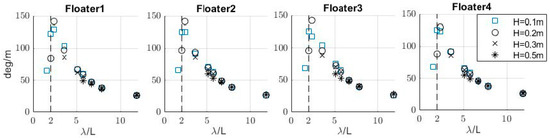
Figure 7.
RAOs of the pitch responses from the front line of floaters (floaters 1 to 4) obtained for frontal regular wave tests.
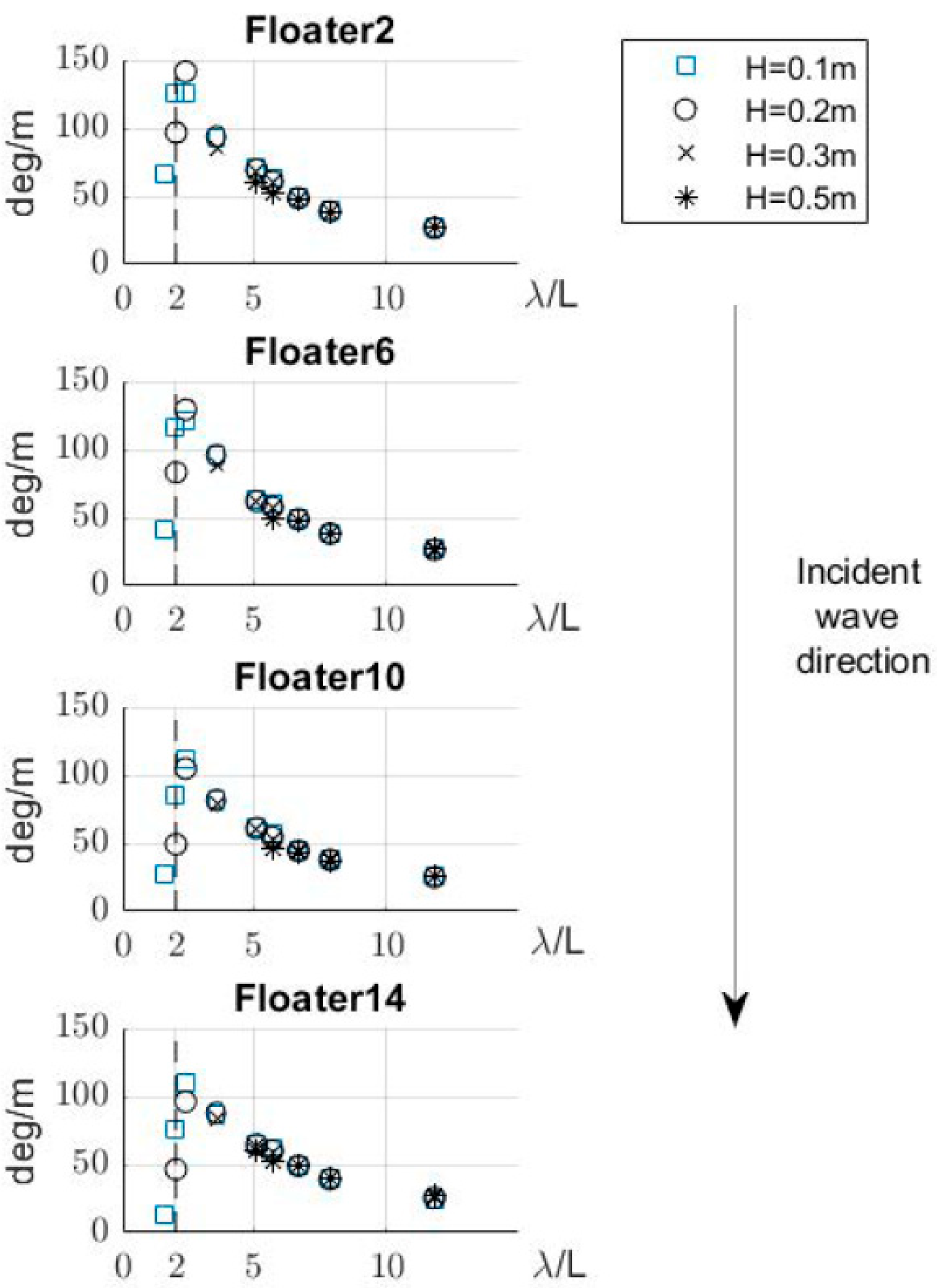
All front floaters present a peak in their pitch response around λ/L = 2, the peak rising to about 150 degrees/m, i.e., about 2.6 rad/m. In the same way, their pitch responses decrease for larger wavelengths. To illustrate how the rest of the array behaves, we present in Figure 8 the RAOs obtained for floaters 2, 6, 10, and 14, each being representative of the line of floaters they belong to.
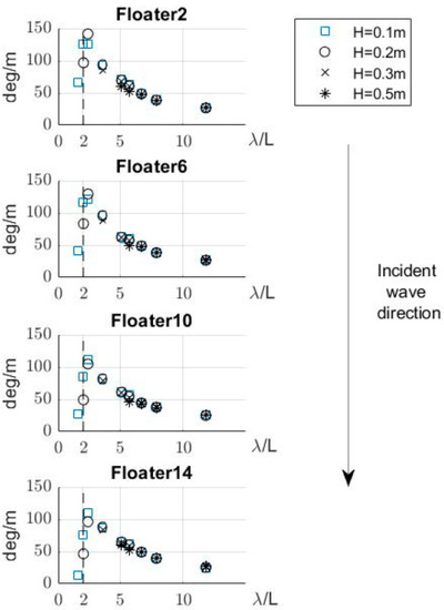
Figure 8.
RAOs of the pitch of floaters 2, 6, 10, and 14 obtained from all regular wave tests.
Figure 8 illustrates that the RAOs of the pitch motions of the floaters do all exhibit a peak when the wavelength is about twice a floater’s length. This peak corresponds to a resonance mechanism due to a natural frequency in the pitch of the assembled system being excited around that wavelength. The RAOs do not change much with the wave amplitude increasing, i.e., with the wave nonlinearity varying. This seems to be a first-order response from the system around this specific wave frequency.
At λ/L = 2, with frontal incoming waves, one row of floaters can be on the ascending part of the wave while the following row is in the descending part of the wave. As can be seen in the plot of the pitch of floaters 1 and 5, presented in Figure 9, the pitch motions of two successive rows are very close to a 180-degree phase shift, for λ/L = 2.
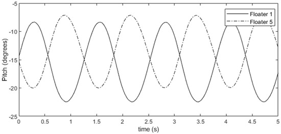
Figure 9.
Pitch time series for floaters 1 and 5 at λ/L = 2, showing out–of–phase pitch motions of the two consecutive rows of floaters, recorded during test 151 with T = 1.27 s and H = 0.2 m.
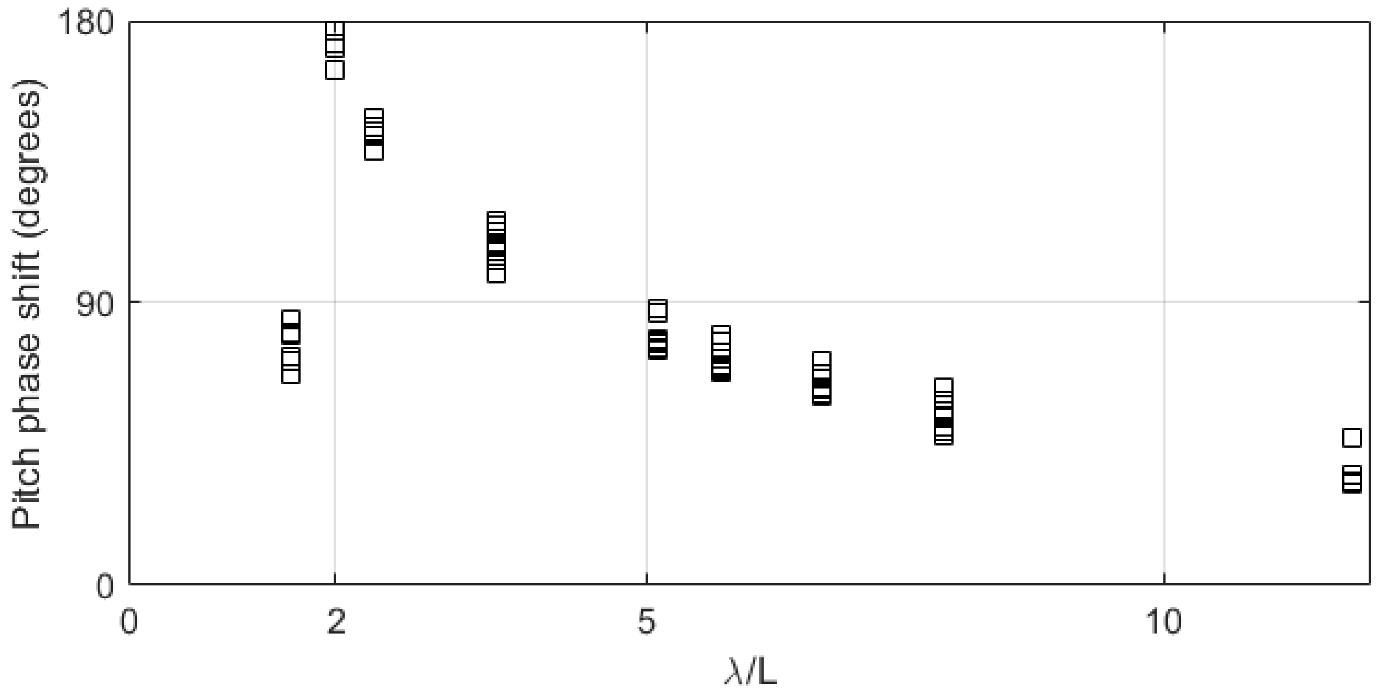
The phase shifts between the pitch motions of all successive floaters (between floaters 1 and 5, 2 and 6, 9 and 13, etc.) are presented in Figure 10. This plot clearly shows nearly 180-degree shifts in the pitch of successive rows of floaters at λ/L = 2, while the phase shifts are much lower for other wavelengths.
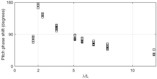
Figure 10.
Pitch phase shifts between the different floaters in each row, obtained from regular wave tests with H = 0.1 m.
Such a pitch response was noted by Jun-Hee at al. [28] for a class 1 pontoon-type FPV articulated system, with pitch RAOs for their articulated floating system showing a large pitch response at wavelengths around twice their body length. Similar pitch response is also observed in the numerical simulations obtained for the class 2 pontoon-type FPD array studied in [30].
This is a response that is very specific to the articulated nature of the system, and the geometrical arrangement of the connections between its bodies. This is a global reaction of the model at this wavelength, highlighted here over this rather narrow wave frequency spectrum experimentally achievable.
This is an important design condition, as loads at the junctions between modules become larger at this frequency. This was observed during testing of the first design of the floaters, which also exhibited an amplified pitch response at λ/L = 2, as shown in Figure 11.
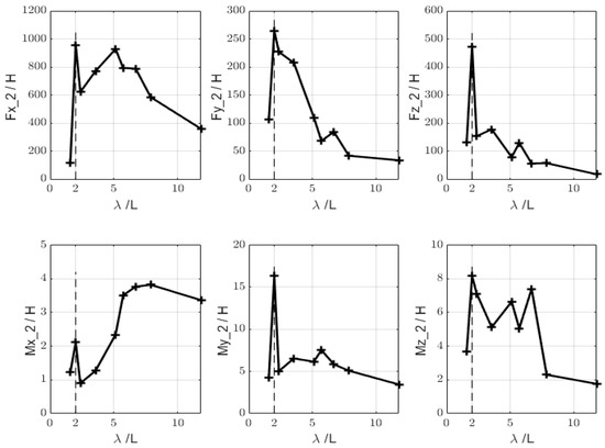
Figure 11.
RAOs of loads measured by load cell number 2, located between floater 10 and floater 14, measured during regular wave tests, with H = 0.1 m, during the first test session with the first floaters design.
Figure 8 also shows an interesting phenomenon. For small values of λ/L, up to about λ/L = 5, the amplitudes of the pitch motions of the floaters in-line with wave direction decrease in the array. Front floaters exhibit larger pitch motions than the floaters behind them, and so on. There seems to be a shadowing effect. The first floaters would appear to extract some energy from the incoming waves, leading to smaller motions of the downward floaters. This would seem to support the hypothesis stated in the conclusions of [30], in which they expect a large array to present negligible motions of the floaters in the centre of the array due to wave energy absorption by side modules. However, this shadowing effect seems to be effective only for small wavelengths, and floaters in the centre of a large array could still be exhibiting long period motions.
Irregular sea states do contain energy over a range of wavelengths, at different amplitudes. Tests carried out in irregular sea states can therefore be analysed to obtain results about the system’s behaviour over the ranges of wavelengths where energy was sent during those tests.
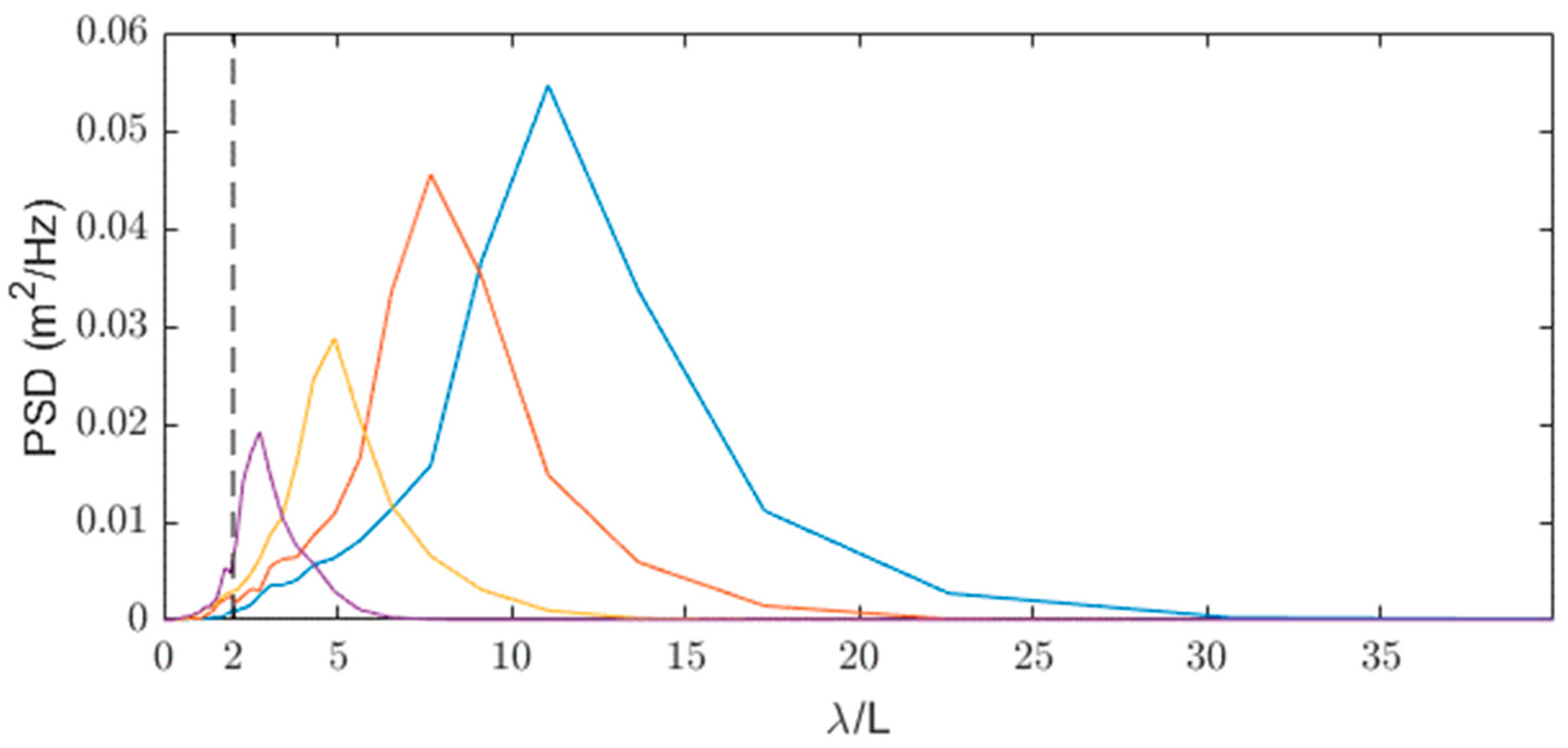
Transfer function estimates are obtained by dividing the spectral density estimates of the considered motion by that of the incoming waves. Transfer function estimates are kept if the coherence between the wave and motion signals is larger than a coherence threshold, usually taken at around 0.9. However, with such a large coherence threshold, the peak response in pitch of the system at λ/L = 2 does not appear in the derived RAOs. This is because little wave energy has been sent at this frequency during the irregular wave tests used, as shown by the Power Spectral Densities (PSD) of the frontal irregular wave climates used, as presented in Figure 12.
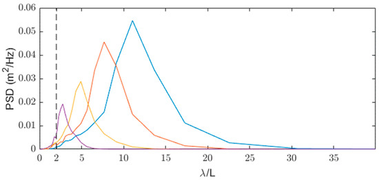
Figure 12.
PSD of the frontal irregular wave climates used during the tests, for cases with Hs = 0.3 m. The different colours will be used to later present results for those conditions.
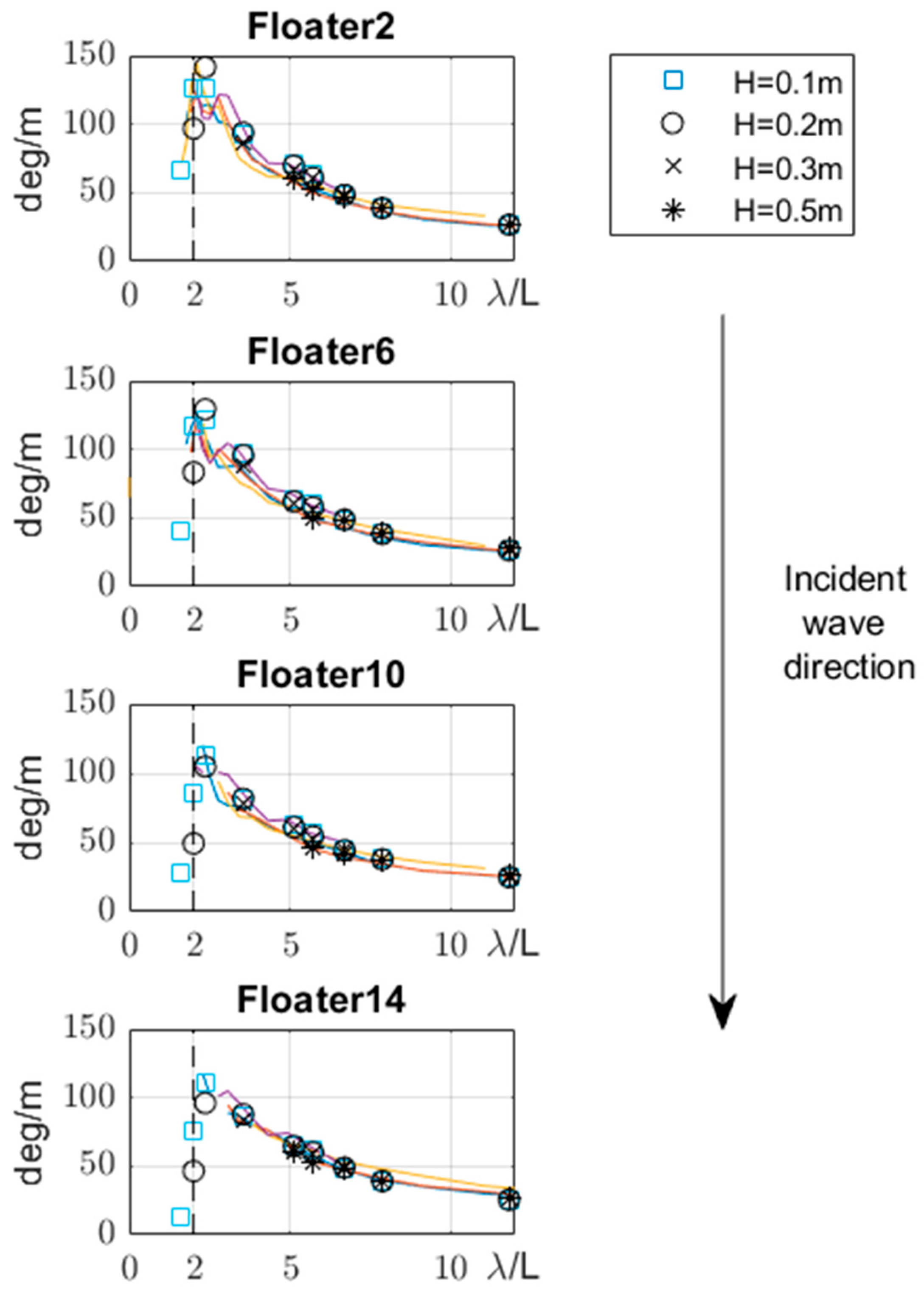
By lowering the coherence threshold to 0.5, the derived RAOs, shown as plain lines in Figure 13 for floaters 2, 6, 10, and 14 with results from regular sea states already presented in Figure 8, do exhibit values for small wavelengths, showing a peak in the pitch response for the front row of floaters at λ/L = 2.
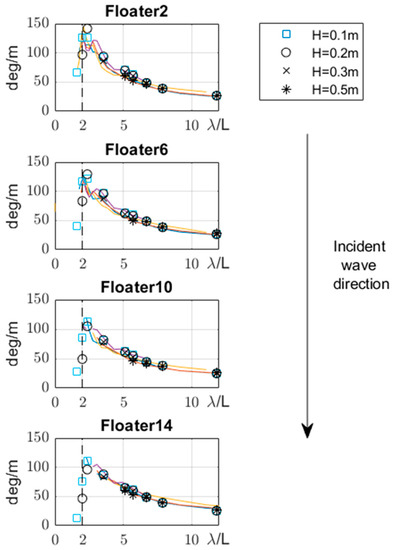
Figure 13.
Pitch RAOs of floaters 2, 6, 10, and 14. Individual markers from experimental data from regular wave tests, and derived RAOs from irregular wave tests in continuous lines, obtained with a coherence threshold of 0.5. The colours used for the derived RAOs correspond to those obtained for wave conditions corresponding to the wave spectra presented in Figure 12.
The spectral analysis carried out shows well the peak in pitch response on floater 2 (it is the same for floaters 1, 3, and 4), facing directly the incoming waves. For the other floaters, the coherence of the wave and motion signals is too low to obtain RAO values for small wavelengths from the frontal irregular wave test runs.
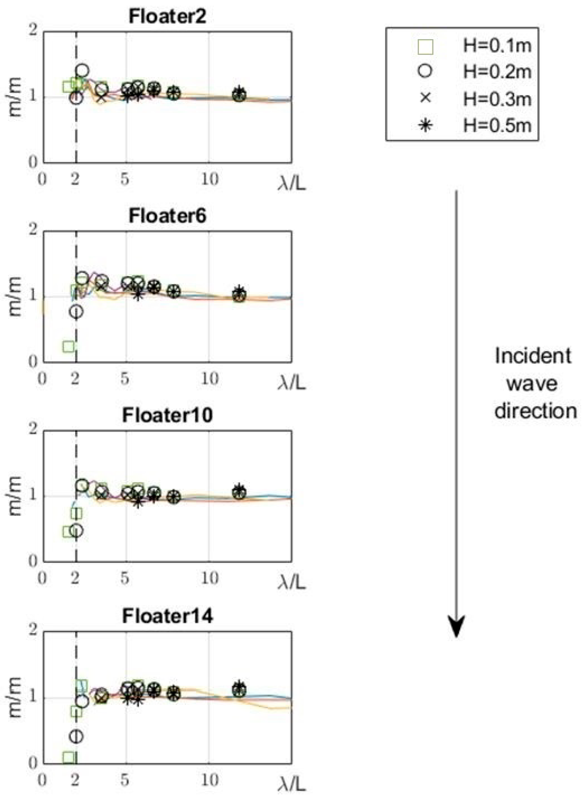
The heave response from the system is presented in Figure 14, again for floaters 2, 6, 10, and 14, as they are the same for other floaters of their corresponding lines for these cases with frontal incoming waves.
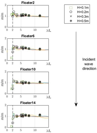
Figure 14.
Heave RAOs of the different floaters, plotted with individual markers for frontal regular wave tests, and in plain lines for the derived RAOs from frontal irregular wave tests. The colours used for the derived RAOs correspond to those obtained for wave conditions corresponding to the wave spectra presented in Figure 12.
Figure 14 shows the system exhibiting heave RAOs at around 1 m/m for the front row floaters at λ/L = 2, showing that the front row of floaters rides the waves. The heave response from the next rows of floaters decreases at this frequency. The whole system’s amplified pitch motion at this frequency seems to limit the heave motion of the rear floaters.
The heave RAOs of the front rows of floaters peak around λ/L = 2.36, at about 1.2, and then decrease to tend towards 1 with the wavelength increasing. Similar heave RAOs are presented in [30].
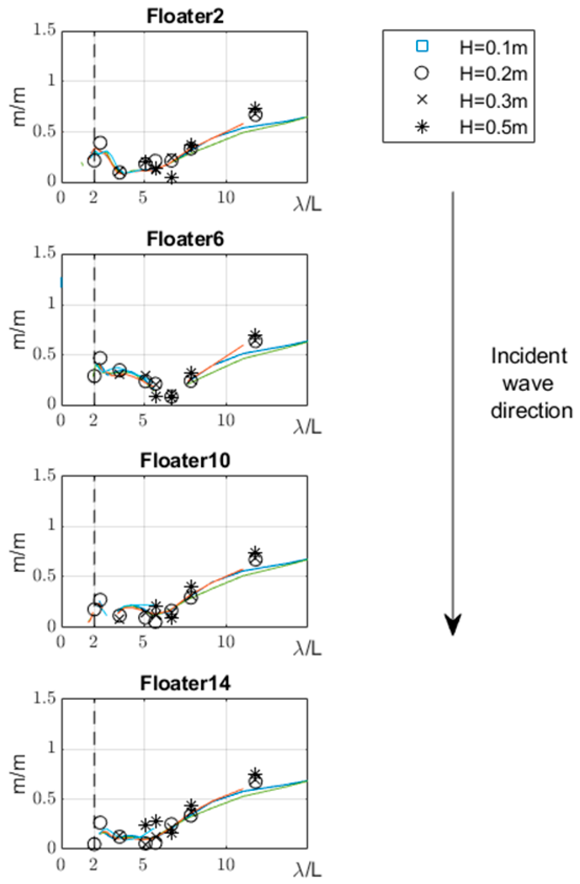
The system exhibits small surge displacements for small wavelengths, as shown by the surge RAOs of the different floaters, as presented in Figure 15. It shows a small peak response at λ/L = 2.36, but from λ/L > 3, the surge of the system increases with the wavelength. Since the floaters are all linked together, the surge motion (and RAOs) of each floater in frontal waves is very similar.
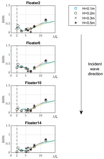
Figure 15.
Surge RAOs of the different floaters, plotted with individual markers for frontal regular wave tests, and in plain line for the derived RAOs from frontal irregular wave tests. The colours used for the derived RAOs correspond to those obtained for wave conditions corresponding to the wave spectra presented in Figure 12.
3.2. Repeatability of Tests
As mentioned in Section 2.2, the test with frontal regular waves characterised by T = 1.69 s and H = 0.2 m was carried out four times during the test campaign to assess the repeatability of the tests.
Root-Mean Squared (RMS) values of the pitch and heave responses from all floaters are presented in Figure 16, divided by their values for test number 149.
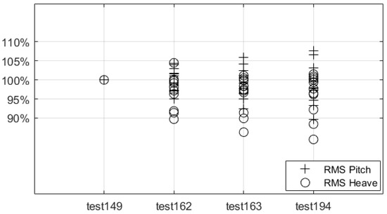
Figure 16.
Differences in RMS values of the pitch and heave responses from all floaters compared to their response in test number 149.
It can be seen that the RMS values of the pitch and heave responses from nearly all floaters stay within 90% and 110% of the value measured in test number 149. The repeatability of the tests is then asserted to give results within a 10% error margin. This relatively large error margin can be explained by the complex nature of the articulated system studied, which renders it quite sensitive to initial conditions. Test number 194, where the largest discrepancies were measured, was also run after a test with frontal irregular wave conditions. The time for the wave tank to come back to calm water conditions after such a test was certainly long, and test number 194 was certainly started in the tank still containing some water motion. Discrepancies are noted in the system, which is sensitive to initial conditions.
3.3. Effect of Wave Incidence Direction
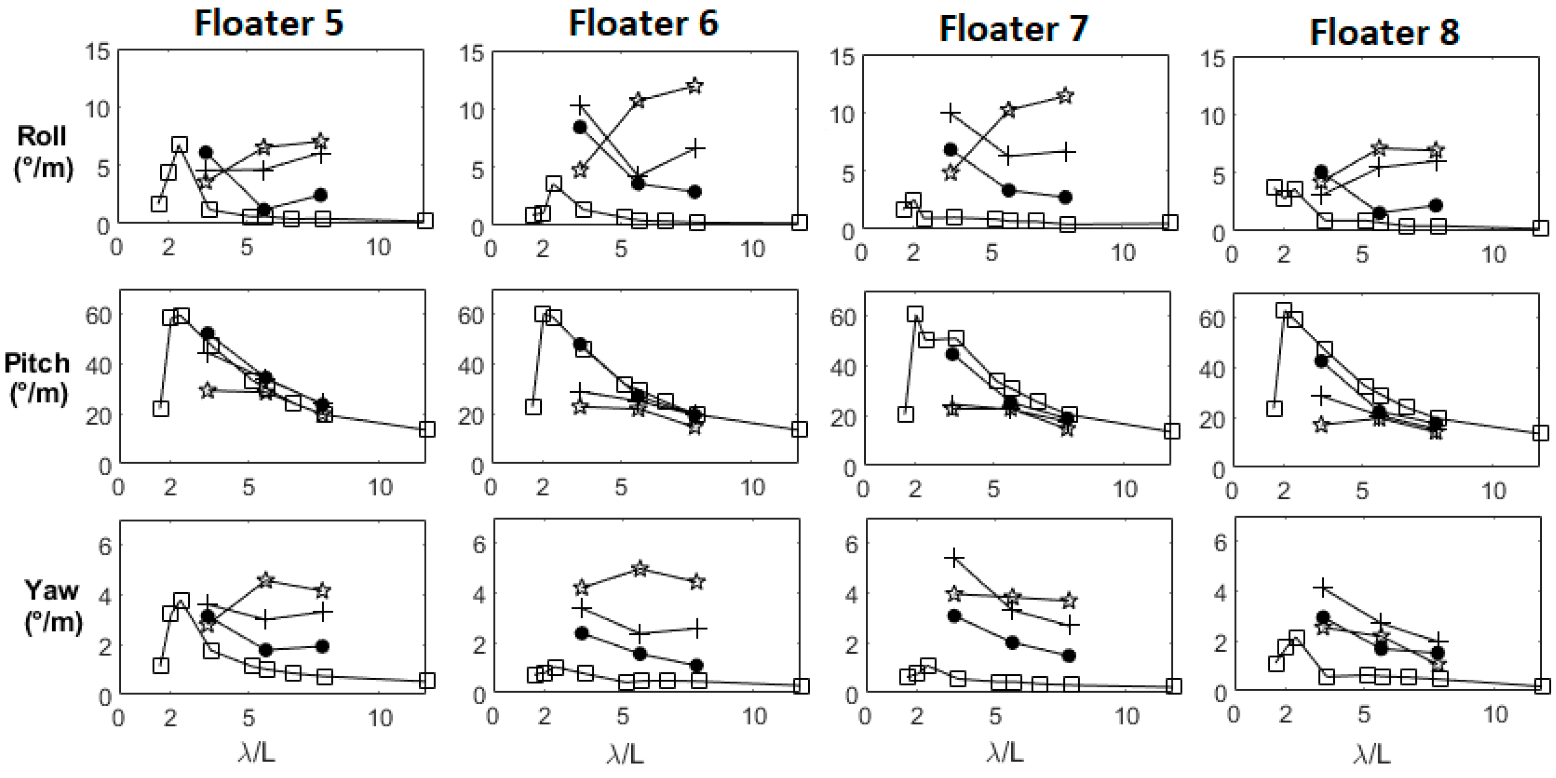
Some tests were run with the wave incident direction at 15, 30, and 45 degrees. RAOs obtained from tests run with oblique regular waves, presented in Figure 17 for the second line of floaters (floaters 5 to 9), show that, for long wavelengths, the roll and yaw motions were becoming more excited with increasing wave direction.
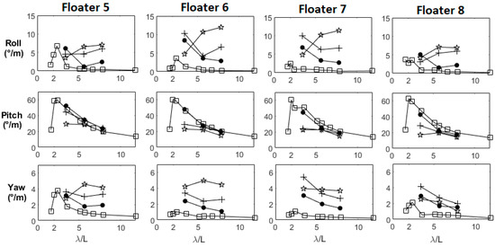
Figure 17.
RAOs in roll, pitch, and yaw of the second line of solar panels (floaters 5 to 8) in frontal (□) and oblique regular waves (● for 15° angled waves, + for 30°, ☆ for 45°), with H = 0.1 m.
The pitch motion was observed to decrease slightly compared to the case with frontal waves. It can also be observed that the roll and yaw motions are lower for angled waves for body number 8 than for the other bodies. The incident angled waves coming from the other side of the model (here on the side of floater number 5), this floater on the other side of the model seems somewhat protected by the shadowing effect of the other floaters.
4. Conclusions
Scale 1 model testing of a 4 × 4 array of floating solar panels was carried out in Centrale Nantes’ ocean wave engineering tank. The model tested was a 1:1 scale of a system of 4 × 4 floaters holding solar panels, with three rows of floating footpaths designed for maintenance. The total model, encompassing 16 solar panel modules and 12 footpaths, was about 8.2 m in width and 7.3 m in length. The rigidity of the model was a key design factor, as its connections on the flat faces of different parts were to be rigid. Rigid model design of the floaters and footpaths with very low density was achieved using 3 mm thick aluminium rigid plates and lightweight foam. This allowed for the introduction of two load cells onto one of the model’s modules, which returned interesting results in an initial campaign. Sadly, the loads cells were damaged by water during the tests and load measurements are missing for the last part of the test campaign, including the testing of model design number two, whose results are presented in this paper.
Tests were carried out with regular and irregular frontal and oblique incoming waves.
At that scale, the tank could produce waves from 1 up to 3.5 s, which is more representative of a large inland lake wave climate than real offshore sea conditions.
Nevertheless, the tests allowed for isolating one particular phenomenon, a first-order pitch resonant mode excitation of the multibody articulated system, when wavelengths are about twice the floater’s length. This could be an important point for design as loads at the floater connections are larger at that frequency.
Further work needs to be carried out now to assess the system’s behaviour in a nearshore or offshore site. A suitable numerical model is necessary to perform a model-of-the-model and adjust the numerical model. This one could later be used for simulating the array behaviour under a wider wave spectrum, with characteristic wave periods of a nearshore site, and would be aimed at simulating the response from a large array.
For the moment, CFD and SPH modelling of the tests presented here is being attempted by HelioRec. CFD or SPH simulations of such an array with 28 interconnected floating bodies under wave loads will require a very long time. A suitable numerical method for modelling a large array of class 2 pontoon-type FPV plants comprising thousands of modules seems to be lacking for safe development of the industry.
Author Contributions
Design, coordination, and supervision of experimental tests, and post-processing: S.D. Post-processing and writing—original draft preparation: S.B. Project administration, test campaign specification, and funding acquisition: T.S. Reviewing and editing: H.E. Test campaign requirements and scale model funding: P.V. All authors have read and agreed to the published version of the manuscript.
Funding
This research was funded by the Marine Energy Alliance European program. The Marine Energy Alliance (MEA) is a 4-year transnational European Territorial Cooperation project running from May 2018 to May 2022. MEA received ERDF support totalling EUR 3.6 million through the INTERREG North West Europe program.
Data Availability Statement
The data are not publicly available due to confidentiality reasons.
Acknowledgments
Centrale Nantes acknowledges the provision of test data from HelioRec for analysis.
Conflicts of Interest
The authors declare no conflict of interest.
References
- U.S. Energy Information Administration. International Energy Outlook 2021. 2021. Available online: https://www.eia.gov/outlooks/ieo/tables_side_xls.php (accessed on 14 November 2022).
- SolarPower Europe. Global Market Outlook for Solar Power 2022–2026. 2022. Available online: https://www.solarpowereurope.org/insights/market-outlooks/global-market-outlook-for-solar-power-2022 (accessed on 9 December 2022).
- Oliveira-Pinbto, S.; Stokkermans, J. Assessment of the potential of different floating solar technologies—Overview and analysis of different case studies. Energy Convers. Manag. 2020, 211, 112747. [Google Scholar] [CrossRef]
- Bellini, E. South Korean Government Announces 2.1 GW Floating PV Project. 19 July 2019. Available online: https://www.pv-magazine.com/2019/07/19/south-korean-government-announces-2-1-gw-floating-pv-project/ (accessed on 21 November 2022).
- Rosa-Clot, M.; Tina, G. Current status of FPV and trends. In Floating PV Plants; Academic Press: Cambridge, MA, USA, 2020; pp. 9–18. [Google Scholar]
- Solar Edition. Cumulative FPV Capacity Scales up to 2 Times in Less than Two Years. 30 October 2020. Available online: https://solaredition.com/cumulative-fpv-capacity-scales-up-to-2-times-in-less-than-two-years/ (accessed on 6 March 2023).
- Hasnain, Y.E.; Khokhar, M.Q.; Zahid, M.A.; Kim, J.; Kim, Y.; Cho, E.; Cho, Y.H.; Yi, J. A Review on Floating Photovoltaic Technology (FPVT). Curr. Photovolt. Res. 2020, 8, 67–78. [Google Scholar]
- DNV. DNV-RP-0584: Design, Development and Operation of Floating Solar Photovoltaic Systems. 2021. Available online: https://www.dnv.com/energy/standards-guidelines/dnv-rp-0584-design-development-and-operation-of-floating-solar-photovoltaic-systems.html (accessed on 7 December 2022).
- Kichou, S.; Skandalos, N.; Wolf, P. Floating photovoltaics performance simulation approach. Heliyon 2022, 8, e11896. [Google Scholar] [CrossRef]
- Liu, H.; Krishna, V.; Leung, J.L.; Reindl, T.; Zhao, L. Field experience and performance analysis of floating PV technologies in the tropics. Prog. Photovolt. Res. Appl. 2018, 26, 957–967. [Google Scholar] [CrossRef]
- Oliveira-Pinto, S.; Stokkermans, J. Marine floating solar plants: An overview of potential, challenges and feasibility. Proc. Inst. Civ. Eng.—Marit. Eng. 2020, 173, 120–135. [Google Scholar] [CrossRef]
- Claus, R.; López, M. Key issues in the design of floating photovoltaic structures for the marine environment. Renew. Sustain. Energy Rev. 2022, 164, 112502. [Google Scholar] [CrossRef]
- Oceans of Energy. Available online: https://oceansofenergy.blue/technology/ (accessed on 10 October 2022).
- Sun, O. Haiyang (Offshore). Available online: https://oceansun.no/project/haiyang-offshore/ (accessed on 30 January 2023).
- Trapani, K.; Millar, D.L. The thin film flexible floating PV (T3F-PV) array: The concept and development of the prototype. Renew. Energy 2014, 71, 43–50. [Google Scholar] [CrossRef]
- Solliance Solar@Sea Starts Testing Floating Solar System. Available online: https://www.solliance.eu/2018/solaratsea-starts-testing-floating-solar-system/ (accessed on 5 December 2022).
- Scully, J. Researchers Trial Thin-Film Floating Solar System for Offshore Applications. 29 November 2021. Available online: https://www.pv-tech.org/researchers-trial-thin-film-floating-solar-system-for-offshore-applications/ (accessed on 6 December 2022).
- Santos, B. Dutch Developer Secures Funds for Flexible Floating Solar Pilot in North Sea. 2 December 2022. Available online: https://www.pv-magazine.com/2022/12/02/dutch-developer-secures-funds-for-flexible-floating-solar-pilot-in-north-sea/ (accessed on 12 December 2022).
- Sujay, S.P.; Wagh, M.; Shinde, N. A review on floating solar photovoltaic power plants. Int. J. Sci. Eng. Res. 2017, 8, 789–794. [Google Scholar]
- Ciel et Terre Hydrelio®: The Patented Floating PV System. Available online: https://beta.ciel-et-terre.net/hydrelio-technology/our-hydrelio-solutions/ (accessed on 10 November 2022).
- Garanovic, A. SolarDuck’s Offshore Floating Solar Array Aces LiR NOTF Tests. August 2022. Available online: https://www.offshore-energy.biz/solarducks-offshore-floating-solar-array-aces-lir-notf-tests/ (accessed on 15 December 2022).
- Garanovic, A. Sintef Ocean on Point for Moss Maritime-Equinor Floating Solar Model Trials. 5 May 2021. Available online: https://www.offshore-energy.biz/sintef-ocean-on-point-for-moss-maritime-equinor-floating-solar-model/ (accessed on 15 December 2022).
- Swiwsol. Available online: https://swimsol.com/#lagoon (accessed on 15 November 2022).
- Garanovic, A. Sunlit Sea Starts Floating Solar Wave Tank Trials. 23 March 2022. Available online: https://www.offshore-energy.biz/sunlit-sea-starts-floating-solar-wave-tank-trials/ (accessed on 10 October 2022).
- Sree, D.K.; Law, A.W.-K.; Pang, D.S.C.; Tan, S.T.; Wang, C.L.; Kew, J.H.; Seow, W.K.; Lim, V.H. Fluid-structural analysis of modular floating solar farms under wave motion. Sol. Energy 2022, 233, 161–181. [Google Scholar] [CrossRef]
- Pengpeng, X.; Wellens, P.R. Fully nonlinear hydroelastic modeling and analytic solution of large-scale floating photovoltaics in waves. J. Fluids Struct. 2022, 109, 103446. [Google Scholar]
- Baruah, G.; Karimirad, M.; Abbasnia, A.; MacKinnon, P.; Sarmah, N.; Moghtadaei, A. Numerical Simulation of Nonlinear Wave Interaction with Floating Solar Platforms with Double Tubular Floaters Using Viscous Flow Model. In Proceedings of the 41st International Conference on Ocean, Offshore and Arctic Engineering, Hamburg, Germany, 5–10 June 2022. [Google Scholar]
- Jun-Hee, L.; Kwang-Jun, P.; Soon-Hyun, L.; Hwangbo, J.; Tae-Hyu, H. Experimental and Numerical Study on the Characteristics of Motion and Load for a Floating Solar Power Farm under Regular Waves. J. Mar. Sci. Eng. 2022, 10, 565. [Google Scholar] [CrossRef]
- Ikhennicheu, M.; Dangale, B.; Pascal, R.; Arramounet, V.; Trebaol, Q.; Gorintin, F. Analytical method for loads determination on floating solar farms in three typical environments. Sol. Energy 2021, 219, 34–41. [Google Scholar] [CrossRef]
- Ikhennicheu, M.; Blanc, A.; Danglade, B.; Gilloteaux, J.-C. OrcaFlex Modelling of a Multi-Body Floating Solar Island Subjected to Waves. Energies 2022, 15, 9260. [Google Scholar] [CrossRef]
- Centrale Nantes. Available online: https://lheea.ec-nantes.fr/test-facilities/ocean-tanks/hydrodynamic-and-ocean-engineering-tank (accessed on 3 October 2022).
- Heliorec. Available online: https://www.heliorec.com/tech (accessed on 3 October 2022).


Disclaimer/Publisher’s Note: The statements, opinions and data contained in all publications are solely those of the individual author(s) and contributor(s) and not of MDPI and/or the editor(s). MDPI and/or the editor(s) disclaim responsibility for any injury to people or property resulting from any ideas, methods, instructions or products referred to in the content. |
© 2023 by the authors. Licensee MDPI, Basel, Switzerland. This article is an open access article distributed under the terms and conditions of the Creative Commons Attribution (CC BY) license (https://creativecommons.org/licenses/by/4.0/).