Abstract
This study focuses on optimizing the lifetime and cost of an electric vehicle powertrain by optimizing the motor’s geometrical parameters and the bus voltage while considering the battery’s sizing. We employ the WLTP driving cycle to evaluate the powertrain’s performance and use finite element and analytical modeling to consider electromagnetic, thermal, and aging behaviors. Our research investigates the interplay between the battery and motor, exploring how varying the motor geometry and parameters affects the powertrain’s overall lifetime and cost. Our findings will contribute to developing more efficient and cost-effective electric powertrains.
1. Introduction
The shift toward electric vehicles (EVs) has become increasingly popular in recent years due to the need to reduce carbon emissions and combat climate change [1,2]. One of the key components of an EV powertrain is the electric motor, which converts electrical energy stored in the battery into mechanical energy to propel the vehicle [3]. The motor plays a critical role in determining the overall efficiency, range, and cost of an EV, making it crucial to carefully consider the selection and optimization of the motor technology [4,5].
However, with so many motor technologies available in the market, it can be challenging to choose the optimal one that meets the specific requirements of an EV powertrain [6]. Additionally, testing different motor designs can be expensive and time-consuming, making the use of simulations a more practical and cost-effective solution [7]. Nevertheless, creating accurate and reliable simulations that capture all the relevant phenomena and complexities of motor operation remains a significant challenge [8].
Accurate simulations must be compared against experimental results to ensure their reliability. However, multiple factors must be considered for accurately modeling a motor, such as the electromagnetic field, thermal behavior, and aging characteristics, among others. Building high-fidelity models that consider all these aspects can be time-consuming, especially when running optimization studies [9].
Moreover, to achieve the best performance and efficiency in motor optimization, other powertrain components, such as the battery, must be considered. Thus, selecting the optimal motor topology [10], technology, and bus voltage value requires a comprehensive analysis that takes into account multiple factors to achieve the best balance between lifetime, cost, and performance [7,11].
To achieve this goal, this study will use Ansys Electrotronics 2022 R2 [12] for modeling the electromagnetic part of the motor, Motor CAD [13] for modeling the thermal part, and analytical modeling for the aging behavior, which will take into account both thermal and electromagnetic aspects. By using these three tools together, the study aims to create an accurate and reliable simulation that can be used to optimize the motor design, taking into account all the relevant phenomena and interactions between different powertrain components in addition to the impact of bus voltage variation on the overall optimization convergence as illustrated in Figure 1.
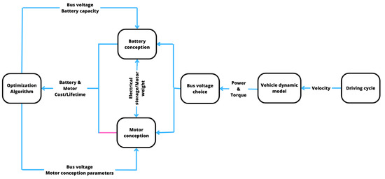
Figure 1.
Work methodology.
Overall, this study aims to provide insights into the optimal design of a synchronous permanent magnet motor (PMSM) for EV powertrains by addressing the challenges associated with accurate modeling and optimization. The study thereby aims to contribute to the development of more efficient, reliable, and cost-effective electric vehicles.
2. Materials and Methods Used in Powertrain Modeling and Optimization
2.1. Motor Characteristics Required for the Automobile Industry
The electric drive is a critical component of an electric vehicle. However, it must have the appropriate speed torque characteristics listed in Figure 2 [5,9,14] with CPSR for constant power speed range. There are two zones in these properties: one with constant torque and one with constant power. When starting, accelerating, or mounting a hill, maximum torque is required, and the motor operates in the region at constant torque. In this zone, the armature voltage varies to modify speed, while the armature and excitation currents remain constant to generate the required torque. At speeds larger than the base speed, the motor runs in the constant power zone [15].
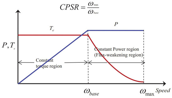
Figure 2.
Required motor characteristics for an automotive application.
In this zone, the velocity is changed by varying the excitation current while the voltage and armature current remain constant at their nominal values. As the excitation current (flow) decreases, the speed increases, resulting in a nearly constant counter-electromotive force and, as a result, essentially constant power [16,17].
Electric vehicles rely on electric motors to produce the necessary torque to turn their wheels. The performance of an electric vehicle largely depends on the motor’s capabilities, which must exhibit a variety of characteristics [18,19]. These characteristics include:
- High power density;
- Consistent high efficiency across a range of speed and torque levels;
- Rapid dynamic response;
- Reliable performance across a range of operating conditions;
- Two operating zones that cover a broad range of speeds, torque, and power; and
- An affordable price point.
Over the years, improvements in high-power converters, advanced control techniques, and high-energy permanent magnet materials have led to substantial enhancements in electric motor performance. As a result, various types of electric motors can now be utilized in electric vehicles, although some are more commonly used than others. In the following subsection, we will examine the most frequently used types of motors.
Comparison of the Main Motors Used in Electric Automotives
Table 1 presents a comparison of the main electric motors used in electric vehicles (EVs). The comparison is based on various factors such as efficiency, speed range, power density, maximum torque, reliability, cost, and maturity of the technology. The five most widely used types of EV motors were selected for comparison, and each factor was rated on a scale of 1 (low) to 5 (high) [5,17]. The table shows that the brushless PM (permanent magnet) and PM SYN (permanent magnet synchronous) motors have the highest overall score of 35 points, indicating that they are the best performers in terms of the considered factors. Both motors score highly in power density, efficiency, reliability, and maturity. However, the PM SYN motor is rated slightly lower in terms of controllability and noise. The induction motor comes in second place, with a score of 35, thanks to its high reliability, controllability, and maintenance ratings. The SR (switched reluctance) motor and PM DC (permanent magnet direct current) motor have a total score of 30 and 25 points, respectively.

Table 1.
Motor technology comparison.
It is worth noting that while the DC motor has a lower overall score than other types, it still has some advantages. For example, it is the most cost-effective and the easiest to maintain. Additionally, it has a high rating for controllability.
Overall, the choice of motor for an EV will depend on various factors such as the intended use, cost considerations, and desired performance characteristics.
2.2. Adopted Specifications for the Study
2.2.1. Characteristics of the Chosen Vehicle
In this study, the dynamic model of a vehicle was based on the parameters of the Bluecar Beloré, an urban electric car. The characteristics of the electric vehicle used in the model are presented in Table 2.
Table 2.
Key Characteristics of the Bluecar Beloré [20].
2.2.2. Characteristics of the Selected Driving Cycles
To compare pollutant emissions and fuel economy of different vehicles on a standardized basis, test cycles with controlled speed and elevation profiles are used. These duty cycles are replicated on roller test benches under controlled conditions to mimic the energy losses of the vehicle during driving. Tests are performed under tightly controlled environmental conditions to ensure consistent and reproducible results, with the vehicle undergoing a thermal conditioning procedure before the test begins.
For this study, only one driving cycle is considered, namely the WLTP (Worldwide Harmonized Light Vehicles Test Procedure). The WLTP cycle illustrated in Figure 3 replaced the previous NEDC standard and has been established using real-world driving data collected globally, unlike the previous cycle, which was based on theoretical speed variations. The WLTP cycle consists of four sections, each with different average speeds to represent diverse driving scenarios such as urban, rural, extra-urban, and motorways [21].
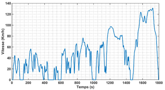
Figure 3.
Driving cycle speed evolution (WLTP).
The choice of the WLTP driving cycle for this study is based on its comprehensive representation of real-world driving conditions and its wide acceptance in the automotive industry. The WLTP driving cycle incorporates a range of driving scenarios and average speeds, providing a realistic evaluation of the motor optimization process. While there are various standard driving cycles available, each with its own characteristics, the WLTP driving cycle offers a robust framework for assessing electric vehicle performance.
It is worth noting that the selection of the driving cycle does have an impact on the motor optimization results. This factor has been acknowledged in previous studies, particularly in [22,23].
2.2.3. Characteristics of the Selected Battery Technologies
For our study, we will focus on batteries that utilize NMC Li-ion technology. The electrical characteristics and parameters of this battery type are presented in Table 3.
Table 3.
Electrical characteristics of NMC Li-ion battery [24].
2.2.4. Selected Electric Motor Technology
The permanent magnet synchronous motor (PMSM) was chosen for our study because of its durability, low maintenance, and high performance across a wide operating range. More specifically, the motor geometry of the well-known Toyota Prius hybrid vehicle was chosen illustrated in Figure 4.
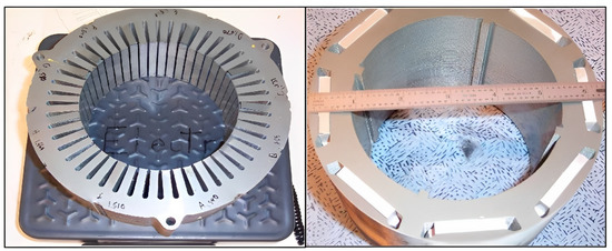
Figure 4.
Toyota Prius PM synchronous motor.
2.3. Electric Powertrain Modeling
2.3.1. Vehicle Dynamic Model
The utilization of the vehicle dynamic model enables estimation of the torque, power, velocity, and energy requirements (Figure 5) for a given driving cycle, and these parameters can be utilized to determine the appropriate specifications and sizing for the battery and electric motor.
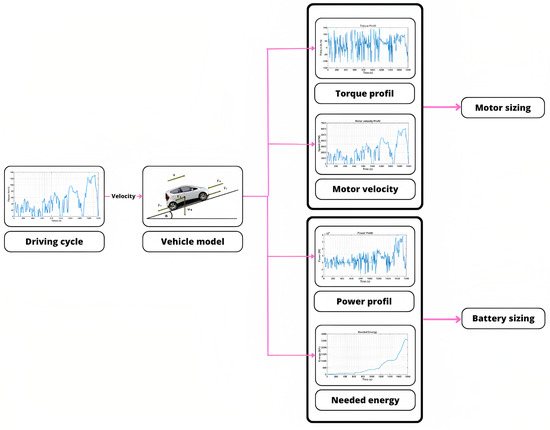
Figure 5.
Estimating driving cycle power/torque and energy.
The energy generated by the powertrain of a vehicle is stored within the vehicle. Nevertheless, the stored energy can be consumed by different resistant forces. Energy can be stored in various forms:
- Kinetic energy is stored during acceleration.
- Potential energy is stored when the vehicle reaches altitudes higher than the reference level.
The mechanical energy “consumed” during vehicle operation is dependent on three main factors:
- The effect of aerodynamic friction
- The effect of rolling friction
- The energy lost during braking
- represents the velocity of the vehicle.
- represents the total energy consumed by the vehicle during a complete cycle.
- represents the power required at time t to overcome the forces that affect the vehicle’s mechanical energy consumption.
- Wanteddistance represents the desired autonomy.
The forces that affect the vehicle’s mechanical energy consumption while driving include aerodynamic friction, rolling friction, gravity-induced force on non-horizontal roads, and other unaccounted effects, which are all grouped as Fd. Another factor is the propulsive force, which is the difference between the drive motor force and the force required to accelerate the rotating parts in the vehicle and overcome any powertrain friction losses.
2.3.2. Multiphysics Motor Model
To optimize the performance and reliability of electric motors, accurate modeling and simulation techniques are crucial during the design and development stages. In this context, multiphysical modeling emerges as a powerful tool that combines several aspects of motor operation, including electrical, thermal, and aging phenomena.
The primary aspect of multiphysical modeling for electric motors is the electrical analysis, which focuses on understanding the electromagnetic behavior within the motor. By employing Maxwell’s equations, FEA-based electrical modeling provides valuable information about various parameters, such as magnetic flux density, current distribution, and torque generation. These insights aid in optimizing the motor’s electromagnetic efficiency and achieving the desired performance characteristics.
In addition to electrical modeling, thermal analysis plays a vital role in electric motor design. As motors operate, they generate heat due to electrical losses and mechanical friction, which can significantly impact their performance and reliability.
By incorporating these aspects, we can consider the motor’s aging behavior when used, and the general process is explained using the following flowchart.
Electromagnetic Model
To ensure the utmost accuracy in evaluating the performance of the electromagnetic model, creating a multiphysics model of the electric motor necessitates the establishment of a finite element model. This is achieved through the use of Ansys Electronics 2022 R2, a commercial software package, as shown in Figure 6.
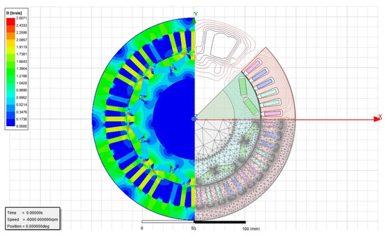
Figure 6.
Electromagnetic model in Ansys Electronics 2022 R2.
Evaluation of Electromagnetic Performances for a Complete Driving Cycle
As mentioned earlier, the WLTP 3 driving cycle is the basis for our optimization process. However, optimizing the motor model using the finite element method can be time-consuming due to the numerous operating points in the driving cycle. To address this challenge, a hybrid approach was devised to mitigate the extensive computational effort required.
To evaluate the efficiency of the motor based on the driving cycle, we need to analyze its performance over a wide working range that covers the operating points of the driving cycle, which allows us to create an efficiency map. The results obtained by varying the phase and amplitude of the current for each speed level are evaluated and compared to select the combination providing the necessary torque at the specific speed with the lowest possible current while respecting the current and amplitude of the converter.
The process of determining the ideal phase and amplitude of the current involves first calculating the line voltage variation with the phase angle of the current. This is then compared to the converter’s voltage limit of 300 V (for example) as illustrated in Figure 7. Upon observation, it is apparent that a phase angle greater than or equal to keeps the line voltage within the limit. Additionally, the maximum torque value is achieved when the phase angle is precisely , as shown in the subsequent figure.
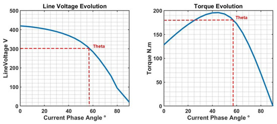
Figure 7.
Determination of the optimal current phase value by analyzing line voltage and torque evolution compared to current phase variation.
To discover the ideal combination of current phase and amplitude, using the finite element (FE) method entails a time-consuming process of repeating the procedure for different current amplitudes across the entire speed range. This results in a lengthy calculation time. To address this, a hybrid method based on finite element simulations dubbed flux mapping was created. Instead of covering the whole operational range, the new method entails scanning the current’s phase and amplitude at a single speed.
The results of the scan will be used to create a mapping of the flow surface. In our case, we will calculate the performance for five current phases and four current amplitude points to generate a flow surface response, as shown in Figure 8.
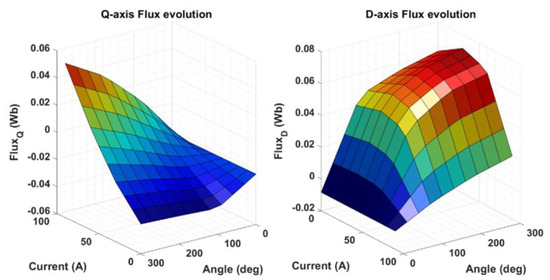
Figure 8.
Direct and quadrature flux cartography according to current phase and amplitude.
In addition, we can use this map to analytically determine the best combination of currents Id, Iq described by the list of the following equations in order to maximize the torque at each speed point in the MTPA (maximum torque per ampere) or FW (field weakening) region while respecting the current and voltage limits, Imax and Umax, of the converter.
- : electromagnetic torque developed;
- p: number of poles;
- : direct and quadrature axis flux;
- : stator phase voltage and current;
- : direct and quadrature axis voltage;
- : direct and quadrature axis current;
- : current angle.
Once the best current values of Id and Iq for the whole operational range of the motor have been found as illustrated in the Figure 9, the next step is to extrapolate losses using the mapping built from the scan findings at a calculated speed. Copper losses, unlike core losses, are only controlled by current amplitude, as indicated in a specific equation, and do not fluctuate with speed. As a result, using the Equation (5), the core losses will be extrapolated to the complete range of speed and torque variation.
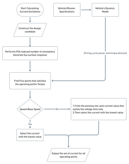
Figure 9.
Current amplitude and phase determination using the simplified method.
- : loss coefficient
- : core losses at reference speed ().
- : reference speed.
The final step involves plotting the efficiency map of the motor after extrapolating the losses on all operating points from the reference speed where the map was created. Table 4 provides a summary of the performance of both comprehensive and hybrid calculation methods in terms of accuracy and calculation time. The maximum error between the two methods is only 4 percent (0.04) which mainly occurs at low speeds, and the efficiency error is well below 1 percent for most of the operating range (Figure 10).
Table 4.
Comparisonof FEA and SemiFEA method results.
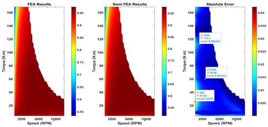
Figure 10.
Comparisons of iso-torque maps calculated by finite element method and hybrid method.
Thermal Model
As mentioned earlier, assessing the temperature of different components is crucial to accurately predict the overall performance and lifespan of the machine, as temperature has a direct impact on these factors. To achieve this, the thermal network method (TNM) is used, which involves dividing the motor into basic thermal components that represent a combination of heat transfer processes involving conduction, convection, and radiation.
The same geometric parameters used in constructing the electromagnetic model will also be utilized for creating the thermal model. This can be seen in Figure 11. The goal is to estimate the temperature of different components of the motor under operating conditions that mimic the Worldwide Harmonized Light Vehicles Test Procedure (WLTP). For this purpose, the Motor-Cad software was employed to create the motor’s thermal circuit (Figure 12), which was then used to perform thermal modeling of the inner permanent magnet motor. Presented in Figure 13 is the temperature distribution across the motor’s thermal circuit for the same operating point used in the finite element model. Thus, the electromagnetic and thermal models are interconnected in such a way that the EF/analytical model of the motor created using Matlab and Ansys Electronics will compute the motor’s performance and electrical losses at the representative operating points of the drive cycle.
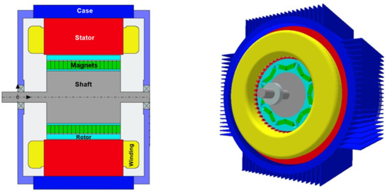
Figure 11.
Motor thermal model on Ansys Motor-Cad V15.
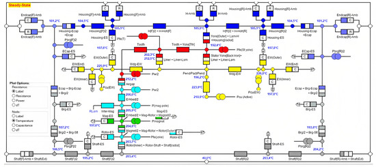
Figure 12.
Motor thermal network on Ansys Motor-Cad V15.
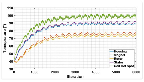
Figure 13.
Temperature evolution in the different components of the motor.
The process of revising the losses and temperature will be repeated until the temperature of the motor is precisely determined, as illustrated in Figure 14 ensuring that the iterative process has converged. Integrating the electromagnetic and thermal models leads to a more in-depth understanding of the motor’s temperature and performance, which in turn facilitates the design and optimization of the motor for real-world applications.
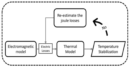
Figure 14.
Motor electro-thermal model connection.
To analyze the temperature of different components of the motor during the WLTP driving cycle, a test was conducted and followed by a resting period to observe the convergence of temperatures. The hybrid electromagnetic model was used to calculate the electrical losses for the entire driving cycle, as shown in Figure 15, along with the rotational speed of the motor shaft. This information will help in understanding the temperature behavior of the motor and optimizing its design for real-world applications.
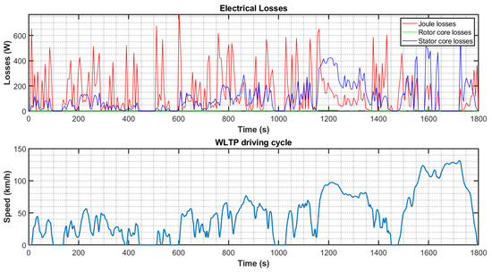
Figure 15.
Electrical losses for the WLTP driving cycle.
The equivalent electrical circuit modeling method provides a way to track the temperature changes in various parts of the motor and has a significantly faster calculation time compared to the time estimated using the finite element modeling method.
Aging Model
The motor’s temperature during the WLTP driving cycle was analyzed through a test followed by a rest period to observe temperature convergence. The hybrid electromagnetic model calculated the electrical losses for the entire driving cycle, as shown in Figure 15, along with the motor shaft’s rotational speed.
Motor aging models are semi-empirical, being based on experimental results under different conditions to establish a mathematical relationship between aging and temperature/time. The motor’s life is closely related to the insulation of its winding, which can cause the motor to malfunction. Therefore, studying the impact of heat on the motor’s lifespan is equivalent to studying the failure of its insulation. The motor’s lifespan can be estimated based on the average temperature during its operation, projected onto a regression curve created from experimental data of motors with the same insulation class, as shown in Figure 16.
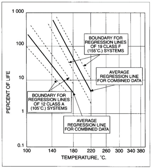
Figure 16.
Evolution of lifetime according to exposition temperature.
Estimating the life of a motor based on average temperature assumes that damage due to temperature is independent of time and is additive, and it does not account for the dynamic evolution of temperature. This type of estimation can yield results close to experimental data, but accuracy is not guaranteed. The residual life factor is defined as the percentage of remaining life between two time references and .
- : represents the lifespan of the motor, which depends on the highest temperature it reaches during operation.
- : the assumed reference lifespan of the motor, which is usually taken to be 20,000 h.
- HIC: refers to the index that measures how much a specific temperature value added to the reference temperature can decrease the lifespan of the motor’s insulation by half.
- TI: denotes the reference temperature that corresponds to the insulation class of the motor.
If the time interval of the excess temperature (,) is extended to period T, the lifetime can be calculated using the following equation.
Motor temperature limits depend on their insulation class, where higher insulation classes allow for higher permissible temperatures at a higher cost. The classification of motor insulation is defined in the scientific literature, and the nomenclature is presented in Table 5.
Table 5.
Insulation classes and maximum temperature ratings.
The relationship mentioned earlier allows for lifetime calculation based not only on simple exponential temperature functions but also on arbitrarily varying motor temperatures over a period T. This can be achieved by digitally integrating variable temperature values based on actual temperature data or simulation results.
Current standard lifetimes expressed in time describe stable and invariable use, while Lp service life includes all periods during which the car is not used. Lp depends on insulation parameters, drive-specific components, thermal losses, behavior, and actual usage function. The interconnection and data exchange between the three sub-models of the farm are summarized in the flowchart in Figure 17.
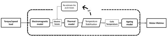
Figure 17.
Multiphysical motor model connection.
2.4. Battery Modeling
2.4.1. Battery Sizing Algorithm
A study was conducted to create an algorithm for sizing a storage system that is capable of meeting the limitations imposed by the battery’s properties and the driving cycle. To size a storage system, the following steps must be taken.
The first step is to estimate the power and energy requirements of the electric vehicle’s mission using the dynamic model of the vehicle. However, this initial evaluation does not take into account the weight of the storage system. Therefore, the total weight (M) is made up of only the weight of the vehicle with a battery weight of zero . Further information on how to size a storage system will be discussed in subsequent sections.
Initial Battery Sizing
The primary step of the sizing algorithm is to calculate the number of cells in a series . This can be achieved by utilizing equations that are based on the voltage value the cell and the bus , which is chosen according to the specific requirements.
The calculation for the number of cells in parallel will be determined by utilizing an equation that factors in the specific energy , weight , and internal resistance of the selected battery technology. To account for the battery’s weight during sizing, a 40% increase is applied to the battery weight, as described in [25].
Updating Vehicle Weight and Estimating Battery Energy
By computing the series and parallel connections of the cells, it becomes feasible to revise the weight of the vehicle without accounting for the storage system’s weight.
The process of sizing the battery also involves determining the amount of energy it can provide, which is calculated based on the depth of discharge (DOD) and the initial capacity of the battery. The equation for calculating the battery capacity is as follows.
:
After updating the weight of the vehicle, the energy and power required for the cycle need to be recalculated to take into account the weight of the storage system. This can be achieved using the following equation:
- : angle of inclination of the road
Sizing of the Battery Taking into Account Its Weight
The final step of the battery sizing process involves repeating the calculation while taking into account the weight of the storage system and its impact on the power and energy demands. This iterative process continues until certain conditions are met, such as the battery capacity being greater than or equal to the energy required for the driving cycle, or the battery weight being less than or equal to the maximum weight allowed for the vehicle. By following these steps, an appropriately sized battery can be selected that meets the requirements of the driving cycle and the limitations of the battery technology.
2.4.2. Multiphysics Battery Modeling
In order to achieve realistic behavior of the battery, the electrical and thermal characteristics of the lithium-ion battery were experimentally observed during a current cycling process. The voltage and internal temperature of the battery were carefully monitored and recorded. These experimental results played a vital role in the development of a multiphysics model that accurately captures the battery’s behavior. By analyzing internal parameters, such as temperature and state of charge (SOC), during both usage and storage, it becomes possible to anticipate the health of the battery. To further enhance the understanding of the battery’s performance during a driving cycle, two sub-models were created to analyze the variations in temperature and SOC. This multiphysics model illustrated in Figure 18 not only enables the early detection of battery degradation but also aids in optimizing battery management strategies.
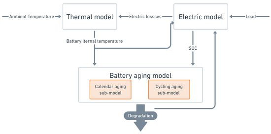
Figure 18.
Battery multiphysical model.
- An electrical model is used to study the electrical phenomena that occur during the driving cycle.
- A thermal model is used to estimate the battery’s temperature by considering the external conditions (ambient temperature) and the changes in internal parameters caused by the electrical phenomena (charge/discharge).
By utilizing the two sub-models, the degradation of battery health can be estimated by continually assessing the electrical parameters of the battery during the driving cycle. The exchange of data and interaction between the sub-models can be observed in the battery multiphysical model diagram. There are different electrical, thermal, and aging models with varying levels of complexity, from the most general to the most specific, due to the various accumulator, format, energy, and composition technologies available. A model tailored to a specific application is often required. In this case, a multiphysics model is used to simulate high-energy NMC electrochemical cells.
Nicolas Damay’s research focuses on an accumulator that is similar to the one used in our case study, where he employs the finite element method for advanced thermal analysis [26]. Other research articles have also utilized this method, such as [27]. However, there are other approaches to thermal modeling of accumulators, including the use of partial differential equations [28], linear systems with varying parameters [29], or equivalent electrical circuits [30].
Due to limitations in conducting extensive tests and the need for fast computations to replicate battery behavior over its lifetime, complex models are challenging to set up and parameterize in our use case using optimization for the identificaiton (Figure 19). Therefore, we opt for an electrical circuit model that is better suited to our needs. The battery type parameters were determined by optimization and minimizing errors in comparison to previously collected experimental data.
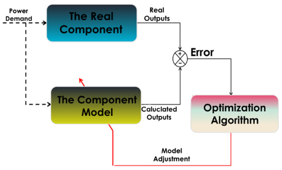
Figure 19.
Identification of model parameters using optimization.
2.5. Optimization Algorithm
It is important to note that the selection of an optimization algorithm depends on the specific problem and its characteristics. While gradient-based optimization algorithms can be more efficient for smooth objective functions, non-gradient-based optimization algorithms such as genetic algorithms can handle non-smooth and non-convex objective functions with multiple optima. Moreover, genetic algorithms can explore a larger solution space and avoid becoming stuck in local optima, making them suitable for multiobjective optimization problems. However, genetic algorithms may require more computational resources and longer convergence times than gradient-based optimization algorithms.
In the end, the choice of optimization algorithm should be based on a careful evaluation of the problem’s characteristics and the available computational resources. The configuration of optimization parameters (Table 6) should also be optimized to obtain the best possible results within the given constraints.
Table 6.
Configuration of optimization parameters.
Below is the updated table in which the order of parameters has changed.
In order to conduct optimization of the design space, it is important to have a wide range of variation in the geometric dimensions. However, the finite element (FE) model must be able to handle large variations in these parameters without resulting in unfeasible configurations that would halt the optimization process. This issue can typically be resolved by including specific constraints in the optimization process to prevent unfeasible configurations while still allowing for a broad range of variation in the design variables. Table 7 displays the fixed range of variation for the optimization parameters.
Table 7.
Optimization parameters—range of variation.
Note: It is critical to ensure that the shaped motor meets all of the operating points of the tested driving cycle, including speed, torque, and power requirements, when optimizing the motor shape. This is critical to ensuring a positive user experience and overall usability of the electric car. If the recommended shape, as determined by the optimization algorithm, does not meet these criteria, it will be rejected and penalized in order to avoid such occurrences in future optimization cycles. By closely adhering to this approach, the optimization process may be centered on discovering motor designs that actually fulfill the performance expectations of the driving cycle, assuring optimal efficiency and user satisfaction.
The objective function takes into account the lifetime of both the motor and the battery. However, since the the motor has a significantly longer service life than that the battery, it is necessary to use a weighting factor to ensure that the optimization does not prioritize the life of the motor over that of the battery or the price of the battery over that of the electric machine.
The weighting factor was determined through several optimization tests to converge toward a balanced solution. Therefore, the objective function combines the minimization of price with the maximization of lifetime, and it can be expressed as follows:
- MSRP: manufacturer’s suggested retail price. This refers to the suggested selling price of the electric vehicle as determined by the manufacturer.
- Prixbatt: battery price.
- Lifetimebatt: lifetime of the battery.
- Prixmoteur: motor price.
- Lifetimemot: lifetime of the electric motor.
3. Results and Discussion
To validate the adopted optimization method and compare the results for different specifications, the optimization process was carried out for the WLTP driving cycle with two different bus voltage settings. The first setting was at 468 V, while the second setting was at 600 V.
The outcomes of the dual optimizations are depicted in the accompanying figure, showcasing the blue population’s convergence toward the red Pareto front, which represents the optimal generation. The inflection point of the Pareto front indicates the elbow, highlighting the most compelling outcomes that strike the optimal balance between the price and lifetime components of the objective function. These outcomes represent the peak of achievable performance and serve as the primary findings of the study.
Firstly, it would be interesting to examine the impact of the bus voltage selection on the battery sizing process. This decision directly influences the weight of the battery, which in turn has a significant effect on the optimization of the motor geometry.
The analysis of the battery mass evolution, as seen in Figure 20, demonstrates the influence of the DC bus voltage on the sizing process. In general, the volume and cost of the storage system exhibit similar trends. Therefore, we rely on the following figure to analyze the results. From this figure, we observe that there are voltage values that lead to optimal sizing, where the storage systeme mass is minimal. The common denominator among these values is the total number (cells in parallel * cell in series) of battery elements, which represents the minimum number of elements capable of providing the energy consumed by the EV.
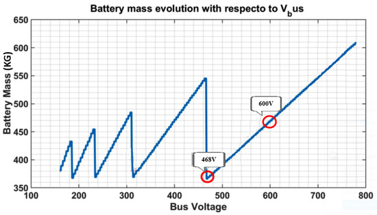
Figure 20.
Battery weight evolution with bus voltage variation.
In the Figure 21 and Figure 22, the values of “Global Lifetime (p.u)” and “Global Price (p.u)” are calculated using a per unit (p.u.) notation. This notation is employed to normalize the values and facilitate the analysis of the curves’ evolution.
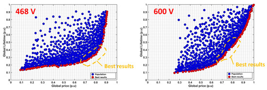
Figure 21.
Optimization results.
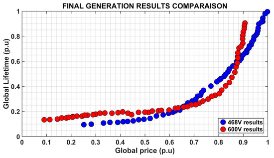
Figure 22.
Final generation optimization results.
To calculate the values of “Global Lifetime (p.u)” and “Global Price (p.u)” in the results, the maximum values of the lifetime and overall cost curves are used as reference points. These maximum values serve as the baseline or 1.0 p.u (100%) reference.
The formulas used to calculate the per unit values are as follows:
Here, “Lifetime” represents the lifetime value at a specific point on the curve, “Maximum Lifetime” is the maximum value obtained from the lifetime curve, “Price” denotes the price value at a specific point on the curve, and “Maximum Price” represents the maximum value obtained from the overall cost curve.
By normalizing the lifetime and price values with respect to their respective maximum values, the curves’ evolution can be represented and compared on a relative scale as in Figure 22. This per unit representation allows for a clearer understanding of the trends and relationships between different scenarios or configurations.
We present an optimization study aimed at finding the optimal geometric design of an electric motor and battery capacity for a given voltage level of the bus in a hybrid electric vehicle. Our objective is to minimize the global cost of the powertrain while maximizing its lifetime.
We performed the optimization for two voltage levels of the bus, 468 V and 600 V, and obtained two populations of optimal solutions that trade-off cost and lifetime. A first glance at the results shows that both optimizations have converged toward a set of optimal solutions represented by the red dots in the Pareto front.
We focused our analysis on the region of the Pareto front located at the elbows, where we can find solutions that are more balanced in terms of cost and lifetime. Among these solutions, we found that the optimization performed for a bus voltage of 468 V showed more promising results in terms of global cost and lifetime.
Our results suggest that a bus voltage of 468 V could be a good compromise between the competing objectives of cost and lifetime. Further studies could investigate the impact of other factors, such as the driving cycle or the weight of the vehicle, on the optimal design of the powertrain.
When comparing the optimization results for the 468 V and 600 V bus voltage levels, we can see that the results cross twice, but the 468 V optimization results are generally more balanced between construction cost and lifetime. The reasons for this can be summarized as follows:
- Lower voltage levels generally lead to higher battery lifetime due to reduced stress on the battery cells. This is because higher voltage levels increase the heat and current density in the battery, which can lead to faster aging and lower lifetime.
- A more optimal voltage level can also reduce the size and cost of the battery pack. This is because a lower voltage level would require fewer cells to achieve requireds power output, which can result in a smaller and less expensive battery pack.
On the other hand, the reasons for the 600 V optimization being better are:
- Higher voltage levels generally lead to higher power output from the electric motor. This is because higher voltage levels allow for higher motor currents, which can result in higher torque and power output.
- A more optimal voltage level can also result in a more efficient electric motor. This is because higher voltage levels can reduce the electrical resistance in the motor windings, which can result in less energy losses and higher efficiency.
- Higher voltage levels can also allow for the use of thinner motor wires, which can reduce the size and weight of the electric motor. This can result in a more compact and lightweight motor design.
- Higher voltage levels also reduce the stress on the electric motor, which can lead to longer motor lifetime. This is because higher voltage levels can result in a lower motor currents and temperatures, which can cause less wear and tear on the motor components over time.
Overall, the choice between the 468 V and 600 V bus voltage levels depends on the specific trade-offs between battery lifetime, motor lifetime, power output, and construction cost. A more optimal voltage level will depend on the specific requirements of the electric vehicle application, such as the desired range, power output, and cost constraints.
The results of the two optimizations show that the choice of bus voltage level has a significant impact on both the battery and the electric motor. However, when considering the trade-off between cost and battery life, the 468 V bus voltage level offers a better balance. For example, if we consider a point with the same battery life (0.4 p.u), we can see that the 600 V level offers more expensive results, mainly due to the over-dimensioning of the battery and the resulting need for a larger motor for vehicle traction. While a higher voltage level means a lower current and therefore smaller magnets, the battery cost outweighs this advantage.
- Bus Voltage Choice Impact on Motor Geometry
We are interested in determining the final geometry of the motor resulting from the realized optimization for the two bus voltage levels as illustrated in Figure 23 and detailed in Table 8. In addition to that are the resulting weights and prices of the motor’s magnets according to the Neodymium’s price in Jan 2022 [31] and a volumic mass of 7650 KG/m represented in Figure 24.
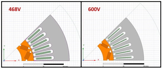
Figure 23.
Motor geometry.
Table 8.
Optimal parameters for the two motors.
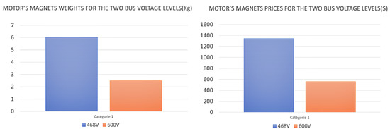
Figure 24.
Motor’s magnet prices and weights.
In this comparison, we analyzed two different motor geometries that operate at different voltage levels. The aim was to identify how changes in the bus voltage from 468 V to 600 V can affect the design parameters of the motors. To accomplish this, we compared the interior diameter of the rotor, exterior diameter of the stator, permanent magnet width and thickness, slot opening, motor length, and coil turns of two motors operating at different voltages. This comparison can help us understand the design considerations that engineers must take into account when designing motors that operate at higher voltage levels.
Interior diameter rotor: With an increase in bus voltage from 468 V to 600 V, the speed of the motor can increase. To maintain the same output power, it may be necessary to reduce the interior diameter of the rotor to increase the torque. This can lead to an increase in the current density in the rotor windings and the generation of more heat. In the case of motor 2, the interior diameter of the rotor is smaller than for motor 1, indicating that a higher torque is required to maintain the same power output due to the higher bus voltage.
Exterior diameter stator: An increase in bus voltage from 468 V to 600 V can also increase the speed of the motor. To maintain high energy efficiency, it may be necessary to increase the exterior diameter of the stator to add more coils and increase the torque. This can lead to an increase in the size and weight of the motor. Motor 2 has a larger exterior diameter of the stator compared to motor 1, indicating that it has more coils and can produce higher torque at a higher bus voltage.
Permanent magnet width and thickness: An increase in bus voltage from 468 V to 600 V can affect the dimensions of the permanent magnets. To maintain the same output power, it may be necessary to reduce the width and thickness of the permanent magnets to maintain the torque. This can affect the magnetic flux density and the holding force of the permanent magnets. In the case of motor 2, the permanent magnet width and thickness are smaller than motor 1, indicating that the permanent magnets are designed to operate efficiently at a higher bus voltage.
Slot opening: An increase in bus voltage from 468 V to 600 V can affect the width of the slots between the teeth of the stator. To maintain high energy efficiency, it may be necessary to reduce the width of the slots to increase the coil density and torque. This can affect the noise, friction losses, and wear of the stator. In the case of motor 2, the slot opening is smaller than motor 1, indicating that the coil density is higher and can produce more torque at a higher bus voltage.
Motor length: An increase in bus voltage from 468 V to 600 V can affect the length of the motor. To maintain high energy efficiency, it may be necessary to reduce the length of the motor to reduce the resistance of the windings and the losses due to Foucault currents. This can affect the current density, heat generation, and thermal dissipation. In the case of motor 2, the motor length is smaller than motor 1, indicating that it is designed to operate efficiently at a higher bus voltage.
Coil turns: With an increase in bus voltage from 468 V to 600 V, the number of coil turns may also need to be increased to maintain the same output power and torque. This can affect the coil density, current density, and heat generation. In the table, motor 2 has more coil turns than motor 1, indicating that it is designed to operate efficiently at a higher bus voltage. However, it is important to note that the specific number of coil turns for each motor is not provided in the table, so a direct comparison cannot be made.
3.1. Bus Impact of Voltage Choice on Battery Sizing and Price
When considering the choice of voltage level for an electric vehicle, various factors come into play. Let us discuss the technical aspects and examine why one voltage level may be preferable over the other while also considering the implications of price and weight as showen in the Figure 25.
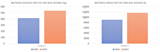
Figure 25.
Battery prices and weights.
Performance: A higher voltage level, such as 600 V, can deliver more power to the electric motors, resulting in improved overall performance in terms of acceleration and top speed. Electric motors tend to operate more efficiently at higher voltages and can be designed for higher power outputs. However, it is important to note that increased voltage does not automatically guarantee better performance, as other factors such as component capacity and overall system optimization must also be considered.
Price: Battery costs are typically influenced by the number of cells used. Achieving a higher voltage level, such as 600 V, requires more cells, resulting in increased battery costs. Conversely, a 468 V battery requires fewer cells, leading to reduced overall battery costs. Therefore, opting for a 468 V battery can offer significant financial savings compared to a 600 V battery.
Weight: Battery weight is also closely tied to the number of cells utilized. Higher voltages necessitate more cells, resulting in a heavier battery. The additional weight of the cells can impact vehicle maneuverability, energy efficiency, and range. Consequently, a 468 V battery can help reduce the overall weight of the electric vehicle, providing benefits in terms of improved range, performance, and efficiency.
Safety: Safety is a crucial aspect in electrical system design, especially in electric vehicles. Higher voltages, such as 600 V, increase the risk of electrical shock and safety issues. Enhanced safety measures, such as reinforced insulation, are necessary to ensure safe operation at higher voltages. This can add complexity to the design and incur additional costs to meet the required safety standards. On the other hand, a 468 V battery voltage poses fewer potential safety risks. Electrical components can be designed for lower voltage levels, reducing the risk of electrical shock and facilitating the implementation of appropriate safety measures. This simplifies the system design, reduces costs associated with additional safety measures, and ensures safer operation of the electric vehicle.
Volume: The size and volume of the battery can significantly impact the available space inside the vehicle. Higher voltages, such as 600 V, require more cells, resulting in increased overall battery volume. This may reduce interior space, compromise cargo capacity, or restrict interior layout options. In contrast, a 468 V battery requires fewer cells, resulting in a reduced battery volume. This frees up interior space for passengers, luggage storage, or other equipment. Additionally, a smaller battery volume facilitates better integration into the overall vehicle design, offering more flexibility for designers.
In conclusion, a 468 V battery offers advantages in terms of cost, weight, safety, and volume compared to a 600 V battery. While higher voltage may provide performance benefits, it is crucial to evaluate the trade-offs between performance, cost, weight, safety, and available interior space when selecting the appropriate battery voltage for a specific electric vehicle.
3.2. Further Cost Implications of Bus Voltage Selection
3.2.1. Power Electronics and Control Systems
The choice of bus voltage in an electric vehicle has a significant impact on the cost of power electronics and control systems. When opting for higher bus voltages, more advanced and complex components such as inverters and converters are required to handle the increased voltage levels. These components often involve sophisticated semiconductor technologies, resulting in higher manufacturing and material costs. Additionally, high-voltage systems may necessitate additional safety features and specialized components, further contributing to the overall cost. Conversely, lower bus voltage systems may offer cost advantages with simpler and more readily available power electronics and control systems. It is crucial to carefully consider the cost implications of different bus voltage levels to ensure an optimal balance between performance and cost-effectiveness.
3.2.2. Wiring and Distribution
The choice of bus voltage also impacts the wiring and distribution infrastructure within the electric vehicle. Higher voltage systems generally allow for the use of smaller-gauge wires and cables due to reduced current levels, resulting in cost savings. However, high-voltage systems may require additional insulation and safety measures to ensure proper electrical isolation and protection, potentially increasing material and manufacturing costs. Moreover, specialized connectors and interfaces may be necessary for high-voltage systems, adding to the overall cost. Conversely, lower voltage systems may require thicker wires to handle higher currents, which can contribute to increased material costs. Careful evaluation of the bus voltage’s impact on wiring and distribution is essential to optimize cost without compromising safety and performance.
3.2.3. Charging Infrastructure
The selection of bus voltage in an electric vehicle has a significant impact on the required charging infrastructure. Higher voltage systems, such as those operating at 800 V, are typically associated with fast-charging solutions. These systems demand specialized charging stations and equipment capable of handling the increased power levels. The charging infrastructure needs to be designed to accommodate the higher voltages, requiring robust electrical components, advanced cooling systems, and enhanced safety features. Consequently, the installation and operation of high-voltage charging infrastructure tend to be more complex and costly.
In contrast, lower voltage systems, such as those operating at 400 V, can leverage existing charging infrastructure, such as standard AC charging stations. These lower voltage systems offer a more cost-effective solution, as they do not require extensive modifications or specialized equipment. However, it is important to note that charging speeds may be slower with lower voltage systems compared to their high-voltage counterparts.
3.2.4. Cost and Size of the Gearbox
Higher bus voltages in electric vehicles lead to reduced current levels flowing through the motor. Consequently, the torque and power demands on the motor decrease. This reduction in torque and power requirements allows for the design of smaller gearboxes with lower gear ratios. Smaller gearboxes typically have fewer components and employ lighter materials, resulting in cost savings during manufacturing and material procurement.
On the other hand, lower bus voltages require higher current levels to achieve the desired torque and power outputs. The increased current demand necessitates larger and more robust motors, which in turn require larger gearboxes to handle the higher forces involved. Larger gearboxes often feature more complex designs, additional components, and stronger materials, leading to increased manufacturing and material costs.
3.2.5. Component Integration
The chosen bus voltage level influences the integration of various components within the powertrain system. Different voltage levels may require specific connectors, interfaces, and compatibility considerations, which can influence component costs. Higher voltage systems may necessitate specialized connectors and interfaces capable of handling the increased electrical potential, leading to higher component costs. Conversely, lower voltage systems may utilize more standardized components, resulting in potential cost savings. The choice of bus voltage should carefully consider the impact on component integration costs, ensuring compatibility, reliability, and cost-effectiveness throughout the powertrain system.
By thoroughly analyzing the cost implications associated with varying bus voltage levels, decision-makers can assess the financial impact on the powertrain system. Considering the costs of power electronics, control systems, wiring and distribution, charging infrastructure, and component integration allows for the development of cost-effective and efficient electric vehicle powertrains. Striking a balance between performance, efficiency, and overall cost is crucial for achieving widespread adoption and market competitiveness.
4. Conclusions
Our goal was to optimize the lifetime and overall cost of the powertrain, taking into account the various multiphysics aspects of the motor as well as the battery sizing and optimization, to create a more holistic approach to powertrain optimization.
To estimate the lifetime of the motor and battery, we developed several analytical and finite element hybrid models that account for various electrical, thermal, and aging factors. These models allowed us to identify the optimal population of motor shapes that provide the best balance between cost and powertrain lifetime.
After comparing the optimization results, we found that both the 468 V and 600 V levels converged toward an optimal population that presented the best balance between powertrain lifetime and construction cost. However, depending on the region of interest, the results could be better for one voltage level than the other. For example, if reducing battery size and cost is the primary concern, a lower voltage level may be more suitable. Conversely, if optimizing motor lifetime and reducing cost are the main concerns, a higher voltage level may be more appropriate.
In addition to analyzing the impact of the voltage levels on the motor geometry, it is also important to consider the impact on other powertrain components and overall system design when choosing the optimal voltage level. For example, a higher voltage level may allow for more efficient power transfer and reduce losses in other powertrain components. However, it may also require more advanced electronics and control systems, which could increase the system’s complexity and cost. On the other hand, a lower voltage level may simplify the system and reduce costs but may also result in reduced efficiency and performance. Therefore, a comprehensive analysis of all factors must be considered when selecting the optimal voltage level for the powertrain.
In conclusion, our study highlights the importance of taking a holistic approach to powertrain optimization that considers all the relevant multiphysics aspects. We believe that our findings can help guide future research and development efforts aimed at improving the performance and reducing the cost of electric vehicle powertrains.
Author Contributions
Conceptualization, A.R.M. and N.R.; methodology, A.R.M. and N.R.; software, A.R.M.; validation, A.R.M., N.R. and P.L.; formal analysis, A.R.M.; investigation, A.R.M.; resources, A.R.M., C.V., R.B. and C.L.; data curation, A.R.M., C.V., R.B. and C.L.; writing—original draft preparation, A.R.M.; writing—review and editing, A.R.M., N.R., P.L., C.V., R.B. and C.L.; visualization, A.R.M.; supervision, A.R.M.; project administration, A.R.M. All authors have read and agreed to the published version of the manuscript.
Funding
This research received no external funding.
Data Availability Statement
Not applicable.
Conflicts of Interest
The authors declare no conflict of interest.
References
- Sanguesa, J.A.; Torres-Sanz, V.; Garrido, P.; Martinez, F.J.; Marquez-Barja, J.M. A Review on Electric Vehicles: Technologies and Challenges. Smart Cities 2021, 4, 372–404. [Google Scholar] [CrossRef]
- Chan, C.C. The State of the Art of Electric, Hybrid, and Fuel Cell Vehicles. Proc. IEEE 2007, 95, 704–718. [Google Scholar] [CrossRef]
- Yang, Y.P.; Shih, G.Y. Optimal Design of an Axial-Flux Permanent-Magnet Motor for an Electric Vehicle Based on Driving Scenarios. Energies 2016, 9, 285. [Google Scholar] [CrossRef]
- Albatayneh, A.; Assaf, M.N.; Alterman, D.; Jaradat, M. Comparison of the Overall Energy Efficiency for Internal Combustion Engine Vehicles and Electric Vehicles. Environ. Clim. Technol. 2020, 24, 669–680. [Google Scholar] [CrossRef]
- Agamloh, E.; von Jouanne, A.; Yokochi, A. An Overview of Electric Machine Trends in Modern Electric Vehicles. Machines 2020, 8, 20. [Google Scholar] [CrossRef]
- Yong, J.Y.; Ramachandaramurthy, V.K.; Tan, K.M.; Mithulananthan, N. A review on the state-of-the-art technologies of electric vehicle, its impacts and prospects. Renew. Sustain. Energy Rev. 2015, 49, 365–385. [Google Scholar] [CrossRef]
- Sieklucki, G. Optimization of Powertrain in EV. Energies 2021, 14, 725. [Google Scholar] [CrossRef]
- Cai, W.; Wu, X.; Zhou, M.; Liang, Y.; Wang, Y. Review and Development of Electric Motor Systems and Electric Powertrains for New Energy Vehicles. Automot. Innov. 2021, 4, 3–22. [Google Scholar] [CrossRef]
- El Hadraoui, H.; Zegrari, M.; Chebak, A.; Laayati, O.; Guennouni, N. A Multi-Criteria Analysis and Trends of Electric Motors for Electric Vehicles. World Electr. Veh. J. 2022, 13, 65. [Google Scholar] [CrossRef]
- Mazali, I.I.; Daud, Z.H.C.; Hamid, M.K.A.; Tan, V.; Samin, P.M.; Jubair, A.; Ibrahim, K.A.; Kob, M.S.C.; Xinrui, W.; Talib, M.H.A. Review of the Methods to Optimize Power Flow in Electric Vehicle Powertrains for Efficiency and Driving Performance. Appl. Sci. 2022, 12, 1735. [Google Scholar] [CrossRef]
- Koch, A.; Teichert, O.; Kalt, S.; Ongel, A.; Lienkamp, M. Powertrain Optimization for Electric Buses under Optimal Energy-Efficient Driving. Energies 2020, 13, 6451. [Google Scholar] [CrossRef]
- Ansys Maxwell 2022 R2 | Logiciel d’analyse de dispositifs électromécaniques. Available online: https://www.ansys.com/fr-fr/products/electronics/ansys-maxwell (accessed on 12 April 2023).
- Ansys Electronics 2022 R2 | Electronic Design and Electromagnetics Simulation. Available online: https://www.ansys.com/products/electronics (accessed on 3 February 2023).
- Rimpas, D.; Kaminaris, S.D.; Piromalis, D.D.; Vokas, G.; Arvanitis, K.G.; Karavas, C.S. Comparative Review of Motor Technologies for Electric Vehicles Powered by a Hybrid Energy Storage System Based on Multi-Criteria Analysis. Energies 2023, 16, 2555. [Google Scholar] [CrossRef]
- Ehsani, M.; Gao, Y.; Gay, S. Characterization of electric motor drives for traction applications. In Proceedings of the IECON’03. 29th Annual Conference of the IEEE Industrial Electronics Society (IEEE Cat. No.03CH37468), Roanoke, VA, USA, 2–6 November 2003; Volume 1, pp. 891–896. [Google Scholar] [CrossRef]
- Jokar, A.; Rajabloo, B.; Désilets, M.; Lacroix, M. An Inverse Method for Estimating the Electrochemical Parameters of Lithium-Ion Batteries: I. Methodology. J. Electrochem. Soc. 2016, 163, A2876. [Google Scholar] [CrossRef]
- Ravindra Jape, S.; Thosar, A. Comparison of Electric Motors for Electric Vehicle Application. Int. J. Res. Eng. Technol. 2017, 6, 12–17. [Google Scholar] [CrossRef]
- Rahman, Z.; Ehsani, M.; Butler, K.L. An Investigation of Electric Motor Drive Characteristics for EV and HEV Propulsion Systems; SAE Technical Paper 2000-01-3062; SAE International: Warrendale, PA, USA, 2000; ISSN 0148-7191/2688-3627. [Google Scholar] [CrossRef]
- Eudy, L.; Zuboy, J. Overview of Advanced Technology Transportation, 2004 Update; National Renewable Energy Laboratory: Golden, CO, USA, 2004; p. 24. [Google Scholar]
- Bluecar Blue Systems. Available online: https://www.bluesystems.fr/technology/bluecar/ (accessed on 16 June 2023).
- Mock, P. World-Harmonized Light-Duty Vehicles Test Procedure; International Council on Clean Transportation: San Francisco, CA, USA, 2013. [Google Scholar]
- Meddour, A.; Rizoug, N.; Babin, A. The influence of driving cycle characteristics on motor optimisation for electric vehicles. In Proceedings of the 2022 30th Mediterranean Conference on Control and Automation (MED), Vouliagmeni, Greece, 28 June–1 July 2022; pp. 43–48, ISSN 2473-3504. [Google Scholar] [CrossRef]
- Norme WLTP: Définition, Impact et Différences ENGIE Mobilité Verte. Available online: https://mobiliteverte.engie.fr/conseils-et-actualites/vehicule-electrique/norme-wltp-definition-impact-differences.html (accessed on 16 June 2023).
- Power to Move the World (No Date) XALT Energy. Available online: https://www.xaltenergy.com/ (accessed on 16 June 2023).
- Sadoun, R.; Rizoug, N.; Bartholomeüs, P.; Barbedette, B.; Le Moigne, P. Optimal sizing of hybrid supply for electric vehicle using Li-ion battery and supercapacitor. In Proceedings of the 2011 IEEE Vehicle Power and Propulsion Conference, Chicago, IL, USA, 6–9 September 2011; pp. 1–8, ISSN 1938-8756. [Google Scholar] [CrossRef]
- Damay, N.; Forgez, C.; Bichat, M.P.; Friedrich, G.; Ospina, A. Thermal modeling and experimental validation of a large prismatic Li-ion battery. In Proceedings of the IECON 2013—39th Annual Conference of the IEEE Industrial Electronics Society, Vienna, Austria, 10–13 November 2013; pp. 4694–4699. [Google Scholar] [CrossRef]
- Pruteanu, A.; Florean, B.V.; Moraru, G.M.; Ciobanu, R.C. Development of a thermal simulation and testing model for a superior lithium-ion-polymer battery. In Proceedings of the 2012 13th International Conference on Optimization of Electrical and Electronic Equipment (OPTIM), Brasov, Romania, 24–26 May 2012; pp. 947–952, ISSN 1842-0133. [Google Scholar] [CrossRef]
- PDE model for thermal dynamics of a large Li-ion battery pack. In Proceedings of the 2011 American Control Conference, San Francisco, CA, USA, 29 June–1 July 2011.
- Alaoui, C. Solid-State Thermal Management for Lithium-Ion EV Batteries. IEEE Trans. Veh. Technol. 2013, 62, 98–107. [Google Scholar] [CrossRef]
- Forgez, C.; Vinh Do, D.; Friedrich, G.; Morcrette, M.; Delacourt, C. Thermal modeling of a cylindrical LiFePO4/graphite lithium-ion battery. J. Power Sources 2010, 195, 2961–2968. [Google Scholar] [CrossRef]
- Neodymium Price Today—Historical Chart; Forecast—How to Buy (2023) Strategic Metals Invest. Available online: https://strategicmetalsinvest.com/neodymium-prices/ (accessed on 16 June 2023).
Disclaimer/Publisher’s Note: The statements, opinions and data contained in all publications are solely those of the individual author(s) and contributor(s) and not of MDPI and/or the editor(s). MDPI and/or the editor(s) disclaim responsibility for any injury to people or property resulting from any ideas, methods, instructions or products referred to in the content. |
© 2023 by the authors. Licensee MDPI, Basel, Switzerland. This article is an open access article distributed under the terms and conditions of the Creative Commons Attribution (CC BY) license (https://creativecommons.org/licenses/by/4.0/).