Oil Price Forecasting Using FRED Data: A Comparison between Some Alternative Models

Abstract

This paper investigates the forecasting accuracy of alternative time series models when augmented with partial least-squares (PLS) components extracted from economic data, such as Federal Reserve Economic Data, as well as Monthly Database (FRED-MD). Our results indicate that PLS components extracted from FRED-MD data reduce the forecasting error of linear models, such as ARIMA and SARIMA, but produce poor forecasts during high-volatility periods. In contrast, conditional variance models, such as ARCH and GARCH, produce more accurate forecasts regardless of whether or not the PLS components extracted from FRED-MD data are used.

1. Introduction

Energy consumption is required to power the worldwide economy, including most human activities [1]. Accordingly, nearly all worldwide industrial production activities, transportation systems, economic development projects, and machinery and equipment rely upon the energy production and distribution of oil, natural gas, coal, electricity, biofuels, waste, and other sources of supply and their derivatives to enable all of these integrated components of the worldwide economy to function [2]. This also means that energy prices that fuel all parts of the supply chain distribution system are a vital fraction of the price of every commercial product that requires shipping and electrical products to function [3].

Because of this dependence, unexpected steep increases in energy prices can suppress economic growth. They could generate inflation in countries that are net importers of oil, depending upon circumstances, duration, the type of oil, existing inventory, the size of the nation, energy substitution capability, and the number of industries affected [4,5]. Conversely, substantial energy price drops create serious budgetary problems for oil-exporting countries [6]. At present, oil, which is by far the most highly consumed and concentrated energy source, provides somewhere between 30–35% of all of the energy needed to run the global economy, which is 5–10% more than coal, 10–15% more than natural gas, and 25–30% more than renewable and nuclear energy [7].

Despite the importance of energy in human activities, there needs to be more consensus on the roles of energy consumption and energy pricing mechanisms [8]. Historical examples such as oil demand shocks in the price of oil in 1973/74, 1979/80, 1986, 1997/2000, and 2003/2008 are examples of complex events that have both stimulating and depressing effects on national economies. There is also a lack of consensus about the predictive accuracy of energy commodity pricing models, e.g., [9,10]. The lack of understanding of how oil prices are developed and structured has resulted in unexpected, international high and low oil price volatility, spikes, and supply and demand shocks. Price volatility has a significant impact on global financial markets, economic development activity, and political stability, as well as on automobile fuel prices, airline transportation prices, and shipping rates. It also financially impacts national economies and consumer goods and services.

To alleviate the oil price modeling challenges, researchers have used a panoply of models spanning from Stevenson and Bear’s [11] most trivial random walk to highly sophisticated nonlinear models, such as dynamic model averaging, not to mention the recent advances in commodity forecasting using machine learning models. Most of the literature on commodity price forecasting can be grouped into three categories: univariate time series, multivariate time series, and volatility forecasting. In turn, under each category, researchers have used linear and nonlinear models with and without exogenous variables.

The autoregressive and moving average (ARMA) model of Box and Jenkins [12] and its variants are widely used in time series forecasting. ARMA models stipulate that a stationary (A time series is stationary if its mean, variance, and covariance do not vary with time. If the series is not stationary, we can integrate it to make it stationary by taking successive differences, yielding an autoregressive integrated moving average (ARIMA) process) time series can be modeled as a weighted average of its past observations (AR process) and the past observations of the white noise process. The literature abounds with studies that use ARIMA as either a forecasting tool or a benchmark in predicting commodity prices, for example, [13,14,15,16] for oil prices, [17] for electricity prices, and [18] gold.

There are other variations of the ARIMA model, such as the seasonal autoregressive integrated moving average or SARIMA, the controlled autoregressive integrated segmented moving average or CARISMA [19], the fuzzy autoregressive integrated moving average or FARIMA [20], and the fuzzy seasonal autoregressive integrated moving average (FSARIMA) that combines the seasonal SARIMA with the fuzzy regression model [21]. The ARIMA model, Poisson, Markov, autoregressive, moving average, ARMA, and ARIMA processes are limited to short-range dependencies. In addition, the autoregressive fractional integral moving average model (ARFIMA) is identified as a fractional order signal processing technique as a generalization of the ARIMA and the ARMA models [22]. Because of this integration, the authors of [22] found the ARFIMA to offer broader applications than all of the previously mentioned time series analysis methodologies with both short-term and long-term dependence. In addition, the authors found the ARFIMA forecasting model to result in a superior fit compared with established integer-order models when working with spatial or time series data with long-range dependence (LRD), that is, long-memory or long-range persistence.

To overcome the limitations of the ARMA and its variant models, some researchers investigate whether oil price time series portray long-memory properties or volatility (see, for example, [23,24,25,26,27]). However, with evidence of nonlinear dependence, predictable returns, and volatility, long-memory properties contradict the validity of weak-form oil market efficiency. Although, at the same time, some studies have empirically tested the modeling and forecasting of long-memory fluctuations in crude oil markets with the use of generalized autoregressive conditional heteroskedasticity (GARCH) type models (e.g., [28,29,30,31]; researchers conducting these studies still think that long memories and volatility that appear in returns are irrelevant. Nevertheless, because it has been well-known that market shocks have a substantial simultaneous influence on returns and volatility, they have dual long-memory properties. Thus, based on this, researchers such as [32,33,34,35] use the joint ARFIMA-FIGARCH model to study the relationship between returns and volatility in economic and financial time series. This model is well suited to conducting such an analysis of a process demonstrating dual long-memory properties.

The recent availability of economic data, such as the Federal Reserve Economic Data (FRED) (For a detailed description of the FRED data, see [36]) and the Economic Policy Uncertainty data (EPU; the authors of [37] have presented new research perspectives to use the exogenous variable approach to forecast oil prices. For instance, the authors of [38] use FRED and EPU datasets and other financial variables to predict crude oil prices using various machine learning models. However, these data exhibit high multicollinearity among their variables. For instance, Appendix Table A1 indicates that approximately 50% of the variables in FRED data show a correlation coefficient greater than 0.50 in absolute value, with more than 26% exhibiting a correlation coefficient greater than 0.75.

The high correlation coefficient and dimensionality of big data, such as FRED, make data reduction techniques suitable by projecting the high dimension data onto a few orthogonal components, eliminating multicollinearity, and reducing the computational cost when the big set is used (for instance, the dynamic model averaging, introduced by [39], does not allow more than 30 variables in the DMA R package). Principal component analysis (PCA) appears to be a popular choice among researchers in the area of economics and finance (see, for example, [40,41,42,43]). The partial least squares (PLS) method is another data reduction technique to avoid the multicollinearity problem while taking advantage of the data pattern. While the PCA technique uses only the explanatory variables to extract the principal components without considering how each variable relates to the dependent variable, the partial least squares method offers an alternative approach to PCA by capturing the relationship between explanatory variables and dependent variables when extracting the components.

This paper assesses the out-of-sample forecasting accuracy of several time series models in predicting the West Texas Intermediate (WTI) crude oil prices. We consider a basic ARIMA model, a seasonal ARIMA (SARIMA), the partial least squares using FRED economic data, augmented ARIMA and SARIMA models with exogenous variables (the PLS components, COVID-19, and the 2008 financial crisis dummy variables), an autoregressive conditional heteroskedasticity model (ARCH), and a generalized autoregressive conditional heteroskedasticity model (GARCH). We also ask and answer the following question: Can economic data, such as FRED, improve oil forecasting accuracy? We compare these alternative models using the mean absolute (MAE), the mean absolute percentage error (MAPE), and the root-mean-squared error (RMSE) of the out-of-sample predictions.

This paper adds to the existing literature on oil price forecasting in at least two aspects. First, we combine mean and variance models to produce more accurate oil price forecasts. The results show that considering the volatility equation along the mean equation improves the forecasting accuracy by 70%. Second, we use the FRED data after reducing its dimension using partial least-squares. This is crucial as the original FRED data are characterized by a high correlation among most variables, potentially inducing overfitting.

The rest of the paper is organized as follows. First, in Section 2, we describe the alternative models used for prediction. Then, Section 3 describes the data and estimation issues. Finally, in Section 4 and Section 5, we present and discuss the results; in Section 6, we conclude and suggest future research avenues.

2. Methods

We start this section by presenting the partial least squares method to extract the most relevant components from FRED economic data, to explain the variation in crude oil price WTI. Then, we present ARIMA and SARIMA models and their variants and close the section by describing the ARCH-GARCH models.

2.1. Partial Least Squares

The starting point is the research’s goal to explain the variation of the dependent variable y by the variation of the explanatory variables X. However, using the linear regression $y=X\beta +ϵ$ poses the issue of collinearity in the variables of the matrix X. To overcome this issue, in the case of principal component analysis, the matrix X of explanatory variables is decomposed into a smaller set of uncorrelated components. While PCA extracts the features without considering the dependent variable y, the partial least squares extract the components by maximizing the covariance between y and X. We project the explanatory variable space into components z, such as $z=v^{\prime }X$ with $v^{\prime }v=I$, where I is the identity matrix. Similarly, we project the dependent variable space into components r, such that $r=w^{\prime }y$, where $w^{\prime }w=I$ (y canrepresent multivariate dependent variables. In this study, y represents the oil price.) The loading factors v and w are then found by maximizing the covariance between the loading scores z and r, that is,

$$\begin{array}{c}\hfill maxE\left[zr\right]=maxE[v^{\prime }X{w}^{\prime }y]\\ \hfill subjectto{v}^{\prime }v=Iand{w}^{\prime }w=I\end{array}$$

(1)

With v at hand, we can predict the dependent variable as $y=z\gamma =v^{\prime }X\gamma$. Another alternative is to use a set of components explaining a given level of variance in y as regressors instead of X.

2.2. ARIMA-SARIMA Models

In these models, the dependent variable $y_t$ is a weighted average of the past value of $y_t$ and a white noise error term ${ϵ}_t$, that is,

$$y_t=\delta +{\theta }_1{y}_{t-1}+{\theta }_2{y}_{t-2}+\cdots +{\theta }_p{y}_{t-p}+{ϵ}_t+{\alpha }_1{ϵ}_{t-1}+{\alpha }_2{ϵ}_{t-2}+\cdots +{\alpha }_{t-q}{ϵ}_{t-q},$$

(2)

where p is the number of autoregressive processes (AR) and q is the number of moving average processes (MA). The dependent variable needs to be stationary; otherwise, it should be differenced as many times as necessary to make it stationary, yielding the integration order, d. So, an $\mathrm{A}\mathrm{R}\mathrm{I}\mathrm{M}\mathrm{A}(p,d,q)$ is a process that has been differenced d times and decomposed into p AR and q MA processes.

In addition, some time series exhibit seasonality in the $\mathrm{AR}$, the d, and the $\mathrm{MA}$ processes. Therefore, the ARIMA model is modified accordingly, yielding the seasonal ARIMA model or SARIMA. The following equation summarizes the SARIMA model:

$$\begin{array}{c}\hfill y_t=\delta +\sum _{j=1}^p{\theta }_j{y}_{t-j}+\sum _{l=1}^P{\varphi }_l{y}_{t-l\times s}-\sum _{j=1}^p\sum _{l=1}^P{\theta }_j{\varphi }_l{y}_{t-l\times s-j}\\ \hfill +\sum _{m=1}^q{\alpha }_m{ϵ}_{t-m}+\sum _{k=1}^Q{\lambda }_k{ϵ}_{t-k}+\sum _{m=1}^q\sum _{k=1}^Q{\alpha }_m{\lambda }_k{ϵ}_{t-k\times s-m}+{ϵ}_t,\end{array}$$

(3)

where P indicates the number of seasonal autoregressive terms, Q represents the number of moving average terms, and s is the number of seasonal periods (for example, $s=12$ for monthly data, and $s=4$ for quarterly data). For instance, $\mathrm{S}\mathrm{A}\mathrm{R}\mathrm{I}\mathrm{M}\mathrm{A}(p=1, d=0,$${q=1)(P=1, D=0, Q=1)}_{s=12}=\mathrm{S}\mathrm{A}\mathrm{R}\mathrm{I}\mathrm{M}\mathrm{A}(1,0,1){(1,0,1)}_{12}$ is given by:

$$\begin{array}{c}\hfill y_t=\delta +{\theta }_1{y}_{t-1}+{\varphi }_1{y}_{t-12}-{\theta }_1{\varphi }_1{y}_{t-13}\\ \hfill +{\alpha }_1{ϵ}_{t-1}+{\lambda }_1{ϵ}_{t-12}+{\alpha }_1{\lambda }_1{ϵ}_{t-13}+{ϵ}_t\end{array}$$

(4)

In addition, the ARIMA and SARIMA models can be extended to include exogenous variables. This study will add partial least squares components to ARIMA and SARIMA to create ARIMAX and SARIMAX models.

2.3. ARCH-GARCH Models

The ARIMA, ARIMAX, SARIMA, and SARIMAX models assume the variance is constant over time and therefore do not capture the time-varying volatility commodity prices exhibit. One of the stylized facts of financial time series is volatility clustering: periods of high volatility follow periods of high volatility, and vice versa [44]. To account for volatility clustering, the mean equation model is augmented by the variance equation. There are two main approaches to modeling volatility: the autoregressive conditionally heteroscedastic (ARCH) model and the generalized autoregressive conditionally heteroscedastic (GARCH) model. The ARCH model, introduced by [45], simultaneously models the mean of the time series $y_t$ and the shocks variance ${\sigma }_t^2$ as follows:

$$\begin{array}{c}\hfill y_t=\mu +{ϵ}_t\\ \hfill {\sigma }_t^2=\omega +{\alpha }_1{ϵ}_{t-1}^2+{\alpha }_2{ϵ}_{t-2}^2+\cdots +{\alpha }_r{ϵ}_{t-r}^2+{\eta }_t,\end{array}$$

(5)

where ${\eta }_t$ is a white noise process. Here, $\mu$ can follow any process described in the previous section, such as ARIMA or SARIMA. We obtain the GARCH model by adding lagged shock variances as suggested by [46]. Hence, the model in Equation (5) becomes:

$$\begin{array}{c}\hfill y_t=\mu +{ϵ}_t\\ \hfill {\sigma }_t^2=\omega +{\alpha }_1{ϵ}_{t-1}^2+{\alpha }_2{ϵ}_{t-2}^2+\cdots +{\alpha }_r{ϵ}_{t-r}^2+{\beta }_1{\sigma }_{t-1}^2+{\beta }_2{\sigma }_{t-2}^2+\cdots +{\beta }_o{\sigma }_{t-o}^2+{\eta }_t.\end{array}$$

(6)

The use of these panoplies of models allows the researchers to benefit from their advantages and avoid their disadvantages. For example, the linear models of ARIMA and SARIMA present the advantage of linearity and parsimony that are simple to estimate. However, most financial and economic time series are highly nonlinear, implying the failure of linear models to provide better forecasts. To avoid this disadvantage, volatility models (ARCH and GARCH) are necessary, especially if the time series shows periods of volatility clustering, as in the case of crude oil prices. Nevertheless, when there is an asymmetry in the volatility clustering between good news and bad news, the GARCH models are inadequate.

3. Data and Estimation Strategy

3.1. Data

The data used in this study consist of monthly West Texas Intermediate crude oil prices obtained from the U.S. Energy Information Administration (EIA) and the Federal Reserve Economic Data-Monthly Database (FRED-MD) from February 1992 to October 2022. The FRED-MD data consist of 128 economic variables (FRED-MDalso has an oil price variable, but we excluded it and used WTI from US-EIA), classified into eight groups: (1) output and income, (2) labor market, (3) consumption and orders, (4) orders and inventories, (5) money and credit, (6) interest rate and exchange rates, (7) prices, and (8) the stock market. (Giventhe big number of variables in FRED-MD data, we do not provide descriptive statistics for this data. Interested readers are referred to [36] for a thorough description of the FRED-MD data.).

Table 1 provides descriptive statistics of the oil prices and the percentage change in the oil price (price return), defined as $r_t=100\ast \frac{p_t-p_{t-1}}{p_{t-1}}$, during the period of study. The WTI prices averaged $51.27 a barrel and had a standard deviation of $29.50 a barrel, indicating the high volatility of the oil prices during this period. The oil prices oscillated between a minimum of $11.28 a barrel and a maximum of $133.93 a barrel with relatively low skewness (0.53) and kurtosis (−0.81).

Table 1. Summary statistics of oil prices.

	Observations	Mean	Std.Dev.	Min	Max	Skewness	Curtosis
Oil price	368	51.27	29.50	11.28	133.93	0.53	−0.81
Price return	367	0.79	8.51	−42.20	34.14	−0.44	2.33

Figure 1 shows the monthly evolution of WTI oil prices (panel Figure 1a) and their return (panel Figure 1b) from February 1992 to October 2022. Oil prices showed relatively stable behavior from 1992 to 2000. Later, prices showed rapid growth after January 2002. The peak was in July 2008, when the price hit $133.93 a barrel, an all-time high. The price rise can be attributed to increasing global demand and a shortage of global oil production. Subsequently, during the Global Financial Crisis, prices dropped sharply within six months to $39.16 a barrel in February 2009.

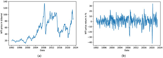
Figure 1. Evolutionof the WTI oil price and its return. (a) Evolution of the WTI oil prices from February 1992 to October 2022. (b) Evolution of the WTI oil prices from February 1992 to October 2022.

Oil prices increased again until July 2014 but fell sharply as the United States shale oil product expanded. From 2016 to 2019, oil prices exhibited relatively stable behavior but dropped dramatically during the COVID-19 pandemic. In recent months, oil prices exhibited an upward trend in response to the war between Russia and Ukraine. Moreover, oil prices showed high levels of volatility from 2006 to 2008, increasing by almost 120%, from $60 to approximately $134 a barrel. Within six months, they decreased by nearly 250% to $39 a barrel by February 2009. Since then, oil prices have substantially oscillated, indicating structural breaks in the industry.

3.2. Estimation Strategies

Before using the price in time series analysis, proceeding to some diagnostic checks, such as the stationarity and autoregressive conditional heteroscedasticity tests, is routine. This study applies different traditional tests to test the stationary nature of oil prices, namely, the augmented Dickey–Fuller test ([47], ADF hereafter). For completeness, we also run the Phillips and Perron (PP) test [48] and the Kwiatkowski–Phillips–Schmidt–Shin (KPSS) test proposed by [49]. In addition, we perform Engle’s autoregressive conditional heteroscedasticity test [45] to test for the presence of volatility clustering or time-varying volatility.

For the specification of the ARIMA and SARIMA models, we follow the authors of [12]’s strategy, which consists of identification, estimation, and diagnostic checking stages. In the identification stage, we determine the autoregressive and moving average orders using the autocorrelation functions (ACF) and the partial autocorrelation functions (PACF) and their corresponding plots (see Figure A1 in the Appendix A.2). For the WTI crude oil price, the figure indicates that the autocorrelations do not die out quickly for the price variable, suggesting nonstationarity. However, the ACF dies out quickly for the percentage change in the price or price return, implying stationarity, as established by the stationarity tests in Table 2. For a moving average process $MA\left(q\right)$, the autocorrelations are zero for $j>q$, and the partial autocorrelations tapper off. The cutoff point for the autocorrelation function is to compare the sample autocorrelations to $\pm \frac{\sqrt{2}}{T}$, where T is the number of observations. For an $AR\left(p\right)$ process, the partial autocorrelations ${\theta }_{ii}=0 for i>p$, and the autocorrelations die out quickly. We also compare the partial autocorrelation function to $\pm \frac{\sqrt{2}}{T}$ to decide about the $AR\left(p\right)$ cutoff. If neither the autocorrelations nor the partial autocorrelations have a cutoff point, then the ARMA model may be appropriate [50].

Table 2. Probabilityvalues for stationarity and ARCH tests for oil price and its return.

Variable	ADF	PP	KPSS	ARCH
Oil price	0.3815	0.4000	0.0100	0.0000
Price return	0.0000	0.0000	0.1000	0.0000

In the empirical part, we split the data into a training set (75%) and a test set (25%). We also augment the FRED-MD data with a dummy representing the 2007–2009 recession (According to the U.S. National Bureau of Economic Research (NBER) website, the recession started in December 2007 and ended in June 2009. See https://www.nber.org/research/data/us-business-cycle-expansions-and-contractions, accessed on 22 April 2023), and a dummy representing the COVID-19 pandemic. We then estimate and use the following models to forecast the WTI oil price:

• Partial least squares model (PLS). We use this model to forecast the WTI oil price and extract a reduced set of components that we use as explanatory variables in subsequent models.
• Ordinary least-squares (OLS) with the most important PLS components as explanatory variables, in addition to recession and COVID-19 dummy variables.
• Autoregressive integrated moving average (ARIMA) with p, d, and q determined by minimizing the Akaike information criterion.
• Autoregressive integrated moving average with the most important PLS components as exogenous variables (ARIMAX1) and the PLS components, in addition to recession and COVID-19 dummy variables as exogenous variables (ARIMAX2).
• Seasonal autoregressive integrated moving average (SARIMA) with p, d, q, P, and Q determined by minimizing the Akaike information criterion.
• Seasonal autoregressive integrated moving average with the most important PLS components as exogenous variables (SARIMAX1) and the PLS components, in addition to recession and COVID-19 dummy variables as exogenous variables (SARIMAX2).
• Autoregressive conditional heteroscedasticity (ARCH) model. Given its wide use for financial data and parsimony, we used ARCH(1).
• The autoregressive conditional heteroscedasticity model with the most important PLS components as exogenous variables (ARCHX(1)).
• The generalized autoregressive conditional heteroscedasticity (GARCH) model. Given its wide use for financial data and parsimony, we used GARCH(1,1).
• The generalized autoregressive conditional heteroscedasticity model with the most important PLS components as exogenous variables (GARCHX(1,1)).

To compare the forecasting performance of each model, we use the mean absolute (MAE), the mean absolute percentage error (MAPE), and the root mean squared error (RMSE) on the out-of-sample observations. Equation (7) gives the expression of each criterion used in model comparison.

$$\begin{array}{c}\hfill \mathrm{MAPE}=\frac{1}{T_{os}}\sum _{t=1}^{T_{os}}\frac{\mid y_t-{\widehat{y}}_t\mid }{\mid y_t\mid }\\ \hfill \mathrm{MAE}=\frac{{\sum }_{t=1}^{T_{os}}\mid y_t-{\widehat{y}}_t\mid }{T_{os}}\\ \hfill \mathrm{RMSE}=\sqrt{\frac{{\sum }_{t=1}^{T_{os}}{\left(y_t-{\widehat{y}}_t\right)}^2}{T_{os}}},\end{array}$$

(7)

where $T_{os}$ is the out-of-sample total number of observations, $y_t$ is the observed WTI oil price, and ${\widehat{y}}_t$ is the forecast WTI oil price.

4. Results

4.1. Time Series Specification and Diagnostic Results

Table 2 shows the p-values of the unit root test result using the ADF, PP, and KPSS tests for the WTI oil price and its return. For the ADF and PP tests, the null hypothesis is the existence of a unit root (the time series is not stationary), while for the KPSS test, the null hypothesis is that the time series is stationary. The p-values indicate that the ADF and PP test statistics fail to reject the null hypothesis for the oil price. The KPSS test also confirms this result, rejecting the null hypothesis of the stationarity of the oil prices. In contrast, the ADF and PP tests reject the null hypothesis for the price return variable, indicating that the oil price is integrated with order one. A similar conclusion is reached using the KPSS test. To avoid spurious regression results, we estimate all of the models using the percentage change in the price (price return) but recover the forecast of the original price series.

Moreover, Table 2 provides the results of Engle’s test, testing the null hypothesis of the absence of conditional heteroscedasticity. The p-values of Engle’s test indicate the presence of autoregressive conditional heteroscedasticity for the WTI oil price and its return.

In selecting the appropriate ARIMA model, we consider the parsimony concept; the authors of [12] argue that parsimonious models produce better forecasts than over-parameterized models. We achieve parsimony by using the Akaike information criterion (AIC) when using the function $auto\_arima$ from the Python package pmdarima [51]. The algorithm returned an ARIMA(3,1,1) as the best model with $AIC=1574.575$. For the seasonal autoregressive moving average model, the algorithm returned a SARIMA(3,1,1)(3,0,1,12) for the seasonal autoregressive moving average.

Moreover, the partial least-squares method reduces the number of explanatory variables and removes the multicollinearity issues inherent in the FRED-MD data, as evidenced in Appendix Table A1. Table 3 gives the cumulative variance and the reduction in the mean squared error of the PLS components. In contrast, Figure 2 provides a graphical representation of Table 3. The results indicate that ten PLS components explain more than 98% of the oil price variation. As the number of components increases, the explained variance increases but very marginally. Consequently, we can use the first ten components as explanatory variables of the oil price variation, that is,

$$p_t={\beta }_0+\sum _{j=1}^{10}{\beta }_{j}Com p_{jt}+{ϵ}_t$$

(8)

Table 3. Cumulative variance explained and the mean squared error reduction by the PLS components.

Components	Cumulative Variance (%)	Mean Squared Error
One component	85.11	151.32
Ten components	98.11	19.31
Fifteen components	98.35	16.70
Twenty components	98.47	15.36
Thirty components	98.55	14.53
Sixty components	98.55	14.33
One hundred components	98.45	14.33

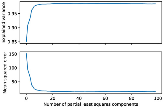
Figure 2. Explained cumulative variance and reduction in the mean squared error and the number of PLS components.

4.2. PLS and OLS Results

4.2.1. PLS Results

The partial least-squares model produced the out-of-sample WTI oil price forecast summarized in Figure 3. The figure shows that the PLS model with ten components successfully forecasts the in-sample WTI oil prices. The out-of-sample forecasts tell a different story, however. The out-of-sample predictions mimic the observed oil price movements, but the prediction values are off, especially during the COVID-19 pandemic. During the pandemic, the PLS model with ten components predicted negative oil prices. Nevertheless, the results indicate that the FRED-MD data, summarized in PLS principal components, is a good predictor tool, but not during extreme events, such as the COVID-19 pandemic.

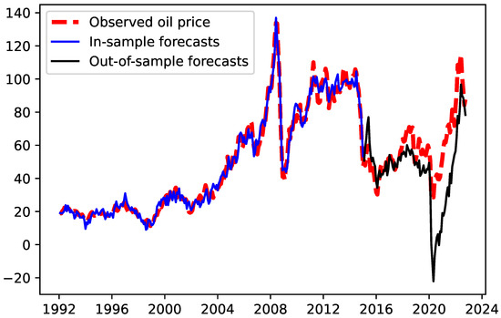
Figure 3. Partial least-squares forecasts with ten components.

4.2.2. OLS Results

To overcome this issue, we augment the ten PLS components with the 2007–2009 financial crisis and COVID-19 pandemic dummy variables and use them as predictors for the WTI oil price. We summarize the results of the least-squares estimation in Table 4. The OLS results show that all ten PLS components are statistically significant in explaining the variation in oil prices. In addition, the 2007–2009 financial crisis had a positive and statistically significant effect on WTI crude oil prices. However, the COVID-19 dummy variable is not statistically significant in explaining the variation in crude oil prices.

Table 4. Lest-squares regression results with 10 PLS components, the 2007–2009 financial crisis, and COVID-19 dummy variables.

Variable	Coefficient	Std. Error	t-Value	p-Value
Intercept	50.9247	0.309	164.803	0.000
PLS component 1	3.8916	0.045	85.602	0.000
PLS component 2	6.1480	0.142	43.183	0.000
PLS component 3	4.6319	0.137	33.795	0.000
PLS component 4	5.1632	0.158	32.689	0.000
PLS component 5	−6.4630	0.260	−24.846	0.000
PLS component 6	−4.1494	0.240	−17.292	0.000
PLS component 7	3.9854	0.301	13.251	0.000
PLS component 8	2.6077	0.467	5.580	0.000
PLS component 9	2.9643	0.420	7.053	0.000
PLS component 10	1.5800	0.307	5.147	0.000
COVID-19	1.6898	1.564	1.080	0.281
2007–2009 financial crisis	4.2152	2.012	2.095	0.037
R-squared:	0.969
Adjusted R-squared:	0.968
F-statistic:	937.3
Prob (F-statistic):	0.000
AIC:	2277
BIC:	2328

Figure 4 displays the in- and out-of-sample forecasts using the OLS model with the PLS components, the COVID-19, and the financial crisis dummy variables. As with PLS, the OLS model successfully fitted the data. However, the out-of-sample forecasts fail to provide high-quality forecasts, especially during high-volatility periods. The OLS model overshoots the price decrease during the COVID-19 pandemic in 2020 and the price increase during the start of the Russia–Ukraine war in 2022.

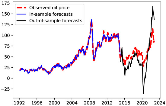
Figure 4. OLS forecasts with ten components, COVID-19, and 2007–2009 financial crisis.

4.3. ARIMA and SARIMA Results

4.3.1. ARIMA Results

As indicated before, the Box–Jenkins [12] identification step yielded the following ARIMA(3,1,1) as the best model:

$$\Delta p_t=\delta +{\theta }_1\Delta p_{t-1}+{\theta }_2\Delta p_{t-2}+{\theta }_3\Delta p_{t-3}+{\alpha }_1{ϵ}_{t-1}+{ϵ}_t.$$

(9)

The maximum likelihood estimation of this model yields the results summarized in Table 5. All of the parameter estimates are statistically significant. The model fitted well the in-sample data, as shown in Figure 5. However, ARIMA(3,1,1) performed poorly in producing accurate out-of-sample forecasts (see Figure 5). The model does not even mimic the price movements as the PLS and OLS did.

Table 5. ARIMA(3,1,1) results.

Variable	Coefficient	Std. Error	t-Value	p-Value
$\Delta p_{t-1}$	1.2564	0.065	19.287	0.000
$\Delta p_{t-2}$	−0.1999	0.088	−2.271	0.023
$\Delta p_{t-3}$	−0.1842	0.047	−3.924	0.000
${ϵ}_{t-1}$	−0.9080	0.047	−19.517	0.000
Log likelihood:	−782.169
AIC:	1574
BIC:	1592

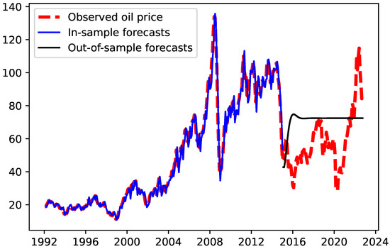
Figure 5. ARIMA(3,1,1) forecasts.

Compared to the PLS and OLS models, the ARIMA model’s poor out-of-sample performance may suggest that the FRED-MD data’s explanatory power, summarized in PLS components, could improve the forecasting accuracy. To explore this possible explanation, we augment the ARIMA(3,1,1) model with ten PLS components and estimate the following equation:

$$\Delta p_t=\delta +{\theta }_1\Delta p_{t-1}+{\theta }_2\Delta p_{t-2}+{\theta }_3\Delta p_{t-3}+{\alpha }_1{ϵ}_{t-1}+{\beta }_0+\sum _{j=1}^{10}{\beta }_{j}Com p_{jt}+{ϵ}_t.$$

(10)

The results of this estimation are summarized in Table 6. The findings indicate that all of the variables included are statistically significant except for the second lag of the price difference.

Table 6. ARIMA(3,1,1) with 10 PLS components regression results.

Variable	Coefficient	Std. Error	t-Value	p-Value
PLS component 1	3.9135	0.074	53.155	0.000
PLS component 2	5.5368	0.280	19.780	0.000
PLS component 3	3.8889	0.232	16.749	0.000
PLS component 4	4.3267	0.287	15.066	0.000
PLS component 5	−6.0491	0.575	−10.522	0.000
PLS component 6	−3.4404	0.463	−7.426	0.000
PLS component 7	3.6362	0.494	7.353	0.000
PLS component 8	4.1290	0.684	6.039	0.000
PLS component 9	3.8184	0.478	7.996	0.000
PLS component 10	1.6372	0.442	3.702	0.000
$\Delta p_{t-1}$	0.7831	0.067	11.771	0.000
$\Delta p_{t-2}$	0.1193	0.080	1.484	0.138
$\Delta p_{t-3}$	−0.1929	0.060	−3.231	0.001
${ϵ}_{t-1}$	−0.9961	0.071	−13.934	0.000
Log likelihood:	−693.196.169
AIC:	1416.392
BIC:	1470.644

In addition, the augmented ARIMA model produces better out-of-sample forecasts than the plain ARIMA model, as indicated by Figure 6. This could indicate the importance of including economic data, such as FRED data, when forecasting commodity prices. However, this model also fails to reproduce the out-of-sample oil prices during high-volatility periods.

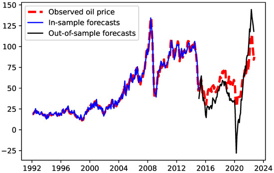
Figure 6. ARIMA(3,1,1) and PLS components forecasts.

To account for the 2007–2009 financial crisis and the COVID-19 pandemic, we added these two events as dummy variables and estimated the following model:

$$\begin{array}{c}\hfill \Delta p_t=\delta +{\theta }_1\Delta p_{t-1}+{\theta }_2\Delta p_{t-2}+{\theta }_3\Delta p_{t-3}+{\alpha }_1{ϵ}_{t-1}+\\ \hfill {\beta }_0+\sum _{j=1}^{10}{\beta }_{j}Com p_{jt}+{\gamma }_{1}fin\_crisi{s}_t+{\gamma }_{2}COVID-{19}_t+{ϵ}_t.\end{array}$$

(11)

The estimation results, summarized in Table 7, show that all PLS components and ARIMA terms are statistically significant at the 1% level, except for the second lag of the price difference, which is significant at the 10% level. The COVID-19 dummy variable has a negative but not statistically significant effect on the oil price. In contrast, the 2007–2009 financial crisis contributed to oil price increases statistically significantly. Nevertheless, adding these two event variables did not improve the forecasting accuracy of the model, as indicated by the negative price forecast during the COVID-19 pandemic period (see Figure 7).

Table 7. ARIMA(3,1,1) with 10 PLS components, COVID-19, and financial crisis regression results.

Variable	Coefficient	Std. Error	t-Value	p-Value
PLS component 1	3.8652	0.110	35.296	0.000
PLS component 2	5.5910	0.362	15.449	0.000
PLS component 3	3.9148	0.254	15.425	0.000
PLS component 4	4.4232	0.282	15.671	0.000
PLS component 5	−5.0474	0.510	−9.905	0.000
PLS component 6	−3.6222	0.438	−8.261	0.000
PLS component 7	3.6609	0.416	8.794	0.000
PLS component 8	3.8124	0.759	5.022	0.000
PLS component 9	4.7275	0.515	9.179	0.000
PLS component 10	2.1798	0.407	5.353	0.000
COVID-19	−0.1028	3.281	−0.031	0.975
2007–2009 financial crisis	2.6813	1.476	1.816	0.069
$\Delta p_{t-1}$	0.8145	0.052	15.771	0.000
$\Delta p_{t-2}$	0.1294	0.070	1.845	0.065
$\Delta p_{t-3}$	−0.1672	0.051	−3.282	0.001
${ϵ}_{t-1}$	−0.9966	0.040	−24.725	0.000
Log likelihood:	−961.427
AIC:	1956.855
BIC:	2023.246

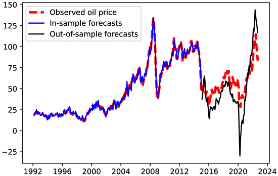
Figure 7. ARIMA(3,1,1) with 10 PLS components, COVID-19, and financial crisis forecasts.

4.3.2. SARIMA Results

To investigate the seasonality of the WTI crude oil prices, we estimate the following seasonal ARIMA model (the orders of SARIMA were chosen using the AIC in the $auto\_arima$ function of the pdmarima Python package.):

$$\begin{array}{c}\hfill \Delta p_t=\delta +{\theta }_1\Delta p_{t-1}+{\theta }_2\Delta p_{t-2}+{\theta }_3\Delta p_{t-3}+{\theta }_{12}\Delta p_{t-12}+{\theta }_{24}\Delta p_{t-24}+\\ \hfill {\theta }_{36}\Delta p_{t-36}{\alpha }_1{ϵ}_{t-1}+{\alpha }_{12}{ϵ}_{t-12}+{ϵ}_t.\end{array}$$

(12)

Though the seasonal lags are statistically significant, as indicated by the results in Table 8, the out-of-sample SARIMA forecasts in Figure 8 show poor performance as the model fails to mimic the price movements, let alone the forecast accuracy.

Table 8. SARIMA(3,1,1)(3,1,1) regression results.

Variable	Coefficient	Std. Error	t-Value	p-Value
$\Delta p_{t-1}$	0.2343	1.717	0.136	0.891
$\Delta p_{t-2}$	0.1933	0.672	0.288	0.774
$\Delta p_{t-3}$	−0.0358	0.232	−0.154	0.877
${ϵ}_{t-1}$	0.1625	1.706	0.095	0.924
$\Delta p_{t-12}$	−0.9886	0.301	−3.283	0.001
$\Delta p_{t-24}$	−0.7137	0.188	−3.793	0.000
$\Delta p_{t-36}$	−0.3692	0.132	−2.793	0.005
${ϵ}_{t-12}$	0.3575	0.294	1.218	0.223
Log likelihood:	−802.728
AIC:	1623.456
BIC:	1636.376

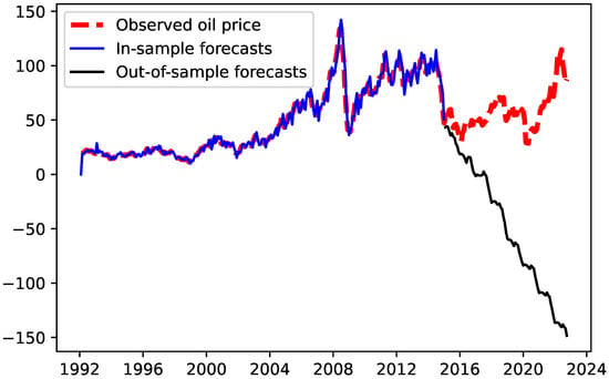
Figure 8. SARIMA(3,1,1)(3,1,1) forecasts.

However, SARIMA forecasts improve when we add the PLS components alone (Figure 9a) and when we augment them with the 2007–2009 financial crisis and the COVID-19 dummy variables (Figure 9b), at least in terms of mimicking the price movements. In terms of the results of the regressions, most PLS components and seasonal terms are statistically significant (see Table 9). In contrast, the results in Table 10 show the COVID-19 dummy variable is not statistically significant in explaining the variation in oil prices for the sample at hand.

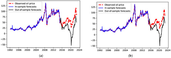
Figure 9. SARIMA with exogenous variables forecasts. (a) SARIMA(3,1,1)(3,1,1) with PLS components forecasts. (b) SARIMA(3,1,1)(3,1,1) with PLS components, COVID-19, and financial crisis forecasts.

Table 9. SARIMA(3,1,1)(3,1,1) with PLS components regression results.

Variable	Coefficient	Std. Error	t-Value	p-Value
PLS component 1	2.3591	2.111	1.118	0.264
PLS component 2	4.6279	1.370	3.378	0.001
PLS component 3	3.4884	1.159	3.011	0.003
PLS component 4	3.3385	0.810	4.122	0.000
PLS component 5	−5.3662	1.851	−2.898	0.004
PLS component 6	−2.3827	1.296	−1.838	0.066
PLS component 7	3.2259	0.961	3.358	0.001
PLS component 8	4.4685	1.703	2.623	0.009
PLS component 9	4.6664	0.936	4.987	0.000
PLS component 10	1.1826	1.041	1.136	0.256
$\Delta p_{t-1}$	−0.0398	2.117	−0.019	0.985
$\Delta p_{t-2}$	0.0860	0.184	0.467	0.641
$\Delta p_{t-3}$	−0.0425	0.199	−0.214	0.830
${ϵ}_{t-1}$	−0.0299	2.135	−0.014	0.989
$\Delta p_{t-12}$	−0.6485	0.317	−2.045	0.041
$\Delta p_{t-24}$	−0.5452	0.193	−2.828	0.005
$\Delta p_{t-36}$	−0.3037	0.151	−2.013	0.044
${ϵ}_{t-12}$	−0.0322	0.329	−0.098	0.922
Log likelihood:	−716.896
AIC:	1471.793
BIC:	1499.068

Table 10. SARIMA(3,1,1)(3,1,1) with PLS components, COVID-19, and financial crisis regression results.

Variable	Coefficient	Std. Error	t-Value	p-Value
PLS component 1	2.4825	1.744	1.423	0.155
PLS component 2	5.3222	1.191	4.469	0.000
PLS component 3	3.3497	0.847	3.953	0.000
PLS component 4	3.8001	0.738	5.150	0.000
PLS component 5	−3.8326	1.475	−2.598	0.009
PLS component 6	−2.2386	1.200	−1.866	0.062
PLS component 7	2.6910	0.915	2.941	0.003
PLS component 8	3.7137	1.576	2.357	0.018
PLS component 9	5.2219	0.798	6.543	0.000
PLS component 10	1.3146	0.905	1.452	0.146
COVID-19	−3.1711	4.709	−0.673	0.501
2007–2009 financial crisis	4.8300	2.481	1.946	0.052
$\Delta p_{t-1}$	−0.0343	0.824	−0.042	0.967
$\Delta p_{t-2}$	0.1506	0.091	1.655	0.098
$\Delta p_{t-3}$	−0.0922	0.140	−0.659	0.510
${ϵ}_{t-1}$	−0.0112	0.839	−0.013	0.989
$\Delta p_{t-12}$	−0.7217	0.346	−2.085	0.037
$\Delta p_{t-24}$	−0.5367	0.226	−2.374	0.018
$\Delta p_{t-36}$	−0.2585	0.154	−1.679	0.093
${ϵ}_{t-12}$	0.0422	0.361	0.117	0.907
Log likelihood:	−995.132
AIC:	2032.263
BIC:	2113.578

4.4. ARCH and GARCH Results

4.4.1. ARCH Results

As seen in Figure 1b, the WTI crude oil price exhibits volatility clustering with periods of high volatility and periods of low volatility. To account for this phenomenon, we estimate augment the ARIMA models to account for conditional variance. For parsimony reasons, we estimated an ARIMA(1,1,0) for the mean and autoregressive conditional heteroscedasticity, ARCH(1), for the variance, that is,

$$\begin{array}{c}\hfill \Delta p_t=\delta +{\theta }_1\Delta p_{t-1}+{ϵ}_t\\ \hfill {\sigma }_t^2=\omega +{\alpha }_1{ϵ}_{t-1}^2+{\eta }_t.\end{array}$$

(13)

The maximum likelihood estimation of Equation (14) produces the results summarized in Table 11. The parameter estimates of the mean and volatility equations are statistically significant at conventional levels. More importantly, the out-of-sample forecasts of the model accurately mimic the observed oil prices even during periods of high instabilities. Figure 10 shows how the ARIMA(1,1,0)-ARCH(1) model predicts future prices with high accuracy. Including the PLS components does not provide a good statistical fit as all of the variables included in the mean and volatility equations are not statistically significant (see Table 12). Nonetheless, the ARIMA(1,1,0)-ARCH(1) with exogenous variables forecasts still produce accurate forecasts, as evidenced in Figure 11.

Table 11. ARIMA(1,1,0) with ARCH(1) regression results.

Mean Equation
Variable	Coefficient	Std. Error	t-Value	p-Value
Intercept	1.0222	0.485	2.109	0.035
$\Delta p_{t-1}$	0.1613	0.064	2.510	0.012
Volatility Equation
Variable	Coefficient	Std. Error	t-Value	p-Value
Intercept	45.6749	5.229	8.735	0.000
${ϵ}_{t-1}^2$	0.2107	0.088	2.400	0.016
Log likelihood:	−935.877
AIC:	1879.75
BIC:	1894.19

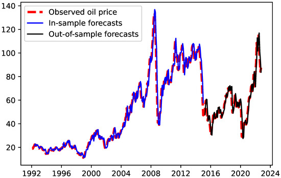
Figure 10. ARIMA(1,1,0) with ARCH(1) forecasts.

Table 12. ARIMA(1,1,0) with PLS components and ARCH(1) regression results.

Mean Equation
Variable	Coefficient	Std. Error	t-Value	p-Value
Intercept	−0.2333	1.633	−0.143	0.886
$\Delta p_{t-1}$	0.1050	0.072	1.451	0.147
PLS component 1	−0.0754	0.121	−0.621	0.534
PLS component 2	0.1796	0.409	0.439	0.661
PLS component 3	0.5069	0.455	1.115	0.265
PLS component 4	0.5770	0.583	0.990	0.322
PLS component 5	0.0908	0.908	0.1000	0.920
PLS component 6	−0.2591	0.683	−0.379	0.704
PLS component 7	0.0867	0.687	0.126	0.900
PLS component 8	0.2325	1.263	0.184	0.854
PLS component 9	0.6985	0.775	0.901	0.368
PLS component 10	0.6087	0.636	0.958	0.338
Volatility Equation
Variable	Coefficient	Std. Error	t-Value	p-Value
Intercept	42.7200	7.611	5.613	0.000
${ϵ}_{t-1}^2$	0.2442	0.181	1.348	0.178
Log likelihood:	−930.915
AIC:	1889.83
BIC:	1940.36

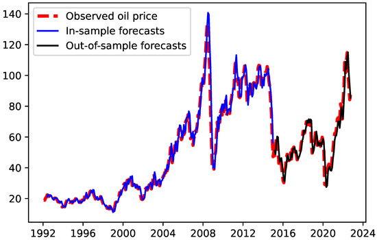
Figure 11. ARIMA(1,1,0) with PLS components and ARCH(1) forecasts.

4.4.2. GARCH Results

We generalized the ARCH model by including past volatility values and estimated the following ARIMA(1,10)-GARCH(1,1):

$$\begin{array}{c}\hfill \Delta p_t=\delta +{\theta }_1\Delta p_{t-1}+{ϵ}_t\\ \hfill {\sigma }_t^2=\omega +{\alpha }_1{ϵ}_{t-1}^2+{\beta }_1{\sigma }_{t-1}^2+{\eta }_t.\end{array}$$

(14)

Table 13 presents the maximum likelihood estimation results. The findings show that ARIMA(1,1,0)-GARCH(1,1) provides an appropriate statistical fit for the data at hand. The lagged price difference in the mean equation and the ARCH and GARCH effects are statistically significant at the 5% level.

Table 13. ARIMA(1,1,0) with GARCH(1,1) regression results.

Mean Equation
Variable	Coefficient	Std. Error	t-Value	p-Value
Intercept	0.5750	0.462	1.245	0.213
$\Delta p_{t-1}$	0.1875	0.065	2.885	0.004
Volatility Equation
Variable	Coefficient	Std. Error	t-Value	p-Value
Intercept	6.0325	5.145	1.172	0.241
${ϵ}_{t-1}^2$	0.1375	0.062	2.211	0.027
${\sigma }_{t-1}^2$	0.7623	0.135	5.665	0.000
Log likelihood:	−929.995
AIC:	1869.99
BIC:	1888.04

Moreover, the model produces accurate out-of-sample forecasts. Figure 12 shows that ARIMA(1,1,0)-GARCH(1,1) accurately predicts the oil price movements and values, even during periods of high volatility, such as the COVID-19 pandemic and the Russia–Ukraine war. This narrative does not change when we add the PLS components to the mean equation. Unlike in the case of ARCH, adding PLS components to the GARCH specification (mean equation) does not impact the statistical significance of ARCH and GARCH effects (see Table 14), nor does it significantly improve the forecasting accuracy of the model (see Figure 13).

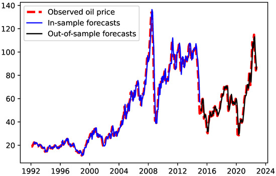
Figure 12. ARIMA(1,1,0) with GARCH(1,1) forecasts.

Table 14. ARIMA(1,1,0) with PLS components and GARCH(1,1) regression results.

Mean Equation
Variable	Coefficient	Std. Error	t-Value	p-Value
Intercept	−1.8532	1.462	−1.267	0.205
$\Delta p_{t-1}$	0.1218	0.068	1.788	0.074
PLS component 1	−0.1412	0.104	−1.355	0.175
PLS component 2	0.6235	0.537	1.161	0.246
PLS component 3	0.8788	0.584	1.506	0.132
PLS component 4	0.9793	0.712	1.376	0.169
PLS component 5	−0.8822	1.089	−0.810	0.418
PLS component 6	−0.3440	0.782	−0.440	0.660
PLS component 7	0.3936	0.755	0.521	0.602
PLS component 8	−0.1077	1.048	−0.103	0.918
PLS component 9	1.3271	0.921	1.441	0.150
PLS component 10	0.5749	0.590	0.975	0.330
Volatility Equation
Variable	Coefficient	Std. Error	t-Value	p-Value
Intercept	6.0498	4.129	1.465	0.143
${ϵ}_{t-1}^2$	0.1292	0.059	2.195	0.028
${\sigma }_{t-1}^2$	0.7623	0.114	6.684	0.000
Log likelihood:	−923.863
AIC:	1877.73
BIC:	1931.87

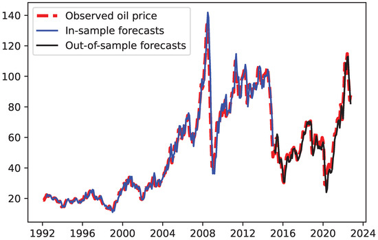
Figure 13. ARIMA(1,1,0) with PLS components and GARCH(1,1) forecasts.

5. Discussion

In this study, we provided alternative models to forecast WTI crude oil prices. We also emphasized the forecasting power of the FRED-MD economic data by estimating models with and without the data. In Table 15, we used the mean absolute percentage error (MAPE), the mean absolute error (MAE), and the root mean squared error (RMSE) to compare alternative models. Our results indicate that the ARIMA(1,1,0)-GARCH(1,1) model outperforms all of the other models in the three criteria. In addition, the models with conditional volatility outperform all of the other models using the three criteria.

Table 15. Forecasting power of alternative models.

Model	MAPE	MAE	RMSE
PLS	0.2585	15.1039	20.2560
OLS	0.3868	21.2806	25.5831
ARIMA(3,1,1)	0.3262	19.0561	22.3438
ARIMAX1(3,1,1)	0.2780	16.2411	19.3317
ARIMAX2(3,1,1)	0.2803	16.3745	19.4875
SARIMA(3,1,1)(3,1,1)	1.8440	107.734	128.3105
SARIMAX1(3,1,1)(3,1,1)	0.5544	32.3907	37.1448
SARIMAX2(3,1,1)(3,1,1)	0.4968	29.0251	33.4761
ARIMA(1,1,0) with ARCH(1)	0.0732	4.2891	5.6916
ARIMAX1(1,1,0) with ARCH(1)	0.0689	4.0384	5.3432
ARIMA(1,1,0) with GARCH(1,1)	0.0605	3.5383	4.6759
ARIMAX1(1,1,0) with GARCH(1,1)	0.0692	4.0589	5.0577

Table 15 shows a significant difference between the ARIMA family models and volatility models, whether we use FRED data or not. Hence, the worst volatility model (in terms of RMSE), namely, ARIMA(1,1,0) with ARCH(1), reduces the forecasting error of ARIMAX1(3,1,1) by more than 70%. This highlights the importance of considering nonlinear time series when studying variables with extreme events.

On the other hand, using FRED-MD data reduces the forecasting error of the corresponding model, except for GARCH. For instance, ARIMA(3,1,1)’s mean absolute percentage error drops from 32.62% to 27.80% when we add the PLS components extracted from FRED-MD data. Moreover, the forecasting error also drops when the PLS components are added to the mean equation of the ARCH(1) model, from 5.69 to 5.34 in terms of root mean squared error.

Regarding previous studies, the authors of [14,38] offer two interesting studies we can use to compare our findings as their goals were to forecast crude oil prices using somewhat similar series. The authors of [14] use ARIMA and SARIMA to forecast crude oil prices in the United States and Europe from January 2017 to September 2021. Their ARIMA and SARIMA models yielded an out-of-sample MAPE of 0.05 and 0.09, respectively. However, their training set included the COVID-19 pandemic period. In contrast, our training set did not include that period, but our conditional variance models (ARCH and GARCH) were successful in producing highly accurate forecasts.

The study by [38] is close to our study regarding the variables and the training set used. The authors used several machine learning models to forecast the WTI crude oil prices, using data from March 1993 to December 2021 (thedata we used was from February 1992 to October 2022) with a test set including the COVID-19 pandemic. In addition, their study used also FRED data besides the economic policy uncertainty data and other financial data. Their change point-adaptive recursive neural network (CP-ADARNN) allows for more reduction in forecast errors compared to our best model. However, one has to be cautious regarding the use of economic data without orthogonalization (partial least-squares or principal components) due to multicollinearity and the consequent risk of overfitting. In contrast, the GARCH model does not present the overfitting risk and is available in most traditional statistical software.

6. Conclusions

In this study, we propose alternative time series models to forecast WTI crude oil prices. We also assess the forecasting power of economic data, namely, FRED data. Our results indicate that when linear models are used (ARIMA and SARIMA), the inclusion of the partial least-squares components extracted from FRED reduces the forecasting error without providing an accurate forecast during high-volatility periods. In contrast, including PLS components from FRED data does not improve the forecasting power volatility models, especially the GARCH model.

Moreover, this paper offers empirical evidence against ignoring conditional volatility in forecasting commodity prices. Even when augmented with economic data spanning all economic activities, linear models, such as ARIMA, provide poor forecasts, especially during extreme events. Our finding highlights the importance of considering nonlinear time series when studying variables with extreme events. In addition, this study’s outcome has practical implications for commodity traders as the GARCH estimation only requires the commodity price.

The findings of this study confirm the use of the generalized autoregressive conditional heteroskedasticity (GARCH) models as a statistical tool that provides high-quality forecasts, not only for the volatility but also for the time series mean. The GARCH model is important because it makes it possible to model financial and economic time series data more precisely. The model effectively captures the key characteristics of the data by taking volatility clustering into consideration. This is critical in crude oil pricing since forecasting depends on precise modeling of volatility. As indicated by Figure 1, the WTI oil prices exhibited volatility clusters during several periods in the 1992–2022 monthly data. Unlike studies, such as [14], our study properly accounts for volatility clustering to capture the important feature of WTI oil prices and produce accurate forecasts.

This study can be improved in several respects. First, future studies may extend the factor models to include global demand, international economic, and geopolitical indicators instead of limiting the analysis to the United States’ economic indicators. In fact, the FRED database only includes variables related to U.S. economic activities. Exploring other variables or indices, such as the ones provided by the Economic Policy Uncertainty (EPU) database, may take into consideration global economic activities.

Second, to palliate linear models’ shortcomings, one of the promising nonlinear modeling techniques is the dynamic model averaging developed by [39]. To allow the forecasting model’s parameters and forecasting accuracy to vary over time, the model integrates the state space approach with the Markov chain process. This modeling approach allows the parameters and the set of explanatory variables to vary over time. To select the model with the highest probability at any given time, the model is frequently accompanied by dynamic model selection (see, for instance, [52]).

Finally, future studies should also consider asymmetric volatility models. Observational evidence shows that negative shocks have different impacts than positive ones on volatility. The use of asymmetric GARCH models, such as the exponential general autoregressive conditional heteroskedastic (EGARCH) model, developed by [53], and the Glosten–Jagannathan–Runkle GARCH(GJR-GARCH) model, developed by [54], are some examples that consider asymmetric volatility.

Appendix A.1

Table A1. Correlation among FRED data variables.

Correlation	Percentage of Variables
More than 0.95	5.55%
More than 0.90	11.06%
More than 0.75	26.07%
More than 0.50	49.46%

Table A1. Correlation among FRED data variables.

Correlation	Percentage of Variables
More than 0.95	5.55%
More than 0.90	11.06%
More than 0.75	26.07%
More than 0.50	49.46%

Appendix A.2

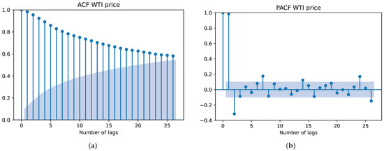
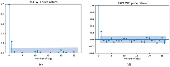
Figure A1. Autocorrelation and partial autocorrelation functions for the WTI oil price and its return. (a) Autocorrelation function for the WTI oil price. (b) Partial autocorrelation function for the WTI oil price. (c) Autocorrelation function for the WTI oil price return. (d) Partial autocorrelation function for the WTI oil price return.

References

- Noreng, O. Crude Power: Politics and the Oil Market; IB Tauris: London, UK, 2006; Volume 21. [Google Scholar]
- Naser, H. Estimating and forecasting the real prices of crude oil: A data rich model using a dynamic model averaging (DMA) approach. Energy Econ. 2016, 56, 75–87. [Google Scholar] [CrossRef]
- Hummels, D. Transportation costs and international trade in the second era of globalization. J. Econ. Perspect. 2007, 21, 131–154. [Google Scholar] [CrossRef]
- Kilian, L.; Lewis, L.T. Does the Fed respond to oil price shocks? Econ. J. 2011, 121, 1047–1072. [Google Scholar] [CrossRef]
- Kilian, L.; Vigfusson, R.J. Are the responses of the US economy asymmetric in energy price increases and decreases? Quant. Econ. 2011, 2, 419–453. [Google Scholar] [CrossRef]
- Abosedra, S.; Baghestani, H. On the predictive accuracy of crude oil futures prices. Energy Policy 2004, 32, 1389–1393. [Google Scholar] [CrossRef]
- Dudley, B. BP statistical review of world energy 2016. In British Petroleum Statistical Review of World Energy; Pureprint Group Limited: East Sussex, UK, 2019. [Google Scholar]
- Belke, A.; Dobnik, F.; Dreger, C. Energy consumption and economic growth: New insights into the cointegration relationship. Energy Econ. 2011, 33, 782–789. [Google Scholar] [CrossRef]
- Kilian, L. Oil Price Volatility: Origins and Effects; Technical Report, WTO Staff Working Paper; World Trade Publications: Geneva, Switzerland, 2010. [Google Scholar]
- Alquist, R.; Kilian, L. What do we learn from the price of crude oil futures? J. Appl. Econom. 2010, 25, 539–573. [Google Scholar] [CrossRef]
- Stevenson, R.A.; Bear, R.M. Commodity futures: Trends or random walks? J. Financ. 1970, 25, 65–81. [Google Scholar] [CrossRef]
- Box, G.E.; Jenkins, G.M. Time Series Analysis: Forecasting and Control; Holden Day: San Francisco, CA, USA, 1976. [Google Scholar]
- Tularam, G.A.; Saeed, T. Oil-price forecasting based on various univariate time-series models. Am. J. Oper. Res. 2016, 6, 226–235. [Google Scholar] [CrossRef]
- Lee, J.Y.; Nguyen, T.T.; Nguyen, H.G.; Lee, J.Y. Towards Predictive Crude Oil Purchase: A Case Study in the USA and Europe. Energies 2022, 15, 4003. [Google Scholar] [CrossRef]
- Mostafa, M.M.; El-Masry, A.A. Oil price forecasting using gene expression programming and artificial neural networks. Econ. Model. 2016, 54, 40–53. [Google Scholar] [CrossRef]
- Álvarez-Díaz, M. Is it possible to accurately forecast the evolution of Brent crude oil prices? An answer based on parametric and nonparametric forecasting methods. Empir. Econ. 2020, 59, 1285–1305. [Google Scholar] [CrossRef]
- Karabiber, O.A.; Xydis, G. Electricity price forecasting in the Danish day-ahead market using the TBATS, ANN and ARIMA methods. Energies 2019, 12, 928. [Google Scholar] [CrossRef]
- Madziwa, L.; Pillalamarry, M.; Chatterjee, S. Gold price forecasting using multivariate stochastic model. Resour. Policy 2022, 76, 102544. [Google Scholar] [CrossRef]
- Purkayastha, D.D. An exposition of the decomposition in a Controlled Autoregressive Integrated Segmented Moving Average (CARISMA) model. Econ. Lett. 1995, 48, 1–7. [Google Scholar] [CrossRef]
- Tseng, F.M.; Tzeng, G.H.; Yu, H.C.; Yuan, B.J. Fuzzy ARIMA model for forecasting the foreign exchange market. Fuzzy Sets Syst. 2001, 118, 9–19. [Google Scholar] [CrossRef]
- Tseng, F.M.; Tzeng, G.H. A fuzzy seasonal ARIMA model for forecasting. Fuzzy Sets Syst. 2002, 126, 367–376. [Google Scholar] [CrossRef]
- Liu, K.; Chen, Y.; Zhang, X. An evaluation of ARFIMA (autoregressive fractional integral moving average) programs. Axioms 2017, 6, 16. [Google Scholar] [CrossRef]
- Brunetti, C.; Gilbert, C.L. Bivariate FIGARCH and fractional cointegration. J. Empir. Financ. 2000, 7, 509–530. [Google Scholar] [CrossRef]
- Serletis, A.; Andreadis, I. Random fractal structures in North American energy markets. Energy Econ. 2004, 26, 389–399. [Google Scholar] [CrossRef]
- Elder, J.; Serletis, A. Long memory in energy futures prices. Rev. Financ. Econ. 2008, 17, 146–155. [Google Scholar] [CrossRef]
- Tabak, B.M.; Cajueiro, D.O. Are the crude oil markets becoming weakly efficient over time? A test for time-varying long-range dependence in prices and volatility. Energy Econ. 2007, 29, 28–36. [Google Scholar] [CrossRef]
- Aloui, C.; Mabrouk, S. Value-at-risk estimations of energy commodities via long-memory, asymmetry and fat-tailed GARCH models. Energy Policy 2010, 38, 2326–2339. [Google Scholar] [CrossRef]
- Agnolucci, P. Volatility in crude oil futures: A comparison of the predictive ability of GARCH and implied volatility models. Energy Econ. 2009, 31, 316–321. [Google Scholar] [CrossRef]
- Kang, S.H.; Kang, S.M.; Yoon, S.M. Forecasting volatility of crude oil markets. Energy Econ. 2009, 31, 119–125. [Google Scholar] [CrossRef]
- Mohammadi, H.; Su, L. International evidence on crude oil price dynamics: Applications of ARIMA-GARCH models. Energy Econ. 2010, 32, 1001–1008. [Google Scholar] [CrossRef]
- Sadorsky, P. Modeling and forecasting petroleum futures volatility. Energy Econ. 2006, 28, 467–488. [Google Scholar] [CrossRef]
- Conrad, C.; Karanasos, M. Dual long memory in inflation dynamics across countries of the Euro area and the link between inflation uncertainty and macroeconomic performance. Stud. Nonlinear Dyn. Econom. 2005, 9. [Google Scholar] [CrossRef]
- Conrad, C.; Karanasos, M. On the inflation-uncertainty hypothesis in the USA, Japan and the UK: A dual long memory approach. Jpn. World Econ. 2005, 17, 327–343. [Google Scholar] [CrossRef]
- Kang, S.H.; Yoon, S.M. Long memory properties in return and volatility: Evidence from the Korean stock market. Phys. A Stat. Mech. Its Appl. 2007, 385, 591–600. [Google Scholar] [CrossRef]
- Kasman, A.; Kasman, S.; Torun, E. Dual long memory property in returns and volatility: Evidence from the CEE countries’ stock markets. Emerg. Mark. Rev. 2009, 10, 122–139. [Google Scholar] [CrossRef]
- McCracken, M.W.; Ng, S. FRED-MD: A monthly database for macroeconomic research. J. Bus. Econ. Stat. 2016, 34, 574–589. [Google Scholar] [CrossRef]
- Baker, S.R.; Bloom, N.; Davis, S.J. Measuring economic policy uncertainty. Q. J. Econ. 2016, 131, 1593–1636. [Google Scholar] [CrossRef]
- Boubaker, S.; Liu, Z.; Zhang, Y. Forecasting oil commodity spot price in a data-rich environment. In Annals of Operations Research; Springer: Berlin/Heidelberg, Germany, 2022; pp. 1–18. [Google Scholar]
- Raftery, A.E.; Kárnỳ, M.; Ettler, P. Online prediction under model uncertainty via dynamic model averaging: Application to a cold rolling mill. Technometrics 2010, 52, 52–66. [Google Scholar] [CrossRef] [PubMed]
- Stock, J.H.; Watson, M.W. Forecasting using principal components from a large number of predictors. J. Am. Stat. Assoc. 2002, 97, 1167–1179. [Google Scholar] [CrossRef]
- Shabri, A.; Samsudin, R. Crude oil price forecasting based on hybridizing wavelet multiple linear regression model, particle swarm optimization techniques, and principal component analysis. Sci. World J. 2014, 2014, 854520. [Google Scholar] [CrossRef]
- Sopipan, N.; Kanjanavajee, W.; Sattayatham, P. Forecasting SET50 index with multiple regression based on principal component analysis. J. Appl. Financ. Bank. 2012, 2, 271. [Google Scholar]
- Binder, K.E.; Pourahmadi, M.; Mjelde, J.W. The role of temporal dependence in factor selection and forecasting oil prices. Empir. Econ. 2020, 58, 1185–1223. [Google Scholar] [CrossRef]
- Franses, P.H.; Van Dijk, D. Non-Linear Time Series Models in Empirical Finance; Cambridge University Press: Cambridge, UK, 2000. [Google Scholar]
- Engle, R.F. Autoregressive conditional heteroscedasticity with estimates of the variance of United Kingdom inflation. In Econometrica: Journal of the Econometric Society; The Econometric Society: Cleveland, OH, USA, 1982; pp. 987–1007. [Google Scholar]
- Bollerslev, T. Generalized autoregressive conditional heteroskedasticity. J. Econom. 1986, 31, 307–327. [Google Scholar] [CrossRef]
- Dickey, D.A.; Fuller, W.A. Likelihood ratio statistics for autoregressive time series with a unit root. In Econometrica: Journal of the Econometric Society; The Econometric Society: Cleveland, OH, USA, 1981; pp. 1057–1072. [Google Scholar]
- Phillips, P.C.; Perron, P. Testing for a unit root in time series regression. Biometrika 1988, 75, 335–346. [Google Scholar] [CrossRef]
- Kwiatkowski, D.; Phillips, P.C.; Schmidt, P.; Shin, Y. Testing the null hypothesis of stationarity against the alternative of a unit root: How sure are we that economic time series have a unit root? J. Econom. 1992, 54, 159–178. [Google Scholar] [CrossRef]
- Griffiths, W.; Hill, R.; Judge, G. Learning and Practicing Econometrics; Wiley: Hoboken, NJ, USA, 1993. [Google Scholar]
- Smith, T. ARIMA Estimators for Python. Available online: http://www.alkaline-ml.com/pmdarima (accessed on 23 April 2017).
- Bork, L.; Møller, S.V. Forecasting house prices in the 50 states using dynamic model averaging and dynamic model selection. Int. J. Forecast. 2015, 31, 63–78. [Google Scholar] [CrossRef]
- Nelson, D.B. Conditional heteroskedasticity in asset returns: A new approach. In Econometrica: Journal of the Econometric Society; The Econometric Society: Cleveland, OH, USA, 1991; pp. 347–370. [Google Scholar]
- Glosten, L.R.; Jagannathan, R.; Runkle, D.E. On the relation between the expected value and the volatility of the nominal excess return on stocks. J. Financ. 1993, 48, 1779–1801. [Google Scholar] [CrossRef]
Disclaimer/Publisher’s Note: The statements, opinions and data contained in all publications are solely those of the individual author(s) and contributor(s) and not of MDPI and/or the editor(s). MDPI and/or the editor(s) disclaim responsibility for any injury to people or property resulting from any ideas, methods, instructions or products referred to in the content. |
© 2023 by the authors. Licensee MDPI, Basel, Switzerland. This article is an open access article distributed under the terms and conditions of the Creative Commons Attribution (CC BY) license (https://creativecommons.org/licenses/by/4.0/).