T-LGBKS: An Interpretable Machine Learning Framework for Electricity Consumption Forecasting

Abstract

Electricity is an essential resource that plays a vital role in modern society, and its demand has increased rapidly alongside industrialization. The accurate forecasting of a country’s electricity demand is crucial for economic development. A high-precision electricity forecasting framework can assist electricity system managers in predicting future demand and production more accurately, thereby effectively planning and scheduling electricity resources and improving the operational efficiency and reliability of the electricity system. To address this issue, this study proposed a hybrid forecasting framework called T-LGBKS, which incorporates TPE-LightGBM, k-nearest neighbor (KNN), and the Shapley additive explanation (SHAP) methods. The T-LGBKS framework was tested using Chinese provincial panel data from 2005 to 2021 and compared with seven other mainstream machine learning models. Our testing demonstrated that the proposed framework outperforms other models, with the highest accuracy ($R^2=0.9732$). This study also analyzed the interpretability of this framework by introducing the SHAP method to reveal the relationship between municipal electricity consumption and socioeconomic characteristics (such as how changes in economic strength, traffic levels, and energy structure affect urban electricity demand). The findings of this study provide guidance for policymakers and assist decision makers in designing and implementing electricity management systems in China.

1. Introduction

Electricity is one of the primary energy sources that ensure the stability and development of the world economy. Ever since the onset of the Second Industrial Revolution, the world has progressively becoming more and more electrified, and electricity has emerged as the cornerstone of every crucial industry and the sustenance of its inhabitants. Modern economic development is closely linked to the demand for electricity. Thus, policymakers in both developed and developing countries emphasize predicting electricity consumption to avoid undesirable forecasting errors. Since electricity consumption prediction is important for the energy sector and the broader economy, developing highly accurate modeling methods is imperative.

China has experienced rapid economic growth and has been the world’s largest energy consumer for over 40 years. In addition, China has been the world’s largest producer and consumer of electricity since 2011 [1]. In recent years, China’s economy has been under downward pressure. Influenced by multiple factors such as a tight electricity supply in some regions, increased demand for electricity in various industries, and the country’s “double control” of energy consumption, the rise in electricity consumption has become more unpredictable [2]. In addition, as the largest carbon emitter, China has committed to achieving a carbon peak by 2030 and carbon neutrality by 2060, which implies a higher cost of electricity production [3]. Hence, it is significant to study the drivers of China’s electricity demand and develop precise forecasting methods [4]. Furthermore, establishing the future electricity market trading mechanism in China requires a scientific and accurate assessment of electricity demand. The accurate forecasting of electricity demand is a prerequisite for the development of a scientific and effective electricity market trading mechanism in China. To this end, various scientific algorithms have been employed for electricity demand forecasting [5]. In the 20th century, researchers in China began exploring electricity forecasting, frequently employing statistical models such as the Kalman filter [6], autoregressive integrated moving average model (ARIMA) [7], and multiple regression model (MLP) [8]. In subsequent years, temporal feature extraction algorithms such as convolutional neural networks (CNNs) and sequence to sequence (seq2seq) [9] transform were introduced to assist these models in improving their forecasting accuracy. In recent times, the emergence of big data technology has led to the widespread adoption of deep learning forecasting models such as artificial neural networks (ANNs), long short-term memory (LSTM), and fuzzy neural networks (FNNs) [10], leading to a significant reduction in electricity forecasting errors.The advancement of accuracy in model predictions is often accompanied by an increase in model complexity. This increase in complexity can result in a poorer explanatory power of the prediction results, which may make it challenging to provide meaningful guidance for managers.

Meanwhile, a precise prediction is pivotal for the establishment and execution of energy policies, specifically electricity tariffs. In order to accurately model electricity consumption in China, this study proposed a hybrid framework incorporating TPE-LightGBM, KNN, and the SHAP methods (T-LGBKS). The results will provide new management insights for urban administrators.

Given the aforementioned arguments, the electricity system necessitates an accurate and interpretable forecasting framework. Therefore, this study proposes an adaptive hybrid machine learning framework, which is applied to the prediction and interpretative analysis of electricity consumption based on multi-source big data. Specifically, the contributions of this study, in comparison with other data-driven approaches, can be summarized as follows:

(1)

This study utilized the RFECV algorithm to automatically select socioeconomic features, thereby reducing the upfront cost and the threshold of use.

(2)

A novel hybrid framework was proposed in this study, which achieves a high accuracy, automatic parameter tuning, and strong interpretability for forecasting urban electricity consumption in China.

(3)

The SHAP method was employed to interpret the input features of the framework. Through the mining of social and economic data, we deeply analyzed the operating mechanism of these indicators affecting urban electricity consumption, providing new insights for relevant managers.

The rest of the paper is organized below. Section 2 presents the study on the factors affecting electricity demand and the typical methods of electricity demand forecasting, and further compares the related research on machine-learning-based approaches. Section 3 proposes constructing an interpretable hybrid framework integrating TPE-LightGBM, KNN, and the SHAP methods (T-LGBKS framework), including the model design at each step and the SHAP method to explain the predicted results of these complex models. Section 4 describes the dataset used in this study and discusses the practical significance of the model by using Chinese provinces as an example. Finally, Section 5 summarizes and suggests future research directions.

2. Literature Review

A comprehensive review of the literature shows that numerous methods have been developed in recent years for forecasting electricity consumption. These models have shifted from traditional linear regression approaches to more sophisticated nonlinear techniques, such as machine learning, gray models, and statistical models. Despite these advances, the performance of existing models may be hindered by a limited availability or outdatedness of data, or even the inadequacy of certain algorithms. Therefore, further improvements are necessary, particularly in developing high-precision forecasting frameworks.

2.1. Factors Influencing Electricity Demand

In recent years, researchers from various countries have conducted extensive theoretical and empirical studies on the factors of electricity consumption. The factors affecting electricity consumption involve many aspects; for instance, the economy, energy, society, policy, and climate. First of all, on the economic side, economic growth would directly increase electricity consumption, as has been confirmed by many researchers [11,12]. Moreover, the secondary industry and its added value had a bidirectional relationship with electricity consumption [13]. Some economists also picked the consumer price index as a driver, demonstrating that CPI growth had a specific inhibitory effect on electricity consumption [14,15]. In addition, the level of economic openness is closely linked to electricity consumption. For instance, the accelerated industrialization process brought about by China’s reform and opening-up policy after 1979 has led to industrial restructuring and increased trade openness, contributing to the growth of electricity consumption. The increase indicates that China’s industrial structure needs to be upgraded [16].

The growth of electricity consumption has played a vital role in fueling China’s economic development [17]. At the same time, this upward trend has also led to a rise in environmental concerns [18]. In the 21st century, environmental pollution and resource scarcity issues have increasingly become a focal point of discussion. The supply of fossil fuels such as oil, coal, and natural gas, as well as energy efficiency, has a significant impact on the electricity supply [19], affecting the demand side of electricity consumption. Electricity tariffs policies are a significant factor that affects electricity demand and can have far-reaching impacts on energy investment and supply and demand. Indirect subsidies in particular have been shown to be likely to negatively affect energy investment, thereby creating ripple effects throughout the electricity supply chain. Therefore, it is imperative that electricity tariffs policies are tailored to the specific market characteristics to support sustainable energy growth [20]. Electricity consumption might also be related to climate, such as cooling in summer and heating in winter [21], but the impact is limited [22]. In addition, China’s electricity reform has further improved the electricity production capacity and generation efficiency [23]. The market-oriented management of the electricity system reduces the elasticity of electricity consumption to a certain extent, lowering the rebound effect and making electricity consumption more responsive to price changes [24], which makes electricity demand expand further.

2.2. Electricity Demand Forecasting Methods

In the twentieth century, researchers in electricity consumption forecasting began trying more complex methods. The accurate forecasting of electricity consumption can lead to a reduction in electricity purchase costs and the optimization of technical processes [25]. Additionally, long-term electricity demand forecasting has been shown to improve socioeconomic efficiency and increase the efficiency of load-planning projects [26,27]. However, long-term forecasting remains a complex task that needs to use factors such as economic growth, weather patterns, and technological advancements. Table 1 lists the critical papers related to electricity forecasting, the main forecasting methods, and a comparison of model accuracy. As illustrated in Table 1, we divided the classical algorithms into time series forecasting and artificial intelligence regression forecasting.

Table 1. The literature on electricity consumption forecasting.

References	Datasets Sources	Model	Data Cleaning Method	RMSE (kw)	MAE (kw)	MAPE (%)	Forecasting Type
Conejo et al. [28]	Electricity price of Spanish power industry in 2002	ARIMA	Wavelet transform	/	/	11.27	short-term
Elamin and Fukushige [29]	The data were obtained from the Tokyo Electric Power Company (TEPCO) website (http://www.tepco.co.jp/forecast/html/download-j.html (accessed on 1 January 2018))	SARIMAX	Logarithms, PACF	31.7	39.2	41.6
Xu and Niimura [30]	PJM spot market price	Multivariate time series	Wavelet transform	6.25	/	/
Panapakidis and Dagoumas [31]	Electricity price from Spanish markets	ANN	Feature selection	/	6.09	/
Wang et al. [32]	Data from an on-campus weather station operated by the University’s Physics Department AND the UF Space Inventory and Allocation System (SPIN)	Random forest	Data transformation Data cleaning	5.12	/	7.5
Wang et al. [33]	Collecting the electricity load data, temperature data, and calendar rules data	SVMD-XGBoost	Cubic spline interpolation method SVMD Feature selection (One-hot encoder, GDBT, Pearson correlation coefficient)	0.118	0.026	4.74
Lu et al. [34]	The raw data come from Data.gov (https://catalog.data.gov (accessed on 1 January 2020))	CEEMDAN- XGBoost	CEEMDAN Normalization	52.8	40.29	5.99
Qiu et al. [35]	From Australian Energy Market Operator (AEMO)	EMD-SVR	ACF Normalization	74.29	/	6.7	medium-term
Li et al. [36]	The data co-sponsored by the Dahang Group, the Yangzhong Hitech Area in Jiangsu province and the   Aliyun company	EEMD-RF	EEMD FFT	22.34	19.42	4.5
Mohandes [37]	1992–1997 hourly electric data load in the Eastern Province in Saudi Arabia	SVR	Removing the outliers, the trend, and the seasonal effect	0.028	/	/
Bouktif et al. [38]	Dataset comes from RTE, which is the electricity transmission system operator of France	LSTM	Data cleansing Normalization Feature scaling	275.6	215.6	/	long-term
Tesfagergis [39]	Collected from the campus of LUT University	Informer	Filling missing values Feature scaling Data splitting	1.45	1.23	49
Bianco et al. [40]	Electricity consumption of Italian statistics by Terna reports	Multiple linear regression models	Data partitioning Difference	<0.2	/	/
Jiang et al. [41]	The electricity demand data from New South Wales (NSW) and Singapore (SG) electric markets	VMD-S-SSASVR	VMD FFT DFT	19.121	14.238	18.5

Time series forecasting usually predicts using periodic regulations and specific trends. In the domain of short and medium-term electricity forecasting, ARIMA models have gained widespread adoption [7]. In particular, Conejo et al. [28] applied ARIMA models combined with wavelet transform techniques to forecast daily electricity prices in 2005. In 2012, Elamin and Fukushige [29] advanced this approach by leveraging the SARIMAX model to perform short-term electricity forecasting with the inclusion of seasonal information. Nevertheless, to further enhance the precision of electricity forecasting, multivariate time series (MTS) forecasting methods that extract temporal features have witnessed rapid development. For instance, Xu and Niimura [30] utilized MTS forecasting to predict short-term electricity demand, demonstrating a superior forecasting performance compared to single time series results. Subsequently, Li et al. [42], Li et al. [43], and Weng [44] developed temporal feature extraction algorithms to extract more feature sequences. Researchers sought to fully exploit these extracted features by combining traditional time series models with artificial neural networks. For instance, Panapakidis and Dagoumas [31] employed clustering analysis and an ANN to forecast electricity prices. Qiu et al. [35] combined empirical mode decomposition algorithms with deep learning models to forecast electricity demand. However, the emergence of big data has rendered simple neural network models inadequate for learning sufficiently.

In recent years, researchers have employed sophisticated neural network layers in combination with time series methods for electricity prediction. Consequently, a dynamic analysis and forecasting method for medium and long-term electricity time series data was developed, relying purely on data-driven methods. Bouktif et al. [38] implemented electricity prediction by constructing a long short-term memory deep learning model, which overcame the issue of vanishing and exploding gradients in standard RNNs and further improved the prediction accuracy. In 2021, Tesfagergis used the transformer model proposed by Google [45] to forecast electricity demand. This model resolved the problem of long training times and the poor performance of long-time series in deep learning network models while exhibiting a relatively consistent performance with the increase in the prediction horizon [39]. However, in electricity forecasting, some indicators, such as GDP, have limited sample sizes, and using advanced network models with multiple hyperparameters may lead to overfitting issues and an inferior performance.

Regression forecasting based on machine learning models is another approach used for electricity forecasting. In 2009, Bianco et al. [40] forecasted the electricity demands of Italy with linear regression methods. Because the relationship between electricity consumption and indicators is often nonlinear, the linear regression model may oversimplify the problem. Mohandes [37] and Jiang et al. [41] utilized a support vector regression (SVR) model, which was optimized to predict electricity demand and demonstrated an excellent performance in capturing nonlinear relationships. However, as the training time increased, it became difficult to identify an appropriate kernel function [46]. Lobato et al. [47] used a single decision tree model to forecast Spanish electricity consumption. They observed that the decision tree model was prone to overfitting due to its instability. Therefore, more and more researchers are using hybridization algorithms with integrated learning, such as random forest (RF) [32,36] and XGBoost [33,34], to make predictions. The results obtained from these hybrid models outperform those obtained from single machine learning models. Unfortunately, integrated learning methods always face overfitting. Moreover, the hyperparameter optimization of XGBoost presents another complex challenge for researchers. The commonly used grid search parameter adjustment method runs very slowly.

Through an extensive exploration of recent top-tier journals in the field of electricity forecasting, this study draws inspiration from two prevailing forecasting approaches and elects to employ regression models for accurate electricity forecasting. Furthermore, to effectively overcome the limitations inherent in existing electricity forecasting models, this research embraces a multi-model compositional ensemble strategy.

2.3. Research Gaps

Throughout the existing literature, numerous scholars have analyzed the influencing factors of electricity consumption and constructed various types of electricity forecasting models that can assist electricity suppliers in rational planning and optimizing energy production, transmission, and distribution to meet demand, enhance efficiency, and reduce energy waste.

However, there are still three minor gaps in the field of electricity consumption forecasting research.

Firstly, most scholars rely on an empirical selection of socio-economic features as input variables but, due to collinearity and correlation among these features, empirical approaches cannot guarantee the operational effectiveness of the models. Moreover, such an approach requires substantial preparatory work and significant human and material resources.

Secondly, there is a delicate trade-off between the interpretability of existing models and their complexity. High-precision models not only pose challenges in parameter tuning but also exhibit a black-box nature, lacking the ability to provide in-depth explanatory analysis.

Lastly, limited literature addresses empirical analyses of energy, microeconomics, transportation capacity, science level, and city size, all of which require further exploration to understand the mechanisms underlying urban electricity consumption.

This study aims to bridge these gaps and serve as a conduit for other researchers while enriching research in this field.

This study proposed a hybrid framework incorporating TPE-LightGBM, KNN, and the SHAP methods (T-LGBKS) to solve the above problems. Specifically, this study introduced the automatic machine learning (Auto-ML) algorithm, which improves the speed of hyper-parameter optimization and provides an automatic feature screening function, significantly reducing the over-fitting problem. In addition, multicollinearity is likely to occur between features in areas such as economic management [48], which may lead to inconsistent analysis results. The tree model adopted in this study was found to be robust to multicollinearity [49]. Additionally, the SHAP algorithm was incorporated into the model to provide an interpretable analysis of the features, thereby unveiling the black-box of machine learning. This feature enables policymakers and decision makers to formulate more effective policies to control future electricity consumption based on the importance of each indicator.

3. Methodology

This section first introduces the models and techniques used in the T-LGBKS framework. Then, some advanced machine learning models as baseline algorithms, widely used in previous research, are also briefly described in order to make the subsequent experiments easier to understand.

3.1. T-LGBKS Framework

3.1.1. TPE Algorithm

To augment the efficacy of the T-LGBKS architecture and expedite the process of hyperparameter optimization, we incorporated the Tree-structured Parzen Estimator (TPE) algorithm. This algorithm facilitates the automatic tuning of hyperparameters in the LightGBM model, thereby improving its performance.

TPE is a sequential model-based optimization algorithm that models $p(x\mid y)$ and $p\left(y\right)$ by transforming the configuration space into non-parametric density distribution. It saves historical evaluation records as an observation domain $H=\left(x_1,f\left(x_1\right),\cdots ,x_n,f\left(x_n\right)\right)$, where $p(x\mid y)$ is defined as Equation (1):

$$p(x\mid y)=\left\{\begin{array}{cc}o\left(x\right),\hfill & \hspace{1em}y<y^{*}\hfill \\ t\left(x\right),\hfill & \hspace{1em}y\ge y^{*}\hfill \end{array}\right.$$

(1)

where $y^{*}$ is the optimal value in the observation domain H, $o\left(x\right)$ denotes the density estimate formed by the observation $\left\{x^i\right\}$ such that the value of the loss is lower than $y^{*}$, and $t\left(x\right)$ represents the density formed by using the remaining observations.

The TPE algorithm is based on the expected improvement (EI) optimization criteria [50,51] for obtaining a new $x^{*}$ and adding it to H, and it is calculated as Equation (2).

$$E{I}_{y^{*}}\left(x\right):={\int }_{-\infty }^{y^{*}}\left(y^{*}-y\right)P(y\mid x)\mathrm{d}y={\int }_{-\infty }^{y^{*}}\left(y^{*}-y\right)\frac{P(x\mid y)P\left(y\right)}{P\left(x\right)}\mathrm{d}y.$$

(2)

By constructing $\gamma =p\left(y<y^{*}\right)$ and $p\left(x\right)={\int }_{R}P(x\mid y)P\left(y\right)\mathrm{d}y=\gamma o\left(x\right)+(1-\gamma )t\left(x\right)$, we have Equation (3):

$$\begin{array}{c}{\int }_{-\infty }^{y^{*}}\left(y^{*}-y\right)·p_M(x\mid y)·p_M\left(y\right)\mathrm{d}y\hfill \\ =o\left(x\right){\int }_{-\infty }^{y^{*}}\left(y^{*}-y\right)·p_M\left(y\right)\mathrm{d}y\hfill \\ =\gamma ·y^{*}·o\left(x\right)-o\left(x\right){\int }_{-\infty }^{y^{*}}{p}_M\left(y\right)\mathrm{d}y\hfill \end{array}$$

(3)

Finally, the value of $E{I}_{y^{*}}\left(x\right)$ is transformed into Equation (4):

$$E{I}_{y^{*}}\left(x\right):=\frac{\gamma y^{*}o\left(x\right)-o\left(x\right){\int }_{-\infty }^{y^{*}}P\left(y\right)\mathrm{d}y}{\gamma o\left(x\right)+(1-\gamma )t\left(x\right)}\propto {\left(\gamma +\frac{t\left(x\right)}{o\left(x\right)}(1-\gamma )\right)}^{-1}$$

(4)

An optimal $x^{*}$ is obtained by maximizing the value of $EI$ in each round of iteration.

3.1.2. Light Gradient Boosting Machine

Introduced in 2017 by Microsoft Research Asia, the light gradient boosting machine (LightGBM) is a state-of-the-art algorithm of the gradient boosting decision tree (GBDT) that has gained wide recognition for its performance [52]. Its versatile applications in finance and big data analytics have been extensively studied [53,54]. Notably, LightGBM outperforms ensemble models such as XGBoost and CatBoost due to its utilization of the gradient-based one-side sampling (GOSS) approach and exclusive feature building (EFB) technique [55]. The estimation function of LightGBM is defined as Equation (5):

$$F_k\left(x\right)=\sum _{k=1}^T{f}_k(x;{\Theta }_k)$$

(5)

where $f_k(x;{\Theta }_k)$ is the regression $subtre{e}_k$, ${\Theta }_k$ is the parameter of the $subtre{e}_k$, and T represents the total number of regression subtrees.

The parameters of the subtree $f_k(x;{\Theta }_k)$ are determined by minimizing the loss function $Loss(y,F_k\left(x\right))$, resulting in Equation (6).

$$\begin{array}{c}{\hat{\Theta }}_k={argmin}_{{\Theta }_k}Loss\left(y,F_k\left(x\right)\right)=\hfill \\ {argmin}_{{\Theta }_k}Loss\left(y,F_{k-1}\left(x\right)+f_k\left(x;{\Theta }_k\right)\right)\hfill \end{array}$$

(6)

where ${\hat{\Theta }}_k$ is the estimate of ${\Theta }_k$.

LightGBM employs GOSS to split the internal nodes, selecting samples with larger gradients (i.e., top $a\times 100\%$) as subset A, whereas the remaining samples with smaller gradients (i.e., $b\times (1-a)\times 100\%$) are randomly selected as subset B. Therefore, there must be $a+b<1$ and $\frac{1-a}{b}>1$, and the samples are split according to the variance gain $V_j\left(d\right)$ on $A\cup B$ as Equation (7):

$$V_j\left(d\right)=\frac{1}{n}\left[\frac{{\left({\sum }_{x_i\in A_p}{g}_i+\frac{1-a}{b}{\sum }_{x_i\in B_p}{g}_i\right)}^2}{n_p^j\left(d\right)}+\frac{{\left({\sum }_{x_i\in A_q}{g}_i+\frac{1-a}{b}{\sum }_{x_i\in B_q}{g}_i\right)}^2}{n_q^j\left(d\right)}\right]$$

(7)

where $A_p=\left\{x_i\in A:x_{ij}\le d\right\}$, $A_q=\left\{x_i\in A:x_{ij}>d\right\}$, $B_p=\left\{x_i\in B:x_{ij}\le d\right\}$, $B_q=\left\{x_i\in B:x_{ij}>d\right\}$, and $g_i$ denotes the negative gradients of the loss function for the LightGBM outputs in each iteration.

EFB is another technique used by LightGBM to improve its performance. It is a lossless method that reduces the dimensions of features by grouping those with a high degree of mutual exclusivity, thereby reducing memory consumption [56].

We included LightGBM into the T-LGBKS framework because of its performance. Furthermore, the TPE algorithm was employed to optimize its intricate combination of hyperparameters, resulting in the TPE-LightGBM model.

3.1.3. KNN Algorithm

KNN is a widely studied and applied non-parametric, instance-based, and lazy algorithm in data mining and artificial intelligence [57,58]. KNN is effective in clustering based on feature similarity between cities and learning information from neighboring cities for prediction. The prediction task using KNN can be divided into the following five steps.

• Step 1: Calculate the distances between the city to be predicted and the remaining cities in the high-dimensional feature space.
• Step 2: Incrementally sort the remaining cities based on their distances in the feature space.
• Step 3: Select K cities with the smallest distances, and assign different weights to each of these K cities based on the reciprocal of their distances.
• Step 4: Obtain the output value for the prediction city by taking the weighted average of the output values of the K selected cities based on the weights obtained in Step 3.
• Step 5: Repeat Steps 1 to 4 until all cities have been predicted.

In the T-LGBKS framework, we applied the Euclidean distance as the distance formula for the KNN algorithm as it is one of the commonly used distance metrics in data mining and machine learning. The performance of the KNN algorithm is influenced by two key factors, namely the value of K and the choice of distance metric. In our framework, we used the Euclidean distance formula, expressed mathematically as Equation (8).

$$\mathrm{d}(x,y)=\sqrt{{\left(x_1-y_1\right)}^2+{\left(x_2-y_2\right)}^2+\dots +{\left(x_n-y_n\right)}^2}=\sqrt{\sum _{i=1}^n{\left(x_i-y_i\right)}^2}$$

(8)

The principle of the KNN algorithm is shown in Figure 1, where the yellow points represent the sample cities to be predicted and the three subplots correspond to the cases of $K=2$, 3, and 4, respectively.

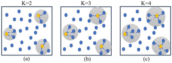
Figure 1. Visualization of KNN. (a) Visualization at K value of 2. (b) Visualization at K value of 3. (c) Visualization at K value of 4.

3.1.4. Shapley Additive Explanation

Interpretability is becoming increasingly important as machine learning algorithms are applied in decision-making contexts. In particular, policymakers often require explanations of how models arrived at their predictions. To meet this need, the T-LGBKS framework uses the SHAP method to interpret each input variable [59]. The SHAP method provides insights into how each variable contributes to the model’s output and can help policymakers to better understand the relationship between socioeconomic characteristics and municipal electricity demand.

Let F denote the complete set of input features and let $S(S\subseteq F)$ represent a subset of features. The approach involves training two models, $f_{S\cup \left\{i\right\}}\left(x_{S\cup \left\{i\right\}}\right)$ and $f_S\left(x_S\right)$, where $featur{e}_i$ is the feature whose impact is to be assessed. The model $f_{S\cup \left\{i\right\}}\left(x_{S\cup \left\{i\right\}}\right)$ is trained using $featur{e}_i$ as one of its inputs, whereas $f_S\left(x_S\right)$ is trained without $featur{e}_i$. Here, $x_{S\cup \left\{i\right\}}$ and $x_S$ represent input feature vectors. The Shapley value of $featur{e}_i$ can be calculated for each possible subset $S\subseteq F\backslash \left\{i\right\}$ as Equation (9):

$${\varphi }_i=\sum _{S\subseteq F\backslash \left\{i\right\}}\frac{\left|S\right|!\left(\right|F|-|S|-1)!}{\left|F\right|!}\left(f_{S\cup \left\{i\right\}}\right(x_{S\cup \left\{i\right\}})-f_S\left(x_S\right))$$

(9)

The computational complexity of Equation (9) increases exponentially with the number of features, which leads to a significant decrease in computational speed. To address this challenge, Lundberg et al. [60] introduced a more efficient approach called Tree SHAP, which can compute the SHAP values in a computationally tractable manner. This approach significantly improves the computational efficiency of the SHAP method, enabling its application in scenarios with many features.

The SHAP method combines optimal assignment with local interpretation using the classical Shapley values, enabling the user to understand how individual features affect the predictive model. Thus, the SHAP interaction value can be calculated as the difference between the Shapley value with $featur{e}_i$ and the Shapley value without $featur{e}_j$ as Equation (10).

$$\begin{array}{cc}\hfill {\varphi }_{i,j}=& \sum _{S\subseteq F\backslash \{i,j\}}\frac{\left|S\right|!\left(\right|F|-|S|-2)!}{\left|F\right|!}\left(f_{S\cup \{i,j\}}\right(x_{S\cup \{i,j\}}\left)\right)\hfill \\ & -f_{S\cup \left\{i\right\}}\left(x_{S\cup \left\{i\right\}}\right)-f_{S\cup \left\{j\right\}}\left(x_{S\cup \left\{j\right\}}\right)-f_S(x_S))\hfill \end{array}$$

(10)

3.1.5. T-LGBKS Framework Process

In this study, we proposed an interpretable hybrid framework, T-LGBKS, which integrates TPE-LightGBM, KNN, and the SHAP methods. The T-LGBKS framework combines the strengths of these algorithms by leveraging both the characteristics of the city itself and the information from similar cities, resulting in the high-precision forecasting of municipal electricity consumption. Furthermore, the SHAP method was incorporated into the machine learning models to provide insights into how the T-LGBKS framework makes decisions, predicts, and performs operations. This interpretability aspect of the T-LGBKS framework can help decision makers to decide better based on the provided information.

The model comprises two main components: data processing and model training. The data processing component consists of three sequential steps, namely padding and scaling, features selection, and splitting the dataset. The model training process encompasses two stages: (1) models pre-training and (2) prediction and analysis. The two stages are implemented as follows.

Stage 1: Models pre-training. The T-LGBKS framework requires the pre-training of the TPE-KNN and TPE-LightGBM models, which proceeds in a three-step process:

Step 1:

Specify the parameters space of the model (KNN or LightGBM);

Step 2:

Optimize the model hyperparameters using 10-fold cross-validation with the TPE algorithm;

Step 3:

Determine whether the optimal parameters are obtained. If not, proceed to Step 2; otherwise, save the optimal model.

Stage 2: Prediction and analysis. This stage builds upon the foundation laid in the first stage. It encompasses two tasks, namely model fusion and SHAP interpretability analysis, which can be further subdivided into the following three steps:

Step 1:

Obtain the KNN model and LightGBM model with optimal parameters from Stage 1, denoted as $K_{opt}$ and $Lg{b}_{opt}$, respectively;

Step 2:

Fuse the $K_{opt}$ and $Lg{b}_{opt}$ models, automatically adjusting the weight factors using the TPE algorithm.

Step 3:

Employ the SHAP algorithm within the T-LGBKS framework to interpret the $Lg{b}_{opt}$ model, thereby comprehending the inner workings of the model’s decision process.

The model fusion in Stage 2 is carried out through bagging. To make the best use of the neighbor information, the $K_{opt}$ nearest neighbors of each sample $x_i([x_{i,1},\cdots ,x_{i,K_{opt}}])$ are stored in ${\mathit{X}}_{\mathit{i}}$, and $x_i$ is also stored in ${\mathit{X}}_{\mathit{i}}$ after prediction using $Lg{b}_{opt}$, i.e., ${\mathit{X}}_{\mathit{i}}=[x_i,[x_{i,1},\cdots ,x_{i,K_{opt}}]]$, while these predicted values are stored in ${\mathit{Y}}_{\mathit{i}}$, i.e., ${\mathit{Y}}_{\mathit{i}}=[y_{i,lgb},[y_{i,1},\cdots ,y_{i,K_{opt}}]]$. The inverse of the Euclidean distance between $x_i$ and $[x_{i,1},\cdots ,x_{i,K_{opt}}]$ is stored in the ${\mathit{D}}_{\mathit{i}}$ vector, i.e., ${\mathit{D}}_{\mathit{i}}=[\frac{1}{d_{i,1}},\cdots ,\frac{1}{d_{i,Kopt}}]$. Thus, the predicted output $y_i$ of the $x_i$ through the T-LGBKS framework can be calculated as Equation (11):

$$y_i=\frac{{\omega }_1{y}_{i,lgb}+{\omega }_2{\sum }_{j=1}^{K_{opt}}\frac{\frac{{\omega }_2}{d_{i,j}}}{{\sum }_{k=1}^{K_{opt}}\frac{1}{d_{i,k}}}{y}_{i,j}}{{\omega }_1+{\omega }_2}=\frac{{\mathit{Y}}_{\mathit{i}}\times {[{\omega }_1,{[\frac{{\omega }_2\times {\mathit{D}}_{\mathit{i}}}{Sum({\mathit{D}}_{\mathit{i}})}]}^T]}^T}{{\omega }_1+{\omega }_2}$$

(11)

where ${\omega }_1\in [-1,1], {\omega }_2\in [-1,1], {\omega }_1+{\omega }_2\ne 0$ are parameters of the model that the TPE algorithm can automatically adjust.

The detailed flowchart of the T-LGBKS framework is illustrated in Figure 2.

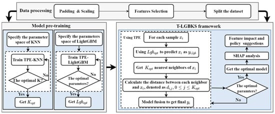
Figure 2. Flowchart of the T-LGBKS framework.

As seen in Figure 2, the framework does not require a manual adjustment of parameters and is an Auto-ML framework, reducing the use threshold. It is also paired with an interpretable analysis, which can effectively guide decision makers and policymakers.

3.2. Baseline Algorithms

To evaluate the effectiveness of the proposed T-LGBKS framework, seven widely adopted machine learning models were selected as baseline models, namely KNN, MLR, SVR, RF, XGBoost, LightGBM, and a deep neural network (DNN). These models will be further elaborated on below.

MLR is considered to be one of the most explanatory models, and its core equation is shown in Equation (12):

$$Y={\beta }_0+{\beta }_1{X}_1+\dots +{\beta }_m{X}_k+ϵ$$

(12)

where Y represents the output value, which, in this study, is the city’s electricity consumption, $X_1,\cdots ,X_m$ are the input features, ${\beta }_0,\cdots ,{\beta }_m$ are regression coefficients, and $ϵ$ denotes the regression residuals. These parameters are usually estimated using the ordinary least squares (OLS) method.

SVR extends the application area of the support vector machine (SVM) to estimate regression problems [61].

The choice of kernel function, i.e., using either the linear kernel, the polynomial kernel, or the RBF kernel, has the largest effect on the performance of SVR. In this study, each of these three methods, denoted as svr_lin, svr_poly, and svr_rbf, were tested.

RF is a well-known ensemble model based on decision trees [62]. It consists of multiple independent classification and regression trees (CARTs). CARTs use the Gini coefficient to select the optimal features and identify the optimal split point of the features. The final output of RF is the average predicted value of all CARTs.

XGBoost is a scalable tree-boosting system [63] known for its high efficiency, flexibility, and portability, and is widely used in various fields such as economics, finance, and management [64]. XGBoost can be viewed as an additive model composed of k base models.

DNN is a branch of artificial neural networks based on a perceptron model [65]. Its structure includes the input, hidden, and output layers. Usually, the hidden layer contains a multi-layer structure.

A summary of the pros and cons of the baseline models is provided in Table 2 below.

Table 2. Pros and cons of baseline models.

Model	Pros	Cons
MLR	Interpretive strength	Data should be linearly correlated
KNN	Data can be non-linear	Long calculation times Poor generalization of models
RF	Ability to handle high-dimensional data Fast operating speed	Prone to over-fitting
XGB	Higher accuracy Ability to automatically handle missing sample values	Prone to over-fitting High complexity of data segmentation
LGB	Higher accuracy Ability to control over-fitting	The feature pre-sorting approach is space-consuming
SVR	Strong model generalization Lower computational complexity	Sensitive to the choice of parameters and kernel functions
DNN	Strong model generalization Higher accuracy	Limited ability to combine features Longer training times

4. Empirical Analysis

In this section, all provinces in the Chinese mainland are selected for the empirical research. The present study employed the monthly indicators as input variables to forecast the electricity consumption for the following month. We first summarized the data used and the data preprocessing method in this study, followed by the metrics used to evaluate the model’s predictive performance. Based on this, we implemented a comparison experiment to verify the performance of the T-LGBKS framework. Finally, we conducted an interpretability analysis of the input features of the SHAP method and proposed policy recommendations. Besides, the code used in this study can refer to Supplementary Materials.

4.1. Study Areas and Data Pre-Process

Before the screening, the data pre-processing of these features was carried out in two steps: padding and scaling. Firstly, for the few missing statistics, this framework used linear interpolation to fill in the data to ensure uniformity in each sample. After that, each feature was subjected to min–max normalization, resulting in Equation (13):

$${\mathit{x}}^{\prime }=\frac{\mathit{x}-min\left(\mathit{x}\right)}{max\left(\mathit{x}\right)-min\left(\mathit{x}\right)}$$

(13)

This study used recursive feature elimination with cross-validation (RFECV, as Algorithm 1) for feature selection. The RFECV algorithm obtains the optimal combination of variables that maximizes the model performance by adding or removing specific feature variables. The pseudo-code of the algorithm is as follows.

Algorithm 1: The RFECV algorithm

Input:  Feature set $\mathit{F}=[f_1,\cdots ,f_m]$; selected subset $\mathit{S}=[S_1,\cdots ,S_n]$   1: Tune/train the LightGBM model on the training set with 10-fold cross-validation using all predictors   2: Calculate variable importance or rankings   3: $\mathit{for}$ Each subset $S_i,i=1,\cdots ,S$ $\mathit{do}$   4:  Keep the $S_i$ most important variables   5:  Tune/train the LightGBM model on the training set with 10-fold cross-validation using all predictors   6:  Recalculate the rankings for each predictor   7: $\mathit{end} \mathit{for}$   8: Calculate the performance profile over the $S_i$   9: Determine the appropriate number of predictors Output:  The optimal feature subset $S_i$

Using the RFECV algorithm, the optimal feature set for the urban electricity consumption forecasting task can be obtained. Table 3 presents the definitions and descriptive statistics of the selected features. Notably, the electricity generation in each province was also selected as an input feature. This is because the widespread adoption of ultra-high-voltage (UHV) technology has normalized the interregional electricity supply, while the reliability of provincial-level electricity generation planning and the existence of China’s complex interprovincial electricity dispatch system contribute to variations between the electricity generation and consumption at the municipal level. For instance, in Beijing, the electricity consumption rate exceeds electricity generation by a factor of two to three, underscoring the magnitude of the disparity created by trans-regional electricity grids. However, the electricity generation data from the previous month can still serve as a reference for the electricity consumption in the current month.

Table 3. Definition of variables and descriptive statistics.

	Definition	Mean	Std. Dec	Minimum	Median	Maximum	Unit
ElectC	Electricity Consumption	169.988	141.254	0.996	126.754	786.710	billion/kWh
GDP	Total Regional GDP	19,671.894	19,803.136	243.090	13,249.781	124,369.672	100 million RMB
SeIGDP	Secondary Industry GDP	8401.223	8656.666	60.520	5386.981	51,775.410	100 million RMB
SRE	Scientific Research Expenditures	40,249.602	57,884.545	34.970	16,134.690	400,220.000	1 million RMB
CPI	Consumer Price Index	102.554	1.740	97.650	102.250	110.090	100 million RMB
NaGC	Natural Gas Consumption	5088.250	4832.996	11.000	3521.667	28,806.000	million/m3
CoalC	Coal Consumption	128.333	100.312	1.828	97.659	513.316	million/ton
RailTV	Rail Transport Volume	118.591	161.997	0.020	64.830	1029.094	million/ton
RoadTV	Road Transport Volume	915.921	712.122	3.460	757.660	3152.230	million/ton
WaterTV	Waterway Transport Volume	163.392	265.352	0.000	52.870	1345.800	million/ton
ElectG	Electricity Generation	168.108	127.814	1.334	134.660	611.520	billion/kWh
UrbP	Urban population	23.854	16.744	0.649	20.805	94.661	million

Finally, this dataset was segmented into training and testing sets, with the training set being used to train the model and testing sets being used to test the performance. To improve data utilization, a 10-fold cross-validation resampling method was used to train the model. The data were divided into four categories: energy (CoalC, NaGC, ElectG), macroeconomics (GDP, SelGDP, CPI), transportation capacity (RailTV, RoadTV, WaterTV), and science level and city size (SRE, UrbP). This data processing framework, which implements several functions such as the automatic padding of data and automatic feature selection, is shown as Figure 3.

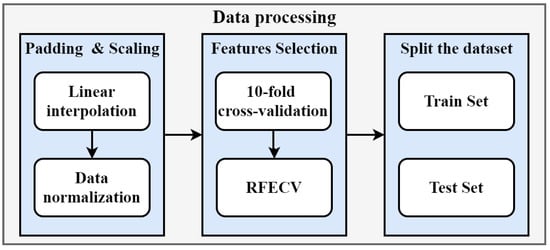
Figure 3. Data processing flow framework.

4.2. Experimental

4.2.1. Evaluation Metrics

This study employed five commonly used evaluation metrics in regression modeling to assess the performance of the proposed algorithms [66], i.e., the coefficient of determination ($R^2$), mean absolute error (MAE), mean square error (MSE), root mean square error (RMSE), and mean absolute percentage error (MAPE).

4.2.2. Experiential Results

This section uses seven regression models to forecast urban electricity consumption. Python 3.9.3 was selected as the programming environment. Furthermore, additional support packages, namely scikit-learn (version 0.24.1) and Tensorflow (version 2.2.2), were selected to calculate and run the ML algorithms. All experiments were repeated ten times based on tests running on a Windows server with dual 2.4 GHz Xeon 8 core processors. All experiment results show the average results of 10 random repetitions for the methods.

Except for the MLR and DNN models, the rest of the baseline algorithms in this study were automatically tuned with parameters by performing 10-fold cross-validation on the training set using the TPE algorithm.

In this study, we constructed a DNN model with a four-layer structure containing two hidden layers. To ensure the model’s performance, truncated Gaussian distributions ($mean=0$, $std=0.05$) were used to initialize hidden layer parameters. Moreover, by introducing the early stop mechanism to alleviate the DNN overfitting, the minimum learning rate was set to 0.003, and the tolerance was set to 20. The Adma algorithm was used as the optimization algorithm, MAE was the loss function, and the maximum number of epochs was set to 300.

The ratio of the training set to the test set was 8:2. The optimal parameters of the TLGBKS framework are listed in Table 4 below, and the optimal parameters of the baseline algorithms can be found in Appendix A.

Table 4. Optimal parameters of the T-LGBKS framework.

Parameters	Value	Definition
$K_{opt}$	3	Number of nearest neighbors
${\omega }_1$	0.75	An adaptive weight of the TPE-LightGBM
${\omega }_2$	0.25	An adaptive weight of the TPE-KNN
boosting_type	‘gbdt’	Boosting algorithm type
n_estimator	637	Number of regressors
subsample	0.862236	For each CART, the proportion of random sampling
max_depth	3	Maximum depth of regressors
colsample_bytree	0.671028	Percentage of columns randomly sampled by each regressor
learning_rate	0.161235	Boosting learning rate

After tuning all models, experiments were conducted on the test set to verify their performance. Following the completion of the models’ predictions, the data were processed by the following inverse normalization equation, after which the evaluation metrics were calculated as Equation (14):

$$\mathit{x}={\mathit{x}}^{\prime }\times \left(max\left({\mathit{x}}^{\prime }\right)-min\left({\mathit{x}}^{\prime }\right)\right)+min\left(\mathit{x}\right)$$

(14)

where ${\mathit{x}}^{\prime }$ is the normalized electricity consumption forecast data and $\mathit{x}$ is the data before normalization.

Table 5 shows the experimental results, with the data in bold representing the optimal values after comparison.

Table 5. Performance comparison in test set.

Model	${\mathit{R}}^2$	MAE	MSE	RMSE	MAPE
MLR	0.9163	22.8105	962.2704	31.0205	38.8897
KNN	0.9434	14.4974	472.5682	21.7386	42.6545
RF	0.9612	13.9546	411.5963	20.2878	9.0453
XGB	0.9612	10.4582	247.6674	15.7375	10.1058
LGB	0.9626	14.0465	497.7796	22.3109	11.2942
svr_rbf	0.9047	36.6011	2151.6162	46.3855	215.5613
svr_lin	0.9077	32.0411	1492.0522	38.6273	102.8659
svr_poly	0.8961	39.8151	2397.2422	48.9616	200.4591
DNN	0.9694	11.3745	301.1564	17.3539	15.9347
T-LGBKS	0.9732	9.5622	213.2972	14.6046	9.0121

The experimental results show that the machine learning model could satisfactorily complete the urban electricity consumption prediction task. The $R^2$ of the XGBoost model and the T-LGBKS framework were even higher than 0.97, indicating that the predicted value was close to the actual value. Meanwhile, Table 5 also demonstrates that the T-LBGK framework proposed in this study outperformed other baseline models, including a deep learning model, and exhibited a superior predictive accuracy in forecasting municipal electricity consumption.

In light of the dynamic nature of the electricity system as a real-time supply–demand system, the unmanageable storage characteristic of electrical energy necessitates meticulous consideration. The overproduction or underproduction of electricity can lead to substantial economic losses for power companies. In light of this crucial consideration, this study introduced an evaluation criterion for electricity prediction models based on the concept of economic loss measurement. The criterion for assessing electricity loss (referred to as loss) was formulated by incorporating the average electricity price (cost), the actual monthly electricity consumption (real), and the predicted monthly electricity consumption (“pred”). Considering the potential benefits of electricity overproduction in addressing sudden contingencies or unexpected demand, the denominator of the criterion was set as the predicted value (pred). The specific definition is provided as Equation (15).

$$loss=cost\times \frac{|real-pred|}{pred}$$

(15)

Assuming $real=100$ and $cost=6.35\times {10}^9$, Table 6 below presents the calculated losses for all electricity prediction models in the current study, considering that all models either overestimate (high) or underestimate (low) the actual values:

Table 6. Measurement of loss in different forecasting models.

Model	MLR	KNN	RF	XGB	LGB
$los{s}_{high}$	$1.18\times {10}^9$	$8.04\times {10}^8$	$7.78\times {10}^8$	$6.01\times {10}^8$	$7.82\times {10}^8$
$los{s}_{low}$	$1.88\times {10}^9$	$1.08\times {10}^9$	$1.03\times {10}^9$	$7.42\times {10}^8$	$1.04\times {10}^9$
Model	svr_rbf	svr_lin	svr_ploy	DNN	T-LGBKS
$los{s}_{high}$	$1.70\times {10}^9$	$1.54\times {10}^9$	$1.81\times {10}^9$	$6.49\times {10}^8$	$5.54\times {10}^8$
$los{s}_{low}$	$3.67\times {10}^9$	$2.99\times {10}^9$	$4.20\times {10}^9$	$8.15\times {10}^8$	$6.71\times {10}^8$

Based on the findings presented in Table 6, it can be conclusively affirmed that the T-LGBKS framework, as proposed in this study, surpasses the baseline models in effectively minimizing economic losses resulting from prediction errors.

From Table 5, it can be observed that the $R^2$ of the MLR model exceeds 0.9, indicating a high level of credibility of the regression equation. Considering the strong interpretability of the regression equation, the regression coefficients help decision makers to gain a quantitative understanding of the importance of the socioeconomic features used in this study. Therefore, the regression coefficients ${\beta }_i,i=1,2,\dots ,11$ are presented in Table 7, and ${\beta }_0=-0.012$. All data are rounded to three decimal places.

Table 7. The regression coefficients of the MLR model.

Feature	$\mathit{\beta }$	Feature	$\mathit{\beta }$	Feature	$\mathit{\beta }$	Feature	$\mathit{\beta }$
GDP	−0.106	CPI	0.008	RailTV	−0.115	ElectG	0.415
SeIGDP	0.322	NaGC	−0.004	RoadTV	−0.031	UrbP	0.148
SRE	0.233	CoalC	0.154	WaterTV	−0.010

In addition, this work also exhibited the prediction performance of the T-LBGKS framework visually. The effect is shown in Figure 4. Due to the large number of cities involved in this study, direct labeling on the figure would lead to readability issues. To address this challenge, we implemented a sample encoding scheme (as shown in Table 8) that corresponds to the x-axis of Figure 4. Specifically, each city has been assigned 17 codes to represent its electricity consumption data over the period of 17 years (from 2005 to 2021), while the y-axis represents the city’s electricity consumption for a given year.

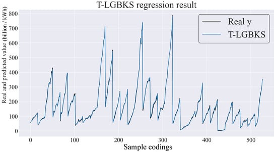
Figure 4. Visualization of regression results for the T-LGBKS framework.

Table 8. Sample encoding for cities and their corresponding years.

Province	Sample Codings	Province	Sample Codings	Province	Sample Codings	Province	Sample Codings
Beijing	1–17	Shanghai	137–153	Hubei	273–289	Yunnan	409–425
Tianjin	18–34	Jiangsu	154–170	Hunan	290–307	Xizang	426–442
Hebei	35–51	Zhejiang	171–187	Guangdong	308–323	Shanxi	443–459
Shanxi	52–68	Anhui	188–204	Guangxi	324–340	Gansu	460–476
Inner Mongolia	69–85	Fujian	205–221	Hainan	341–357	Qinghai	477–493
Liaoning	86–102	Jiangxi	222–238	Chongqing	358–374	Ningxia	494–510
Jilin	103–119	Shandong	239–255	Sichuan	375–391	Xinjiang	511–527
Heilongjiang	120–136	Henan	256–272	Guizhou	392–408

The regression results of the remaining baseline algorithms are visualized in Appendix B for comparison.

The experiment results indicate that random forests, XGBoost, and LightGBM outperformed the other baseline algorithms, highlighting the advantages of the tree-based model. Furthermore, the T-LGBKS framework has been demonstrated to enhance the tree-based models, resulting in a more robust performance.

Figure 5 illustrates the correlation between the anticipated and authentic values of the T-LGBKS framework in the test dataset. As can be observed from the graph, the general predicted and original values cluster closely around the $y=x$ line, and the overall deviation is almost offset. This indicates that the T-LGBKS framework possesses high reliability in the macro-processing of multi-provincial electricity demand forecasting. Additionally, the figure demonstrates that the framework performs well in cities with varying levels of electricity consumption. Notably, there is a slight deviation in the forecast of cities with an electricity consumption range between 200 and 400.

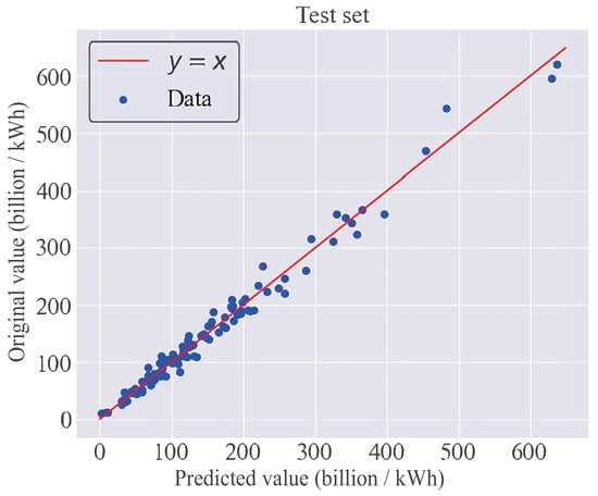
Figure 5. The relationship between the framework predicted value and original value.

Building upon the analysis presented above, the T-LGBKS framework demonstrates notable attributes, including an exceptional accuracy and automated parameter tuning, differentiating it from existing works in the field. These distinguishing features enhance its practical value, making it highly relevant in real-world applications. Such a model is capable of providing accurate electricity demand forecasts, offering decision support to electricity suppliers for optimizing scheduling and resource allocation. By accurately predicting electricity demand, this model assists electricity suppliers in effectively planning and adjusting energy production and transmission plans to meet actual needs and maximize energy utilization efficiency. Additionally, the model’s automatic tuning functionality optimizes model parameters, enhancing the performance and accuracy while reducing the need for manual intervention. This further enhances the reliability and practicality of the model, enabling electricity suppliers to adopt more efficient, economical, and sustainable electricity supply strategies.

4.3. Interpretable Analysis

In this section, we use SHAP interpretability analysis to explain the impact of input features on the LightGBM model in the T-LGBKS framework.

4.3.1. Overall Analysis

Figure 6 is the summary diagram of SHAP. It is sorted by the influence degree of the selected variables on forecasting electricity consumption. The higher the ranking, the more significance the variable has in predicting electricity consumption. When sorting by variables, it can be seen from the diagram that electricity generation was the most essential input variable in this model, which indicates a strong dependence on the long-term relationship between electricity generation and electricity consumption. The output value of the secondary industry was the second characteristic. The sample points with a higher electricity consumption are distributed in the interval with a SHAP value greater than 0, illustrating that an increase in the output value of the secondary industry has a pulling effect on electricity consumption; this is consistent with Danmaraya et al. [13] in that expanding the secondary industry will raise electricity consumption. Followed by gross national product and urban population, the entire economy’s growth will drive the growth of most economic indicators. When the economy is booming, people will increase their electricity consumption, which is consistent with the results of most researchers. At the same time, a growing urban population will quickly stimulate electricity demand. Residential and commercial services, for example, will add to electricity consumption, in line with Günay et al. [22].

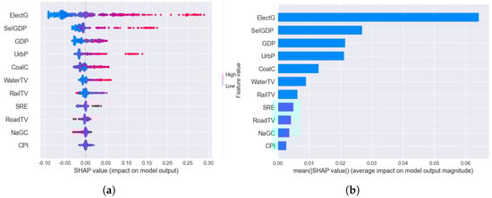
Figure 6. Overall analysis. (a) SHAP overall analysis. (b) Feature importance.

4.3.2. Dependency Analysis

To further verify the relationship between the input variables and the predicted outcomes, we used the SHAP dependency figure to show how the variable values affect the predicted outcomes for each observation in the data set. The dependency figure can describe the major effects of their interactions and individual predictors. We can observe the contribution of each feature that is used to predict scores through global interpretability. We will explore the model outputs in depth from the following four perspectives: energy (CoalC, NaGC, ElectG), macroeconomics (GDP, SelGDP, CPI), transportation capacity (RailTV, RoadTV, WaterTV), and science level and city size (SRE, UrbP).

Firstly, we discuss the impact of energy production and consumption on electricity consumption prediction. Figure 7a shows that, when coal consumption increases (within the range of 0.3–1), the high coal consumption promotes a growth in electricity consumption. From Figure 7b, it can be seen that, when natural gas consumption rises (in the range of 0.3–1), it is inversely proportional to electricity consumption, possibly due to China’s energy structure. China has a high share of coal-fired electricity generation, whereas the share of total natural gas generation is relatively low. As shown in Figure 7c, the electricity generation is proportional to the overall electricity consumption. The rise in electricity generation in different provinces improved the ability to allocate electricity across regions in the short term, and electricity consumption increased.

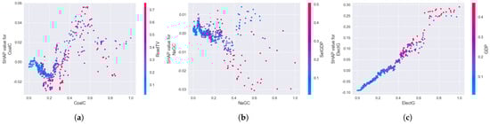
Figure 7. Energy–electricity consumption dependency analysis. (a) Analysis of the dependency of coal consumption and electricity consumption; (b) analysis of the dependency of natural gas consumption and electricity consumption; (c) analysis of the dependency of electricity generation and electricity consumption.

The following section analyzes the macroeconomic impact on electricity consumption forecasting. Figure 8a shows the relationship between changes in GDP and electricity consumption. With a gradual increase in GDP (greater than 0.1), the positive correlation between GDP and electricity consumption becomes stronger. Economic development drives electricity demand. As presented in Figure 8b, the marginal impact of the SelGDP is more significant in the range of (0.3–0.6), which is in accordance with China’s development characteristics. Figure 8c CPI has little effect on electricity consumption. In the range of (0.2–0.4), the growth of CPI will inhibit electricity consumption, likely caused by short-term economic fluctuations such as inflation, which is consistent with the research of Mohammed et al. (2018).

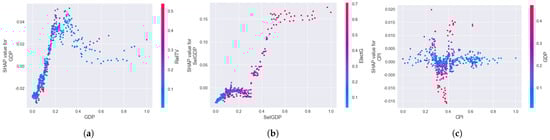
Figure 8. Macroeconomics–electricity consumption dependency analysis. (a) Analysis of the dependency of total regional GDP and electricity consumption; (b) the dependency of secondary industry GDP and electricity consumption; (c) the dependency of consumer price index and electricity consumption.

Then, there is the impact of transportation capacity on electricity consumption forecasting. Low transport levels dampen electricity demand, as shown in Figure 9a. Because China is dominated by thermal electricity generation, important energy sources such as coal require much transport to fulfill electricity demand. With an increase in railway transportation capacity, the growth in electricity consumption will be boosted, as indicated in Figure 9b. When the road transport volume increases (in the range of 0.2–0.4), the increase in road transport volume will increase the electricity demand. In the (0.4–1) range, a high road transport volume has a specific dampening effect on electricity consumption. The reason for this may be that the enhancement of land transport capacity accelerates the mobility of various resources, resulting in resources moving away from the city, thereby dampening electricity demand. As seen in Figure 9c, when the water transport capacity increases (within the range of 0.2–1), the water transport capacity enhances the mobility of resources, thereby increasing electricity demand.

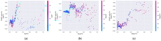
Figure 9. Transportation capacity–electricity consumption dependency analysis. (a) Analysis of the dependency of rail transport volume and electricity consumption; (b) the dependency of road transport volume and electricity consumption; (c) the dependency of water transport volume and electricity consumption.

Finally, we discuss the impact of the level of science and technology and the size of the city on the electricity consumption forecast. The datasets pertaining to scientific research expenditures and urban population have qualities of scientific rigor and global applicability, rendering them suitable for an empirical inquiry into the urban energy sector at the global level. As presented in Figure 10a, a low investment in scientific research undermines electricity consumption. When investment in scientific research rises (in the range of 0.3–1), the level of science increases rapidly, driving economic growth and electricity demand; this suggests a lag in investment in scientific research, corresponding to reality. As Figure 10b demonstrates, when the level of urbanization improves (in the 0.3–1 range) and the electricity demand is rapidly stimulated, again proving the importance of the urban population to electricity consumption.

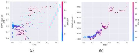
Figure 10. Science level and city size–electricity consumption dependency analysis. (a) Analysis of the dependency of scientific research expenditures and electricity consumption; (b) analysis of the dependency of urban population and electricity consumption.

Most studies in the relevant field rely on multiple linear regression and traditional machine learning models and employ relatively simple indicators with a limited data volume. In contrast, our study utilized more appropriate indicators and a superior machine learning model. Additionally, the use of an SHAP interpretation of visual research results enabled us to derive reliable conclusions for the selected cities. These conclusions can assist decision makers in developing policies and carrying out their usual activities, particularly with regard to energy planning. Nonetheless, there exist certain shortcomings in this study. Owing to limited data availability, we constrained our presentation of China’s electricity consumption forecasts to a monthly basis at the provincial level. In future studies, we aim to improve the frequency of data to enhance the accuracy of our findings.

5. Conclusions

The continuous development of machine learning algorithms has enabled their wide application in various fields, including economics and management. However, the complex mathematical approach within the model makes their operating principles less interpretable. In long-term electricity forecasting for cities, accurate and interpretable predictive models are essential for effective decision making and risk reduction. Therefore, using the tools of visual interpretation to gain insights into the baffling results of machine learning models is of great practical significance.

This study addressed these issues by proposing an interpretable hybrid framework that combines TPE-LightGBM, KNN, and SHAP. We demonstrated this model’s efficient training and successful application in a multi-metric electricity consumption forecasting study. Specifically, we compared the prediction performance of seven baseline models and showed that the T-LGBKS framework outperforms the baseline technique and even traditional deep learning models in electricity forecasting, achieving an MAE of 9.562 and an MAPE of 9.012, a reduction of approximately 30% compared to traditional deep learning models. In addition, other metrics, such as the R², MSE, and RMSE values, were 0.973, 213.297, and 14.604, respectively, all better than the seven baseline models. The forecasting accuracy of the proposed model in this study outperforms the majority of models’ results in the relevant field for long-term electricity demand forecasting.

In this study, we proposed an interpretable hybrid framework combining TPE-LightGBM, KNN, and SHAP to address the limited interpretability of existing models in the field of electricity forecasting. The study analyzed the degree of influence of variables on electricity consumption and identified indicators such as ElectG, SelGDP, GDP, and UrbP as ones with greater influences. Additionally, the dependence of variables on the forecast results was analyzed, revealing a positive correlation between ElectG, CoalC, SelGDP, GDP, UrbP, RailTV, WaterTV, SRE, and electricity consumption, whereas NaGC exhibits a negative relationship. RoadTV was found to inhibit electricity consumption when its value is too low or too high, whereas CPI has little impact on electricity consumption. These results can help administrators to better understand the nonlinear relationships between complex electricity indicators and assist them in developing policies.

Although the T-LGBKS framework proposed in this study performed well, some gaps remain to be filled. Specifically, the framework does not take into account unobservable human and political influences, which may impact electricity consumption. Additionally, the heterogeneity and quantity of the dataset, including the lack of data at higher sampling frequencies, such as weekly or daily, are also limitations. Therefore, our future research plans will involve utilizing data with elevated sampling frequencies to facilitate prediction and scrutinize the impact of data frequency on the model presented in this study. Furthermore, we also plan for this study to collect electricity indicators from cities around the world for forecasting in order to fully verify the generalizability of this framework.

References

- Dudley, B. BP statistical review of world energy. In BP Statistical Review; British Petroleum: London, UK, 2018; p. 00116. [Google Scholar]
- Xie, Y.; Yang, Y.; Wu, L. Power Consumption Forecast of Three Major Industries in China Based on Fractional Grey Model. Axioms 2022, 11, 407. [Google Scholar] [CrossRef]
- Jia, Z.; Lin, B. How to achieve the first step of the carbon-neutrality 2060 target in China: The coal substitution perspective. Energy 2021, 233, 121179. [Google Scholar] [CrossRef]
- Wu, D.; Geng, Y.; Zhang, Y.; Wei, W. Features and drivers of China’s urbanrural household electricity consumption: Evidence from residential survey. J. Clean. Prod. 2022, 365, 132837. [Google Scholar] [CrossRef]
- Klyuev, R.V.; Morgoev, I.D.; Morgoeva, A.D.; Gavrina, O.A.; Martyushev, N.V.; Efremenkov, E.A.; Mengxu, Q. Methods of Forecasting Electric Energy Consumption: A Literature Review. Energies 2022, 15, 8919. [Google Scholar] [CrossRef]
- Takeda, H.; Tamura, Y.; Sato, S. Using the ensemble Kalman filter for electricity load forecasting and analysis. Energy 2016, 104, 184–198. [Google Scholar] [CrossRef]
- Divina, F.; Garcia Torres, M.; Goméz Vela, F.A.; Vazquez Noguera, J.L. A comparative study of time series forecasting methods for short term electric energy consumption prediction in smart buildings. Energies 2019, 12, 1934. [Google Scholar] [CrossRef]
- Alfares, H.K.; Nazeeruddin, M. Electric load forecasting: Literature survey and classification of methods. Int. J. Syst. Sci. 2002, 33, 23–34. [Google Scholar] [CrossRef]
- Zhang, G.; Bai, X.; Wang, Y. Short-time multi-energy load forecasting method based on CNN-Seq2Seq model with attention mechanism. Mach. Learn. Appl. 2021, 5, 100064. [Google Scholar] [CrossRef]
- Almalaq, A.; Edwards, G. A review of deep learning methods applied on load forecasting. In Proceedings of the 2017 16th IEEE International Conference on Machine Learning and Applications (ICMLA), Cancun, Mexico, 18–21 December 2017; pp. 511–516. [Google Scholar]
- Kraft, J.; Kraft, A. On the relationship between energy and GNP. J. Energy Dev. 1978, 3, 401–403. [Google Scholar]
- Zhang, H.; Jiang, X.; Qi, Y.; Hao, Y. How do the industrial structure and international trade affect electricity consumption? New evidence from China. Energy Strategy Rev. 2022, 43, 100904. [Google Scholar] [CrossRef]
- Danmaraya, I.A.; Hassan, S. Electricity consumption and manufacturing sector productivity in Nigeria: An autoregressive distributed lag-bounds testing approach. Int. J. Energy Econ. Policy 2016, 6, 195–201. [Google Scholar]
- Mohammed, N.A. Modelling of unsuppressed electrical demand forecasting in Iraq for long term. Energy 2018, 162, 354–363. [Google Scholar] [CrossRef]
- Molnar, C. Interpretable Machine Learning; Leanpub: Victoria, BC, Canada, 2020. [Google Scholar]
- Zhu, J.; Lin, B. Resource dependence, market-oriented reform, and industrial transformation: Empirical evidence from Chinese cities. Resour. Policy 2022, 78, 102914. [Google Scholar] [CrossRef]
- Du, K.; Lin, B. Understanding the rapid growth of China’s energy consumption: A comprehensive decomposition framework. Energy 2015, 90, 570–577. [Google Scholar] [CrossRef]
- Li, R.; Leung, G.C. Coal consumption and economic growth in China. Energy Policy 2012, 40, 438–443. [Google Scholar] [CrossRef]
- Fang, D.; Hao, P.; Hao, J. Study of the influence mechanism of China’s electricity consumption based on multi-period ST-LMDI model. Energy 2019, 170, 730–743. [Google Scholar] [CrossRef]
- Kök, A.G.; Shang, K.; Yücel, Ş. Impact of electricity pricing policies on renewable energy investments and carbon emissions. Manag. Sci. 2018, 64, 131–148. [Google Scholar] [CrossRef]
- De Felice, M.; Alessandri, A.; Ruti, P.M. Electricity demand forecasting over Italy: Potential benefits using numerical weather prediction models. Electr. Power Syst. Res. 2013, 104, 71–79. [Google Scholar] [CrossRef]
- Günay, M.E. Forecasting annual gross electricity demand by artificial neural networks using predicted values of socio-economic indicators and climatic conditions: Case of Turkey. Energy Policy 2016, 90, 92–101. [Google Scholar] [CrossRef]
- Pollitt, M.; Yang, C.H.; Chen, H.; Energy Policy Research Group. Reforming the Chinese Electricity Supply Sector: Lessons from International Experience; University of Cambridge: Cambridge, UK, 2017. [Google Scholar]
- Meng, M.; Li, X. Evaluating the direct rebound effect of electricity consumption: An empirical analysis of the provincial level in China. Energy 2022, 239, 122135. [Google Scholar] [CrossRef]
- Baczyński, D.; Parol, M. Influence of artificial neural network structure on quality of short-term electric energy consumption forecast. IEE Proc. Gener. Transm. Distrib. 2004, 151, 241–245. [Google Scholar] [CrossRef]
- Maciejowska, K.; Nitka, W.; Weron, T. Day-ahead vs. Intraday—Forecasting the price spread to maximize economic benefits. Energies 2019, 12, 631. [Google Scholar] [CrossRef]
- Ahmad, T.; Zhang, H.; Yan, B. A review on renewable energy and electricity requirement forecasting models for smart grid and buildings. Sustain. Cities Soc. 2020, 55, 102052. [Google Scholar] [CrossRef]
- Conejo, A.J.; Plazas, M.A.; Espinola, R.; Molina, A.B. Day-ahead electricity price forecasting using the wavelet transform and ARIMA models. IEEE Trans. Power Syst. 2005, 20, 1035–1042. [Google Scholar] [CrossRef]
- Elamin, N.; Fukushige, M. Modeling and forecasting hourly electricity demand by SARIMAX with interactions. Energy 2018, 165, 257–268. [Google Scholar] [CrossRef]
- Xu, H.; Niimura, T. Short-term electricity price modeling and forecasting using wavelets and multivariate time series. In Proceedings of the IEEE PES Power Systems Conference and Exposition, New York, NY, USA, 10–13 October 2004; pp. 208–212. [Google Scholar] [CrossRef]
- Panapakidis, I.P.; Dagoumas, A.S. Day-ahead electricity price forecasting via the application of artificial neural network based models. Appl. Energy 2016, 172, 132–151. [Google Scholar] [CrossRef]
- Wang, Z.; Wang, Y.; Zeng, R.; Srinivasan, R.S.; Ahrentzen, S. Random Forest based hourly building energy prediction. Energy Build. 2018, 171, 11–25. [Google Scholar] [CrossRef]
- Wang, Y.; Sun, S.; Chen, X.; Zeng, X.; Kong, Y.; Chen, J.; Wang, T. Short-term load forecasting of industrial customers based on SVMD and XGBoost. Int. J. Electr. Power Energy Syst. 2021, 129, 106830. [Google Scholar] [CrossRef]
- Lu, H.; Cheng, F.; Ma, X.; Hu, G. Short-term prediction of building energy consumption employing an improved extreme gradient boosting model: A case study of an intake tower. Energy 2020, 203, 117756. [Google Scholar] [CrossRef]
- Qiu, X.; Ren, Y.; Suganthan, P.N.; Amaratunga, G.A. Empirical mode decomposition based ensemble deep learning for load demand time series forecasting. Appl. Soft Comput. 2017, 54, 246–255. [Google Scholar] [CrossRef]
- Li, C.; Tao, Y.; Ao, W.; Yang, S.; Bai, Y. Improving forecasting accuracy of daily enterprise electricity consumption using a random forest based on ensemble empirical mode decomposition. Energy 2018, 165, 1220–1227. [Google Scholar] [CrossRef]
- Mohandes, M. Support vector machines for short-term electrical load forecasting. Int. J. Energy Res. 2002, 26, 335–345. [Google Scholar] [CrossRef]
- Bouktif, S.; Fiaz, A.; Ouni, A.; Serhani, M.A. Optimal deep learning lstm model for electric load forecasting using feature selection and genetic algorithm: Comparison with machine learning approaches. Energies 2018, 11, 1636. [Google Scholar] [CrossRef]
- Tesfagergis, A.M. Transformer networks for short-term forecasting of electricity prosumption. In Proceedings of the IEEE Conference on Computer Vision and Pattern Recognition (CVPR), Virtual, 19–25 June 2021; p. 46. [Google Scholar]
- Bianco, V.; Manca, O.; Nardini, S. Electricity consumption forecasting in Italy using linear regression models. Energy 2009, 34, 1413–1421. [Google Scholar] [CrossRef]
- Jiang, P.; Li, R.; Liu, N.; Gao, Y. A novel composite electricity demand forecasting framework by data processing and optimized support vector machine. Appl. Energy 2020, 260, 114243. [Google Scholar] [CrossRef]
- Li, C.; Khan, L.; Prabhakaran, B. Real-time classification of variable length multi-attribute motions. Knowl. Inf. Syst. 2006, 10, 163–183. [Google Scholar] [CrossRef]
- Li, C.; Khan, L.; Prabhakaran, B. Feature Selection for Classification of Variable length Multi-attribute Motions. In Multimedia Data Mining and Knowledge Discovery; Springer: London, UK, 2007; pp. 116–137. [Google Scholar] [CrossRef]
- Weng, X. Classification of Multivariate Time Series Using Supervised Neighborhood Preserving Embedding. In Proceedings of the 2013 25th Chinese Control and Decision Conference (CCDC), Guiyang, China, 25–27 May 2013; pp. 957–961. [Google Scholar] [CrossRef]
- Vaswani, A.; Shazeer, N.; Parmar, N.; Uszkoreit, J.; Jones, L.; Gomez, A.N.; Kaiser, Ł.; Polosukhin, I. Attention is all you need. arXiv 2017, arXiv:1706.03762. [Google Scholar]
- Ray, S. A quick review of machine learning algorithms. In Proceedings of the 2019 International Conference on Machine Learning, Big Data, Cloud and Parallel Computing (COMITCon), Faridabad, India, 14–16 February 2019; pp. 35–39. [Google Scholar] [CrossRef]
- Lobato, E.; Ugedo, A.; Rouco, L.; Echavarren, F.M. Decision trees applied to spanish power systems applications. In Proceedings of the 2006 International Conference on Probabilistic Methods Applied to Power Systems, Stockholm, Sweden, 11–15 June 2006; pp. 1–6. [Google Scholar] [CrossRef]
- Kumari, S.S. Multicollinearity: Estimation and elimination. Int. J. Eng. Sci. 2008, 3, 87–95. [Google Scholar]
- Lindner, T.; Puck, J.; Verbeke, A. Beyond addressing multicollinearity: Robust quantitative analysis and machine learning in international business research. J. Int. Bus. Stud. 2022, 53, 1307–13148. [Google Scholar] [CrossRef]
- Jones, D.R. A taxonomy of global optimization methods based on response surfaces. J. Glob. Optim. 2001, 21, 345–383. [Google Scholar] [CrossRef]
- Bergstra, J.; Bardenet, R.; Bengio, Y.; Kégl, B. Algorithms for hyper-parameter optimization. Adv. Neural Inf. Process. Syst. 2011, 24, 2546–2554. [Google Scholar]
- Ke, G.; Meng, Q.; Finley, T.; Wang, T.; Chen, W.; Ma, W.; Liu, T.Y. Lightgbm: A highly efficient gradient boosting decision tree. Adv. Neural Inf. Process. Syst. 2017, 30, 3149–3157. [Google Scholar] [CrossRef]
- Sun, X.; Liu, M.; Sima, Z. A novel cryptocurrency price trend forecasting model based on LightGBM. Financ. Res. Lett. 2020, 32, 101084. [Google Scholar] [CrossRef]
- Ma, X.; Sha, J.; Wang, D.; Yu, Y.; Yang, Q.; Niu, X. Study on a prediction of P2P network loan default based on the machine learning LightGBM and XGboost algorithms according to different high dimensional data cleaning. Electron. Commer. Res. Appl. 2018, 31, 24–39. [Google Scholar] [CrossRef]
- Al Daoud, E. Comparison between XGBoost, LightGBM and CatBoost using a home credit dataset. Int. J. Comput. Inf. Eng. 2019, 13, 6–10. [Google Scholar] [CrossRef]
- Kotsiantis, S.B. Decision trees: A recent overview. Artif. Intell. Rev. 2013, 39, 261–283. [Google Scholar] [CrossRef]
- Bishop, C.M.; Nasrabadi, N.M. Pattern Recognition And Machine Learning; Springer: New York, NY, USA, 2006; Volume 4, p. 738. [Google Scholar] [CrossRef]
- Song, Y.; Liang, J.; Lu, J.; Zhao, X. An efficient instance selection algorithm for k nearest neighbor regression. Neurocomputing 2017, 251, 26–34. [Google Scholar] [CrossRef]
- Lundberg, S.M.; Lee, S.I. A unified approach to interpreting model predictions. Adv. Neural Inf. Process. Syst. 2017, 30, 4768–4777. [Google Scholar]
- Lundberg, S.M.; Erion, G.; Chen, H.; DeGrave, A.; Prutkin, J.M.; Nair, B.; Katz, R.; Himmelfarb, J.; Bansal, N.; Lee, S.I. From local explanations to global understanding with explainable AI for trees. Nat. Mach. Intell. 2020, 2, 56–67. [Google Scholar] [CrossRef]
- Smola, A.J.; Schölkopf, B. A tutorial on support vector regression. Stat. Comput. 2004, 14, 199–222. [Google Scholar] [CrossRef]
- Breiman, L. Random forests. Mach. Learn. 2001, 45, 5–32. [Google Scholar] [CrossRef]
- Chen, T.; Guestrin, C. Xgboost: A scalable tree boosting system. In Proceedings of the 22nd Acm SIGKDD International Conference on Knowledge Discovery and Data Mining, San Francisco, CA, USA, 13–17 August 2016; pp. 785–794. [Google Scholar] [CrossRef]
- Sagi, O.; Rokach, L. Ensemble learning: A survey. Wiley Interdiscip. Rev. Data Min. Knowl. Discov. 2018, 8, e1249. [Google Scholar] [CrossRef]
- Sze, V.; Chen, Y.H.; Yang, T.J.; Emer, J.S. Efficient processing of deep neural networks: A tutorial and survey. Proc. IEEE 2017, 105, 2295–2329. [Google Scholar] [CrossRef]
- Chicco, D.; Warrens, M.J.; Jurman, G. The coefficient of determination R-squared is more informative than SMAPE, MAE, MAPE, MSE and RMSE in regression analysis evaluation. PeerJ Comput. Sci. 2021, 7, e623. [Google Scholar] [CrossRef]
Disclaimer/Publisher’s Note: The statements, opinions and data contained in all publications are solely those of the individual author(s) and contributor(s) and not of MDPI and/or the editor(s). MDPI and/or the editor(s) disclaim responsibility for any injury to people or property resulting from any ideas, methods, instructions or products referred to in the content. |
© 2023 by the authors. Licensee MDPI, Basel, Switzerland. This article is an open access article distributed under the terms and conditions of the Creative Commons Attribution (CC BY) license (https://creativecommons.org/licenses/by/4.0/).