Article

Capacity Market and Investments in Power Generations: Risk-Averse Decision-Making of Power Producer

1
Institute of Business Sciences, University of Tsukuba, Bunkyo-ku, Tokyo 112-0012, Japan
2
Department of Industrial and Systems Engineering, Tokyo University of Science, Chiba, Noda-shi 278-8510, Japan
*
Author to whom correspondence should be addressed.
Energies 2023, 16(10), 4241; https://doi.org/10.3390/en16104241
Submission received: 31 March 2023 / Revised: 13 May 2023 / Accepted: 16 May 2023 / Published: 22 May 2023
(This article belongs to the Special Issue Forecasting and Risk Management Techniques for Electricity Markets II)

Abstract

:
The penetration of power generations from renewable energy sources into the power market has a significant impact on the capacity factor of existing power generations. This is because power producers cannot recover a capital cost of power generations with high operating cost possibly due to underinvestment. One solution to address this problem includes a capacity mechanism; that is, the capacities of the power generations can be sold through a market or a bilateral contract. Many schemes of the capacity mechanism have been used worldwide. In this study, we examine an investment in a power plant in both the electricity and capacity markets. The effect of investment opportunity on uncertainty and risk aversion is analyzed by a real options approach that is one of analytical methods for investment decisions under uncertainty. The investment timing for the standard energy-only market is compared with that for the capacity market. When the risk averse for the power producer is relatively small, the income in the energy-only market is obtained whereas, when the risk averse is relatively high, the income is gained in both the electricity and capacity markets for the sake of enough profit.

1. Introduction

1.1. Background

Recently, policymakers in the power sector have implemented policies and regulations for solving various problems such as mitigating greenhouse gas emissions and promoting renewable energy. As electricity cannot be economically stored, power producers obtain their profit only when it is delivered to consumers immediately after it is produced via power markets and/or bilateral contracts. Therefore, if producers cannot operate power generations due to the market, policy and regulations, and/or physical conditions for power generations, they might not obtain sufficient profit from selling electricity. Particularly, a capacity factor of power generations with relatively high fuel cost becomes low, and then these are closed due to the operating management depending on the relationship between operating costs and market prices. Meanwhile, the penetration of power generations from renewable energy sources into the power market has a significant impact on the capacity factor of existing power generations. This is because operations of renewable energy sources has become a priority due to their relatively low operating cost, that is, the merit-order effect. Consequently, power producers cannot recover a capital cost of power generations with high operating costs possibly due to underinvestment. This is called the “missing money” problem [1]. European utilities such as RWE, Vattenfall, and E.ON closed or mothballed 21 GW e of gas-fired generation in 2012–2013 although 11 GW e of this generation was less than 10-years-old because of the rise of renewable energy [2]. The penetration of renewable energy into the power market leads to low market prices. Reference [3] indicates that, in the California power market, the price increases slow down due to the high penetration of renewable energy, although the shutdown of nuclear power plants leads to increasing prices.
One of the policies for mitigating this problem includes a capacity mechanism, indicating that power producers can sell their generating capacities kW e through a market of the capacity or via a bilateral contract. Many schemes of the capacity mechanism (e.g., strategic reserve, capacity market, capacity obligation, reliability options, and capacity payments) have been used in many countries. Although the capacity mechanism has a beneficial aspect for the capacity adequacy, some operational capacity adequacy occurs. Even if the revenue is priced adequately through the capacity mechanism, risks such as missing money, cannot be efficiently addressed when it is not perceived by producers. This is the so-called “missing market” problem [4]. Thus, producers should recognize how much effect of risk hedge occurs in the capacity mechanism.
In this study, we consider an investment problem of capacity expansion considering the scheme of capacity mechanisms. We analyze an investment timing for different ratios of selling the capacity. We also compare the investment timing for the standard energy-only market with that for the capacity market.

1.2. Literature Review

There is a growing body of literature that addresses the impact of capacity mechanisms on power market prices and investment decisions for power producers and mitigates the missing money problem by using analytical models [5,6]. Reference [7] evaluates a stability of capacity mechanisms in the presence of uncertainty of the demand growth rate by using a system dynamics model and a Markov Chain Monte Carlo approach. They show that all capacity mechanisms such as capacity payments, operating reserve pricing, and capacity obligation, can contribute to less volatility of power prices and mitigate the shortage. Among these mechanisms, capacity obligation is the most stable both in terms of investment and prices and reduces the market power and offers power producers efficient operating incentives. Reference [8] examines an effect of capacity payment on investment in gas-fired generations under uncertainties of electricity and fuel prices in a real option framework. In a circumstance of this model, they show that capacity payment increases investment opportunity. In cases of capacity payments of 30,000–50,000 EUR/MW p.a., the generations can have positive values even if their capacity factors are low as 5–10%. Thus, they indicate that capacity payment is an important policy for gas-fired generation of a low-capacity factor when shares of renewable energy is high. Reference [9] evaluates a market-wide centralized capacity market and targeted strategic reserves by formulating a game-theoretic market equilibrium model. They find that strategic reserves have significant drawbacks such as an additional investment by replacing the lost flexibility of a contracted capacity. They also show that a centralized capacity market provides a beneficial outcome from both system’s and generator’s perspective. This is because the scheme obtains a suitable reserve margin that avoids energy non-served at the lowest cost and meets the renewable energy target at a lower cost. Reference [10] investigates the robustness and total cost of power generation when the capacity market is adopted, rather than the energy-only market. They analyze a case of the Great Britain market in the framework of a stochastic dynamic model for the capacity investment. They find that the capacity market has a stabilizing effect on unplanned possibilities as no-load of conventional power generations forms the aspects of the cost and price volatility. The introduction of the capacity market leads to an increase in the total cost via payments for the capacity. In the parameter setting, they find that there is an effective region as trade-offs between robustness and costs in the range of reserve margins between 0 and 15%. Reference [11] addresses the dynamics of capacity adequacy and market efficiency with capacity remuneration policy by means of a stochastic simulation model based on the framework of real options. They show that policymakers replace supply security for market prices with payment for consumers when the capacity remuneration mechanism is implemented. They find that when uncertainty affects the growth of electricity demand and power capacity, the capacity market has a beneficial effect in increases in supply security.
The capacity mechanisms have a characteristic of hedging the profit from the energy-only market as forward or option contracts. Thus, the effect of these mechanisms on risk-averse decision-making might become prominent. Reference [12] explores the effect of contracts for the difference, reliability options, and forward capacity market on welfare and investment by using stochastic equilibrium models of risk-averse agents. They find that these contracts are quite effective complements to the energy-only market. However, adding the forward capacity market to the energy-only market can have quite different impacts depending on the extent to which the demand for capacity is calibrated. The contract for the difference and reliability options might also require trade volumes that have never been encountered in power markets. Reference [13] analyzes how the capacity mechanism can address the supply security in power markets by using a system dynamics model that integrates investment and closure decisions. They discuss the energy-only market with a price cap, with and without the capacity mechanisms compared to scarcity pricing in investment decision scenarios with and without risk aversion. In risk-neutral decision-making, the energy-only market with scarcity pricing and the capacity mechanism are two efficient schemes to reach similar levels of load loss. Meanwhile, under risk aversion the capacity mechanism is more effective than scarcity pricing. Reference [14] analyzes the risk aversion of power producers facing an uncertain peak load in the capacity mechanism by using a simulation model based on system dynamics. Particularly, they investigate the impact of the capacity mechanism on the ability to limit shortage and total generation cost, compared to the energy-only market, capacity market, and strategic reserve mechanism. The analytical results indicate that the scheme of the capacity market is the least affected by the degree of risk aversion both with respect to reliability and cost. Therefore, the capacity market is a robust scheme for reliability and cost even if the producers in the market have various forms of risk aversion.
Our work contributes to the literature by exploring how risk-averse decision-making affects investment in power generation and capacity selling in a capacity market. We use the dynamic mean-variance portfolio of [15] by incorporating the real option framework of [16]. Some works focus on investment decisions for risk-averse firms in the real option framework. Reference [17] extends a general model of [16,18] to introduce risk aversion for a constant relative risk aversion utility function in the case where firms face an incomplete market. They show that risk aversion decreases the investment opportunity and detracts the value of investment projects. Reference [19] examines the extent to which operational flexibility in the form of suspension and resumption options with no costs mitigates the effect of risk aversion in the same framework as in [17]. They show how operational flexibility becomes more valuable as risk aversion increases and volatility becomes large. Reference [20] develops a utility-based, regime-switching model to evaluate different technology-adoption strategies under price and technological uncertainty. They find that, when market regimes are asymmetric, larger risk aversion has a non-monotonic impact on the decision to abandon an old market regime and may either increase or decrease the abandonment threshold in contrast with [19].

1.3. Significance and Contribution
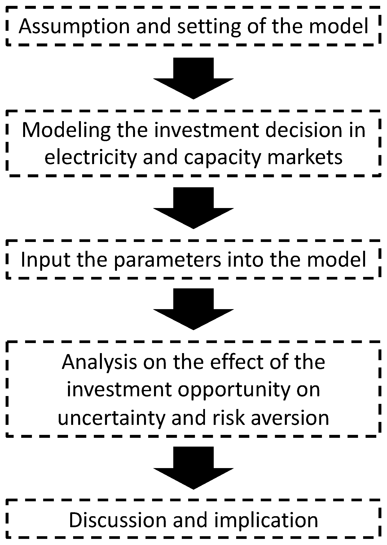
This paper contributes to a growing literature on the relationship between the capacity mechanism and producers’ decision-making under uncertainty. Our main results are as follows.
First, we show that the use of the capacity market depends on risk aversion. When the risk averse for the power producer is relatively small, the income in the energy-only market is obtained. In contrast, when the risk averse is relatively high, the income is gained in both the electricity and capacity markets for the sake of enough profit. Thus, the risk averse power producer might use the capacity market for the risk hedge.
Second, unlike previous papers such as [17,19], an effect of risk aversion on investment decisions is non-monotonic by the existence of the capacity market. When the risk aversion is relatively low, the risk averse power producer increases the investment opportunity in the energy-only market, whereas when the risk aversion is relatively high, they obtain the selling income in both the electricity and capacity market.
The third result is the finding that the relationship between the investment opportunity and the profit rate of the capacity market is ambiguous. When the profit rate is relatively low, that is, a low capacity price compared to electricity (Since the unit of capacity price is different from that of electricity, in this paper suppose that the unit of capacity is converted to the same as electricity), the investment threshold increases with the profit rate. This implies that while the power producers have an incentive to sell the capacity in the market, the investment opportunity decreases because the profit from the electricity market decreases. However meanwhile, when the profit rate is relatively high, the power producers have a large incentive to invest because enough profit from the capacity market can be obtained.
The remainder of this paper is organized as follows. Section 2 develops the model after considering disinvestment and operating flexibility. In Section 3, we derive the optimal policy of the investment in power plants, and examine the effects of parameters on the optimal policy. We use the model to analyze the interaction between equilibrium investments and a renewable energy policy. Figure 1 shows a flowchart of the analysis and discussion in this study. Finally, Section 4 summarizes and concludes the study.

2. Methodology

2.1. Investment Problem to the Power Generator without the Capacity Market

We first consider the investment decision problem to the power generator in the energy-only market (i.e., without the capacity market). As used in previous studies for analytical convenience [21,22,23], we assume that the electricity price follows a geometric Brownian motion (GBM); that is
d P t P t = μ d t + σ d W t
where μ is the instantaneous expected growth rate, σ is the instantaneous volatilities, and W t is a standard Brownian motion (The uncertainty of the electricity price is represented by the GBM, but the model considers no periodicity as a peak hour. If the periodicity is embedded into the model, another stochastic process needs to be used).
Suppose that a single price-taking power producer with a capacity has the perpetual option to invest in a power plant. This study assumes that the power producer sells the total electricity with a capacity factor of 100% that the power producer generates in one power plant, and that there exists no surplus electricity in the power plant.
After the investment at time s, a plant can produce electricity immediately and forever. From this plant, the power producer can sell electricity at exogenous price P t at time t > s . Therefore, the power producer can obtain a discounted accumulated income for selling electricity after the investment as follows:
s e ρ ( t s ) P t d t = P s R
where
R = 0 e ρ t exp μ σ 2 2 t + σ W t d t
and ρ is the discount rate. (3) implies that R fluctuates corresponding to electricity price after the investment time, s. Suppose that the discounted profit from selling electricity is given by
S 1 = B P s R C J ,
where B is a product of a capacity of the power plant and a profit rate, C is the accumulated operating costs including fuel and O&M, and J is an investment cost that is not dependent on investment time. In this study, suppose that the power producer is risk averse, and his/her utility for the discounted profit is the mean-variance type as follows (Although the power utility function has been used in real options analysis [17,19,20], the mean-variance utility is used in this paper because the payoff function is difficult to obtain analytically when the optimal ratio between the energy and capacity markets is derived. Although previous papers of real options have used the power utility in the investment problem, the electricity procurement problem faced by retailers utilizes utility functions with the risk measure as the variance and the value-at-risk as in [24]):
f 1 ( p ) = E S 1 P s = p λ 2 V S 1 P s = p
where λ is a risk-averse coefficient. Since P t follows the GBM, that is, a Markov process, the expected value and the variance of P s R can be obtained as follows (see Appendix A.1):
E P s R P s = p = p E R = p ρ μ ,
V P s R P s = p = p 2 V R = p 2 σ 2 2 ( ρ μ ) ( ρ μ σ 2 2 ) .
Using (6) and (7), the mean-variance utility, f 1 ( p ) , is rewritten as
f 1 ( p ) = γ 2 p 2 + B 0 p I
where
B 0 = B ρ μ ,
I = J + C ,
γ = λ B 0 2 2 η ,
η = ρ μ σ 2 1 2 .
Utility function f 1 ( p ) is a convex quadratic function and has an maximum value at p = p B 0 γ . When the electricity price, p, is high, f 1 ( p ) increases with the income of electricity selling, whereas when the electricity price considerably increases, f 1 ( p ) decreases due to the large risk for price fluctuation. If f 1 ( p ) 0 , the optimal policy is not to invest at all. Therefore, we assume that f 1 ( p ) > 0 . This condition is rewritten as
λ I < η .
Under (13), it is assured that E R < and V R < .
When the present time is t = 0 , the optimal investment problem for the expected utility is formulated by
V 1 ( p ) = sup τ 𝒯 E e ρ τ f 1 ( P τ ) P 0 = p .
𝒯 is a set of all stopping times that are adapted to the filtration generated by a Brownian motion { W t } .

2.2. Investment Problem to the Power Generator with the Capacity Market

In this section, the optimal investment problem in the presence of the capacity market is formulated. The power producer holds the plant by a ratio of r [ 0 , 1 ] and sells electricity in the energy market, whereas the capacity of the remaining 1 r is sold at the investment time in the capacity market. When the electricity price at the investment time, s, is P s , suppose that the profit in the case of selling the full capacity in the market is A P s C (Although there exists no correlation between electricity and capacity prices in any realistic case, we assume the correlation for analytical convenience). Unlike in the case of income for electricity selling, the power producer is not effected by the price fluctuation in the future due to selling the capacity in the market. Since S 1 of (4) is the profit from electricity selling when the power producer holds the power plant, the weighted average profit based on the holding ratio is given by
S 2 = r S 1 + ( 1 r ) ( A P s C J ) = ( B R A ) P s r + A P s I .
Similarly, in Section 2.1, the mean-variance utility for S 2 is calculated as follows:
E S 2 P s = p λ 2 V S 2 P s = p = γ 2 p 2 r 2 + α p r + A p I
where
α = B 0 A .
In this study, we assume that α > 0 because α can be regarded as the risk premium for the price fluctuation in the electricity market. If α 0 , the power producer has no incentive to hold the power plant to sell to the electricity market.
The power producer determines the holding ratio, r, by maximizing (16). Since (16) is a quadratic function for r, the optimal holding ratio is given by
r * ( p ) = 1 , 0 < p p 0 , p 0 p , p > p 0
where p 0 = α γ . When p p 0 , the power producer can obtain the income from electricity selling without selling in the capacity market, whereas when p > p 0 , the power producer tends to sell a portion in the capacity market. The ratio for selling in the capacity market increases with the market price. By substituting r = r * ( p ) into (16), the utility function is given by
f 2 ( p ) = f 1 ( p ) , 0 < p p 0 , f c ( p ) = A p + α 2 2 γ I , p > p 0
where f 1 ( p ) is the utility function without the capacity market. Since f 1 ( p ) is an increasing function for 0 < p p 0 from p 0 < p , f 2 ( p ) is an increasing function for p > 0 . When a capacity market does not exist, the utility function, f 1 ( p ) , decreases due to high price and an increase in the fluctuation risk. However, when the market exists, f 2 ( p ) is an increasing function because the power producer can hedge the fluctuation risk by using the capacity market.
Thus, the optimal investment problem with the capacity market is formulated by
V 2 ( p ) = sup τ 𝒯 E e ρ τ f 2 ( P τ ) P 0 = p .

3. Comparison of Optimal Investment Policies

In Section 3.1, we derive the optimal investment policy of the problems formulated in Section 2. Based on the results, we show comparative statics and investigate in Section 3.2 how model parameters have effects on the optimal policies.

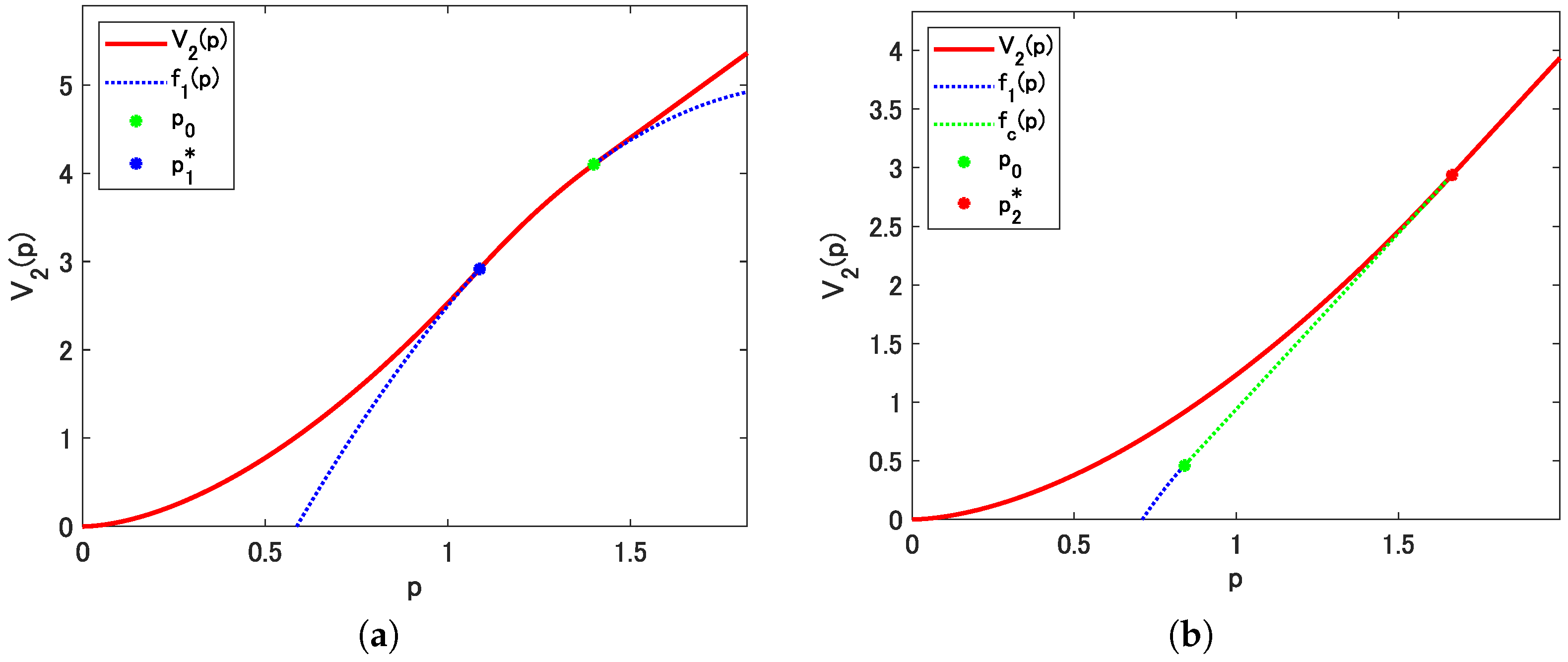
3.1. Optimal Investment Policies

We first derive the optimal policy of the investment problem without the capacity market. As is well-known in the real option analysis, the quadratic equation
σ 2 2 x 2 + ( μ σ 2 2 ) x ρ = 0
has two real solutions, β 1 > 1 and β 2 < 0 , under (13). We define
p 1 * = 2 β 1 I ( β 1 1 + D ) B 0 ,
p 1 = 2 ( β 2 ) I ( 1 β 2 D ) B 0 ,
D = ( β 1 1 ) 2 β 1 ( β 1 2 ) θ ,
D = ( 1 β 2 ) 2 ( β 2 ) ( 2 β 2 ) θ ,
θ = λ I η
where 0 < θ < 1 under (13). Thus, D > 0 and D > 0 .
Theorem 1. 
If the capacity market does not exist, the optimal policy is to invest when p 1 * p p 1 and continue waiting otherwise, where p denotes the electricity price. The value function of this policy is
V 1 ( p ) = f 1 ( p 1 * ) ( p / p 1 * ) β 1 , 0 < p < p 1 * , f 1 ( p ) , p 1 * p p 1 , f 1 ( p 1 ) ( p / p 1 ) β 2 , p > p 1 .
Proof. 
See Appendix A.2. □
As discussed in Section 2.1, utility function f 1 ( p ) in this case is quadratic and concave. Since V 1 ( p ) is smoothly pasted at p = p 1 * and p = p 1 , price p 1 that attains the maximum of f 1 ( p ) satisfies p 1 * < p 1 < p 1 . Value function V 1 ( p ) is increasing for 0 < p < p 1 and decreasing for p > p 1 . It is optimal not to invest both when the electricity price is low and when the price is high enough since it leads to high risk due to a large price fluctuation.
To state the optimal policy when a capacity market exists, we define
p 2 * = β 1 I ( β 1 1 ) A 1 ( 1 A / B 0 ) 2 θ .
Recall that p 0 = α / γ , as defined in Section 2.2.
Theorem 2. 
If there exists a capacity market, the optimal policy is of a threshold type; that is, there exists a threshold price p * such that it is optimal to invest when p p * and continue waiting if p < p * .
(Case 1) If p 2 * p 0 , the threshold price p * = p 1 * , and the value function is given by
V 2 ( p ) = f 1 ( p 1 * ) ( p / p 1 * ) β 1 , 0 < p < p 1 * , f 1 ( p ) , p 1 * p < p 0 , f c ( p ) , p p 0 .
(Case 2) If p 2 * > p 0 , the threshold price p * = p 2 * , and the value function is given by
V 2 ( p ) = f c ( p 2 * ) ( p / p 2 * ) β 1 , 0 < p < p 2 * , f c ( p ) , p p 2 * .
Proof. 
See Appendix A.3. □
In Case 1, if the current electricity price p < p 1 * , it is optimal for the power producer to invest when the price first reaches p 1 * . This policy is the same as in Theorem 1, wherein the capacity market does not exist. In this case, the power producer does not use the capacity market. If the current price p p 1 * , an immediate investment is optimal. The capacity market is utilized only when the current price p > p 0 and 1 p 0 / p of the capacity of the power plant is sold in the capacity market to hedge the risk of price fluctuation in the future. Consequently, the value function V 2 ( p ) is increasing for all p > 0 compared to V 1 ( p ) , which decreases for p > p .
In Case 2, the capacity market is utilized even when the price first reaches to p 2 * and 1 p 0 / p 2 * of the capacity is sold in the capacity market. Value function V 2 ( p ) is increasing for p > 0 as the payoff function f c ( p ) is increasing. From the viewpoint of electricity power producers, a capacity market has a role to hedge risk especially when the price is high.
Figure 2 presents a numerical example where panels (a) and (b) correspond to Cases 1 and 2 in Theorem 2, respectively. We set the parameters as μ = 0.02 , ρ = 0.04 , σ 2 = 0.01 , A = 3 , B 0 = 10 , I = 5 , and λ = 0.15 in panel (a). Panel (b) uses the same set of parameters except for λ = 0.25 . In panel (a), the red solid line represents V 2 ( p ) and the blue dashed line represents f 1 ( p ) . The two marked points in green and blue correspond to p 0 and p 1 * . In panel (b), the red solid line represents V 2 ( p ) , and the blue and green dashed lines represent f 1 ( p ) and f c ( p ) , respectively. The marked points in green and red correspond to p 0 and p 2 * .

3.2. Comparative Statics

As discussed in Section 3.1, the optimal investment policy is of the threshold type when there is a capacity market. In this section, we show the comparative statics of the threshold price in terms of four important parameters: risk aversion coefficient λ , profit ratio of the capacity market A, electricity price volatility σ 2 , and investment cost I. Investigating how these parameters have effects on the threshold price makes it possible to better understand the role of the capacity market in the investment into a new power plant. We also suppose that the remaining parameters μ , ρ , and B (and hence B 0 ) are fixed.
To identify which cases in Theorem 2 occur, we consider
K ( λ , A , σ 2 , I ) = p 2 * p 0 = β 1 { θ ( 1 A / B 0 ) 2 } 2 ( β 1 1 ) ( 1 A / B 0 ) ( A / B 0 ) ,
where θ is given in (26). For presentation simplicity, we will use an abbreviated notation K, rather than K ( λ , A , σ 2 , I ) . Theorem 2 implies that the threshold price p * = p 1 * if K 1 and p * = p 2 * if K > 1 . Moreover, if K > 1 and the power producer makes an investment at the price p = p 2 * , 1 K 1 of the capacity of the plant is sold in the capacity market. To satisfy (13), the domain of λ , σ 2 , and I are limited from above by
λ ¯ = η I , σ 2 ¯ = ρ μ λ I + 1 2 a n d I ¯ = η λ ,
respectively. Since the domain of A is ( 0 , B 0 ) , we denote A ¯ = B 0 .
Theorem 3. 
For any of the parameters x { λ , A , σ 2 , I } , suppose that all other parameters are fixed. Then, there exists a unique x 0 such that K 1 for 0 < x x 0 , and K > 1 for x 0 < x < x ¯ . Moreover, K / x > 0 in the region satisfying K > 0 .
Proof. 
See Appendix A.4. □
Theorem 3 indicates that, when each of the parameters λ , A , σ 2 , or I increases, the threshold price p * switches monotonically from p 1 * to p 2 * . For parameters λ , σ 2 , and I, this is a natural consequence since an increase in these parameters also increases the risk of the power producer, inducing an incentive to hedge risk by using the capacity market. When A increases, the capacity market becomes more attractive so that p * switches from p 1 * to p 2 * .
Theorem 3 also provides an important implication about the utilization of the capacity market. When K > 1 and investment is made at price p = p 2 * , 1 K 1 of the capacity of a plant is sold in the capacity market. From K / x > 0 , the amount of capacity sold in the capacity market increases as each parameter increases. Thus, an increase in these parameters enhances the utilization of the capacity market. When θ goes to 1 (i.e., each of λ , σ 2 or I goes to the upper limit of the domain), the ratio sold in the capacity market tends to
lim θ 1 ( 1 K 1 ) = ( β 1 2 ) ( A / B 0 ) + 2 β 1 ( 2 A / B 0 ) .
Meanwhile, 1 K 1 tends to 1 when A goes to A ¯ , which implies that all of the capacity of the plant is sold in the capacity market if the risk premium contained in the price in the electricity market vanishes.
Subsequently, we further investigate the characteristics of threshold prices. Particularly, we pay attention to whether the threshold price changes monotonically when each parameter increases. The ratio sold in the capacity market is also discussed.

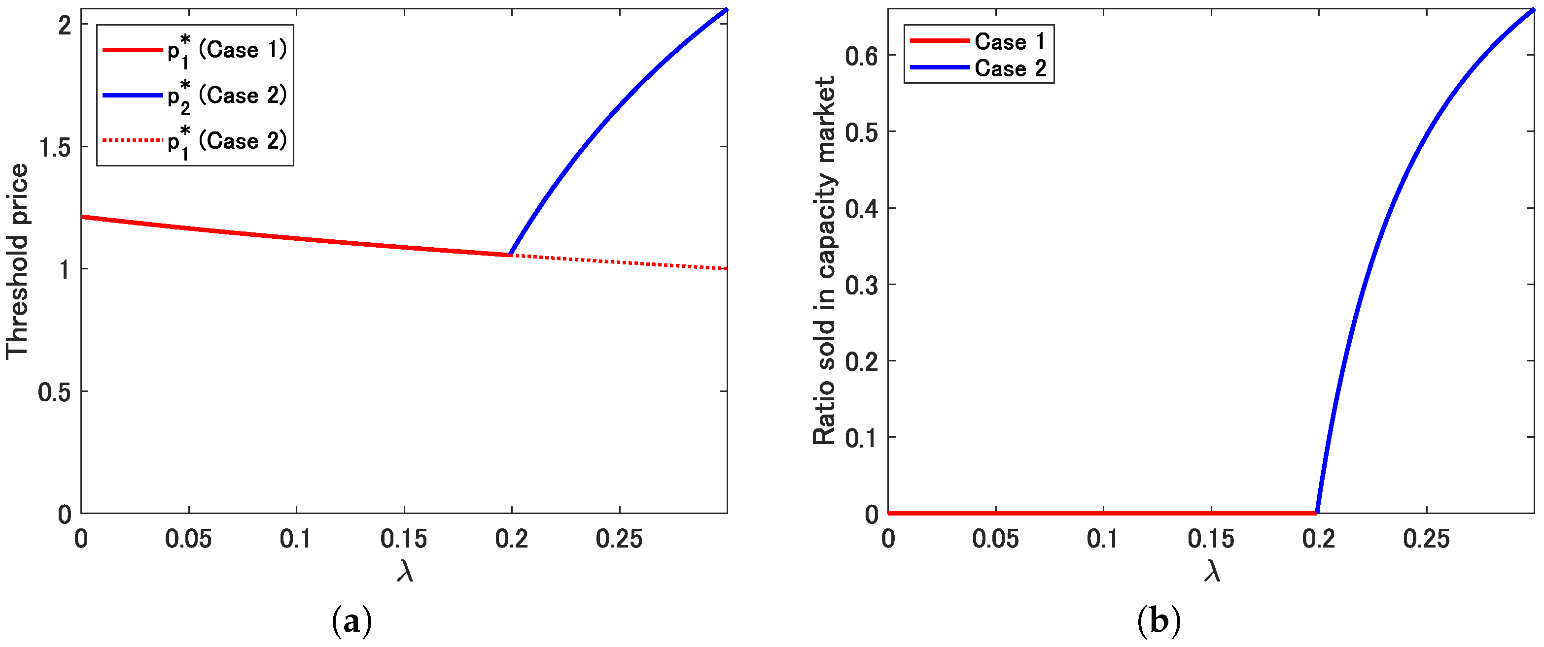
3.2.1. Risk Aversion Coefficient λ

We observe from (22) that p 1 * is a decreasing function of λ if 1 < β 1 < 2 , is constant if β 1 = 2 , and is increasing if β 1 > 2 . Case 1 < β 1 < 2 seems somewhat counter-intuitive since, in many applications of real option analysis, threshold price increases as the investor becomes more risk averse. This may be interpreted in the following manner. The payoff function f 1 ( p ) contains a term γ 2 p 2 , which quadratically decreases as the investment price increases. Meanwhile, the value of waiting increases as p β 1 from (27). Since γ is a linear function of λ , the former effect becomes dominant for large λ when 1 < β 1 < 2 , leading to investment at a lower threshold price.
Unlike p 1 * , (28) shows that p 2 * is an increasing function of λ irrespective of the value of β 1 . This is because a risk-sensitive power producer attempts to obtain a higher payoff by increasing the investment threshold. Although larger p 2 * increases the risk of price fluctuation, this risk can partially be hedged when there is a capacity market.
Figure 3 presents a numerical example that shows threshold price p * as a function of λ . Here and in subsequent numerical examples, we use the same set of parameters in Figure 2b as the base case. In panel (a), red and blue solid lines represent p 1 * and p 2 * , respectively. For comparison, we also plot p 1 * in Case 2 with a red dashed line. Since β 1 = 1.70 < 2 in this case, p 1 * gradually decreases. The threshold price switches from p 1 * to p 2 * at λ 0 = 0.199 and starts to increase rather sharply. As a result, an effect of risk aversion on the investment policy is non-monotonic by the existence of the capacity market unlike previous papers such as [17,19]. The previous papers [17,19] show the risk averse firms tend to withhold the investment opportunity due to avoiding the risk. In this paper, however, since the risk could be mitigated by the transaction in the capacity market, the investment opportunity increases even if the risk aversion is relatively large. Intuitively, when the risk aversion is relatively low, the power producer increases the investment opportunity in the energy-only market for lack of need for the capacity market. In contrast, when the risk aversion is relatively high, the selling income in both the electricity and capacity markets might be obtained. Panel (b) shows the ratio sold in the capacity market 1 K 1 . Evidently, the ratio sharply increases when λ exceeds the threshold λ 0 . When λ λ ¯ = 0.3 , 1 K 1 tends to the limit 0.66 given by (33). When the risk averse for the power producer is relatively small, the income in the energy-only market is obtained, whereas when the risk averse is relatively high, the income is gained in both the electricity and capacity markets for the sake of enough profit. This implies that the risk-averse power producer might use the capacity market for the risk hedge.

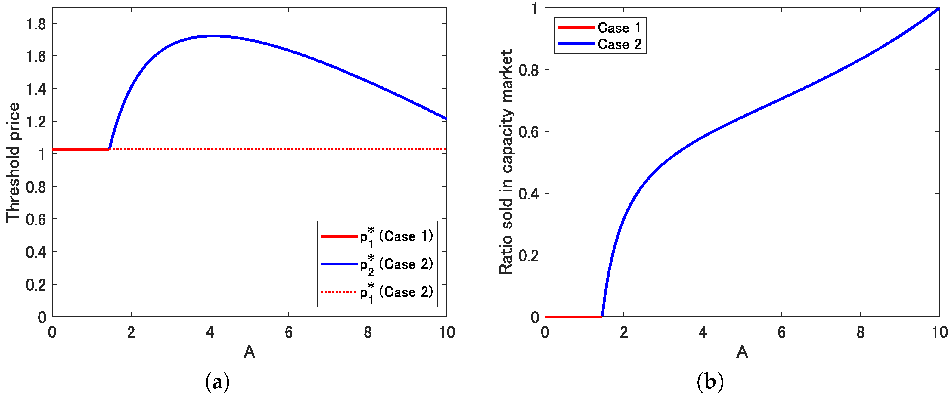
3.2.2. Profit Rate of Capacity Market A

We consider the effect that the profit rate of the capacity market A has on the threshold price p * . Unlike other parameters, p 1 * does not contain A and hence is constant. Concerning p 2 * , we rewrite p 2 * as
p 2 * = β 1 I ( β 1 1 ) θ θ 1 A + 2 B 0 A B 0 2 ,
where θ is defined in (26). p 2 * is the sum of hyperbolic and linear functions of A, each with a negative coefficient since 0 < θ < 1 under condition (13). Then, it is not difficult to check that p 2 * is increasing for 0 < A < A M and decreasing for A M < A < A ¯ , where A M = 1 θ B 0 . This implies that p 2 * is not monotonic in A.
The effects that A has on p 2 * are two-fold. Since the power producer can hedge the price fluctuation risk by selling some amount of capacity in the capacity market, an increase in A will allow the producer to take more risk, and this pushes up p 2 * . As A approaches to A ¯ , immediate investment becomes more attractive since the ratio of the plant sold in the capacity market increases to 1 and the value of waiting comparatively decreases. This pushes down p 2 * . The unimodal shape of p 2 * in terms of A is interpreted as the former effect is dominant for small A, while the latter effect is dominant for larger A. Note also that turning point A M is a decreasing function of all λ , σ 2 , and I. Investment becomes more risky when these parameters increase. Then, p 2 * increases and then decreases for a smaller value of A to avoid risk increase.
When A approaches A ¯ , p 2 * approaches p 2 * ( A ¯ ) = β 1 I ( β 1 1 ) B 0 . It can be checked that p 1 * > p 2 * ( B 0 ) if and only if β 1 > 2 . If this is the case, p 2 * decreases and goes below p 1 * as A approaches A ¯ .
Figure 4 shows a numerical example of p * and 1 K 1 as a function of A. In panel (a), the red solid line is p 1 * , which is constant, and blue solid line is p 2 * . In Case 2, p 2 * increases rather sharply for A 0 = 1.45 < A < A M = 4.08 and gradually decreases for A M < A < A ¯ = 10 . Since β 1 = 1.70 < 2 in this case, we observe that p 2 * ( A ¯ ) > p 1 * . The result indicates that the optimal investment policy depends in the relationship of both prices in electricity and capacity markets. For low capacity price compared to electricity, the investment threshold increases with the profit rate. Intuitively, while the power producers have an incentive to sell the capacity in the market, the investment opportunity decreases because the profit from the electricity market decreases. In contrast, when the profit rate is relatively high, the power producers have a large incentive to invest because enough profit from the capacity market can be obtained. Panel (b) depicts the ratio sold in the capacity market. Similar to Figure 3, the graph starts to increase sharply when A exceeds A 0 , and the slope becomes gentle and approaches 1 as A goes to A ¯ .

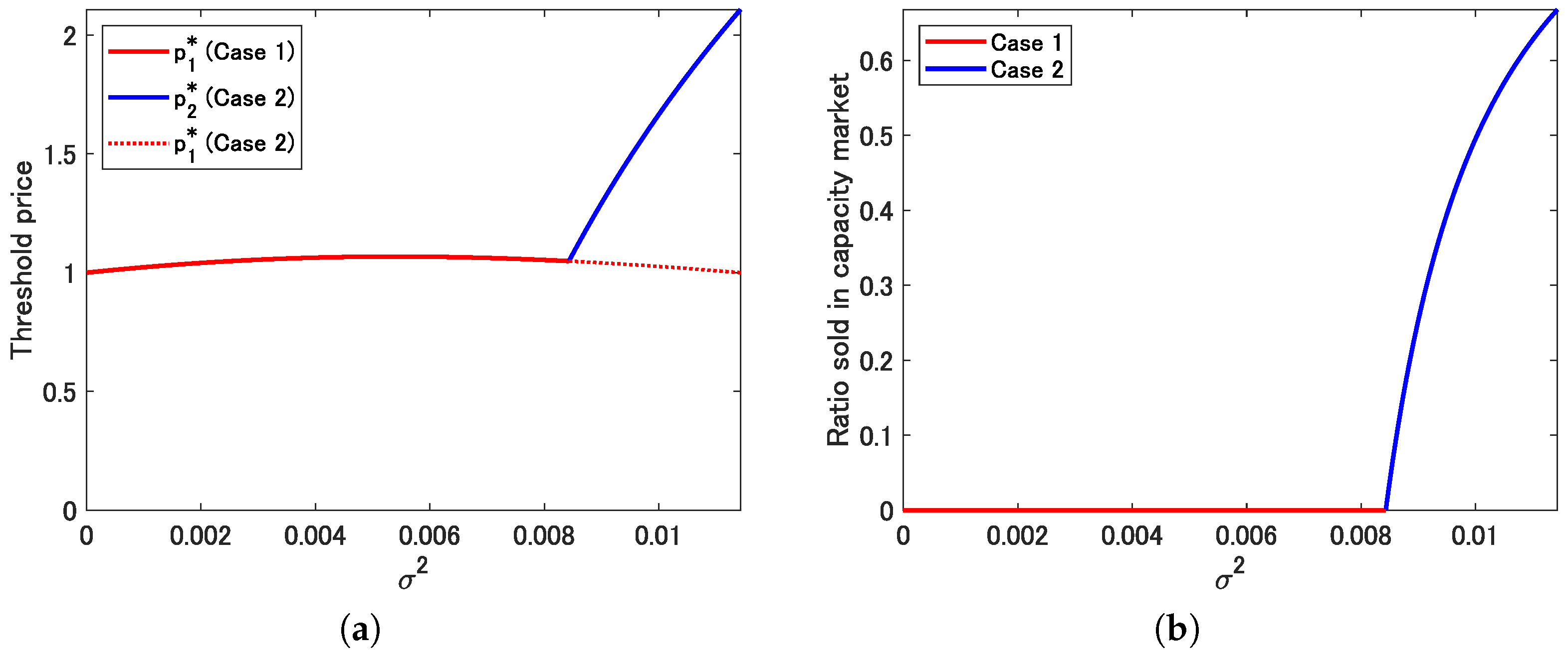
3.2.3. Electricity Price Volatility σ 2

We consider the relation between price volatility σ 2 and the threshold price, as well as the ratio sold in the capacity market. Since not only θ in (22) but also β 1 is dependent on σ 2 , the shape of p 1 * as a function of σ 2 is difficult to analytically derive. Therefore, we investigate it by using a numerical example. Conversely, it is easy to check from (28) that p 2 * increases as σ 2 increases for σ 0 2 = 0.0084 < σ 2 < σ 2 ¯ = 0.0114 .
Panel (a) of Figure 5 shows p * as a function of volatility σ 2 . In this case, p 1 * first increases gradually and then decreases. After switching from p 1 * to p 2 * at σ 0 2 , p 2 * increases rather sharply compared to p 1 * . Panel (b) shows 1 K 1 , which is quite similar to that in Figure 3. The ratio sold in the capacity market increases sharply when σ 2 exceeds σ 0 2 .

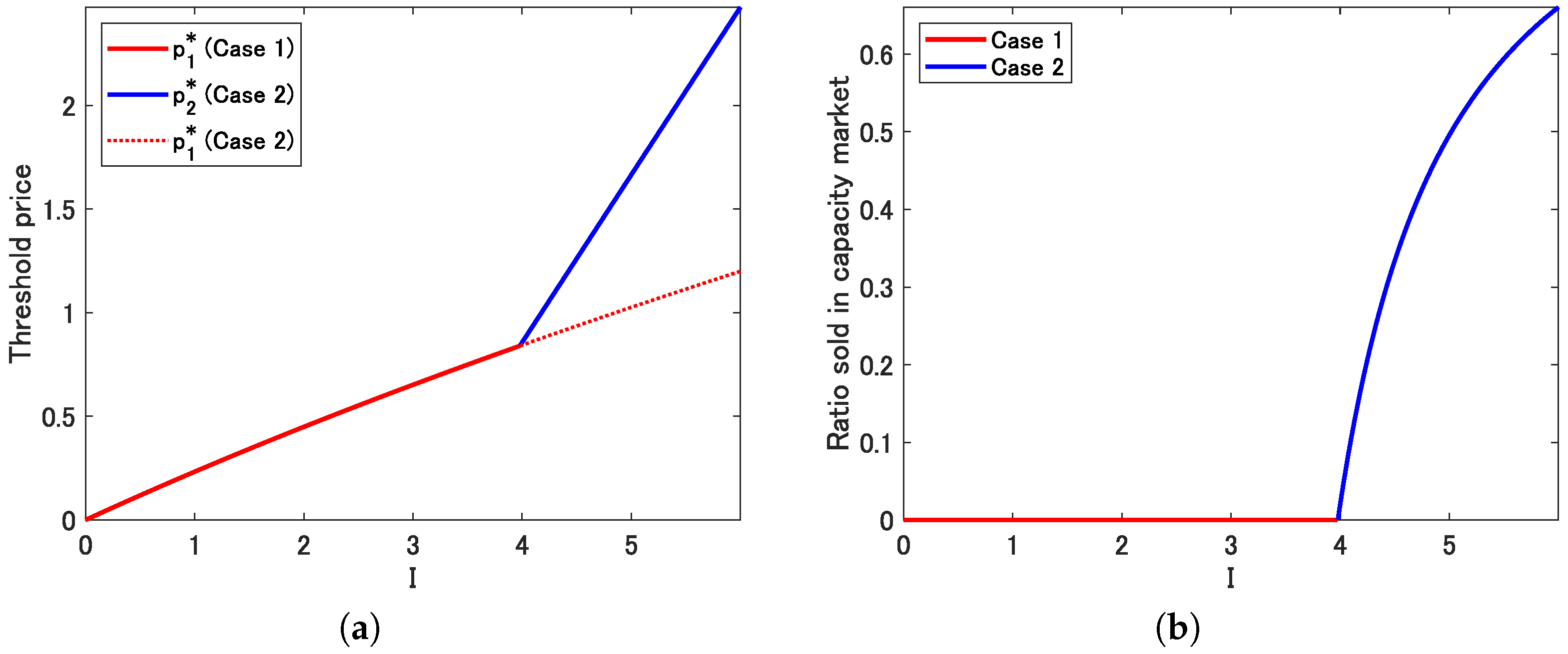
3.2.4. Investment Cost I

Finally, we consider the relation between investment cost I and the threshold price, as well as the ratio of the capacity sold in the capacity market. From (22), it is readily checked that p 1 * is an increasing function of I when β 1 2 . Since p 1 * is rewritten as
p 1 * = η ( D β 1 + 1 ) λ ( 2 β 1 ) ,
we observe that p 1 * is an increasing function even when 1 < β 1 < 2 . Concerning p 2 * , we observe from (28) that p 2 * is a linear function of I with the slope β 1 ( β 1 1 ) A . Thus, threshold price p * always increases as the investment cost increases. If I is large, the power producer will wait until electricity prices go up to a high threshold to cover the high investment cost.
Figure 6 depicts a numerical example. From panel (a), the threshold price switches from p 1 * to p 2 * at I 0 = 3.98 . The slope of increase of p 2 * is steeper than that of p 1 * . We observe from panel (b) that the ratio sold in the capacity market starts to increase sharply when I exceeds threshold I 0 , as observed in Figure 3, Figure 4 and Figure 5.

4. Conclusions

This paper focuses on the interaction between the investment decision for the risk-averse power producer and the policy of the capacity market in the framework of real options. In particular, we show how the risk aversion and the profit rate of the capacity market affect the optimal investment policy. The results indicate that the power producer obtains the selling income in both the electricity and capacity markets when the risk aversion is relatively high, the effect of risk aversion on the investment policy is ambiguous unlike the previous work, and the power producers have a large incentive to invest because enough profit from the capacity market can be obtained when the profit rate of the capacity market is relatively high.
Our study contributes to the argument on the `missing money’ problem, and highlights the relations among the investment opportunity, risk aversion, and the profit rate of the capacity market. If policymakers can observe the risk aversion of power producers, the missing money problem would be resolved by increasing the investment opportunity for the optimal policy of the profit rate of the capacity market. Even if the power producers have less investment opportunities due to low risk aversion, the problem might be mitigated by means of a subsidy policy for the investment cost.
We highlight the importance of understanding the role of the capacity market for the risk-averse power producers that have both problems of investment in power plants and missing money. In this paper, it is assumed that the capacity price is correlated with that of electricity. Since in any realistic case there exists no correlation, it is necessary to mitigate the assumption in the model. Hence, as an extension of our work, the capacity price is modeled as a stochastic process different from the electricity price by estimating the real data for the capacity market. The penetration of power generations from renewable energy sources leads to the missing money problem, and then the capacity market is created due to mitigating the problem. This means that not only local problems such as missing money, but also whole market problems are included. Thus, it also would be important to address social welfare in order to examine an effect of the interaction between the penetration of renewable energy and the capacity market. In addition, the relations between the capacity mechanism and risk aversion for power producers should be investigated by empirical analyses because evidence of the results in this study could be obtained.

Author Contributions

Conceptualization, R.T.; methodology, N.M. and R.T.; software, N.M.; validation, R.T.; formal analysis, N.M.; investigation, R.T.; resources, N.M.; data curation, N.M.; writing—original draft preparation, N.M. and R.T.; writing—review and editing, R.T.; visualization, N.M.; supervision, R.T.; project administration, R.T.; funding acquisition, N.M. and R.T. All authors have read and agreed to the published version of the manuscript.

Funding

This work was supported by JSPS KAKENHI Grant Number JP20H00285.

Institutional Review Board Statement

Not applicable.

Informed Consent Statement

Not applicable.

Data Availability Statement

Not applicable.

Conflicts of Interest

The authors declare no conflict of interest.

Abbreviations

GBMGeometric Brownian motion

Appendix A. Proofs

Appendix A.1. Derivation of (6) and (7)

Let Q t = exp ( μ σ 2 2 ) t + σ W t ) . Then, (6) is obtained from
E P s R P s = p = p E R = p 0 e ρ t E Q t d t = p ρ μ .
Since Q t is a Markov process,
E R 2 = 2 0 t e ρ t e ρ u E Q t Q u d u d t = 2 0 t e ρ t e ρ u E Q t 2 E Q u Q t d u d t = 2 0 t e ρ t e ρ u e ( 2 μ + σ 2 ) t e μ ( u t ) d u d t = 1 ( ρ μ ) ( ρ μ σ 2 2 ) .
From V R = E R 2 E R 2 , (7) is derived from
V P s R P s = p = p 2 V R = p 2 σ 2 2 ( ρ μ ) 2 ( ρ μ σ 2 2 ) .

Appendix A.2. Proof of Theorem 1

Based on [25], we first show the solution of the optimal stopping problem with a general payoff function when the underlying process is a GBM. Let f ( p ) be a function such that f ( p ) > 0 for some p > 0 and E e ρ τ f ( P τ ) P 0 = p is well-defined for every stopping time τ 𝒯 , where P t is a GBM (1). To solve the optimal stopping problem
V ( p ) = sup τ 𝒯 E e ρ τ f ( P τ ) P 0 = p ,
we define
g ( u ) = u β 1 β 1 β 2 f ( u 1 β 2 β 1 )
and let G ( u ) be the smallest non-negative concave majorant of g ( u ) on ( 0 , ) . The following is a simplified version of [25] when P t follows a GBM.
Theorem A1. 
Value function of the optimization problem (A4) is given by
V ( p ) = p β 1 G ( p β 2 β 1 ) , p > 0 .
Proof. 
Since the underlying process is a GBM, we plug ψ ( p ) = p β 1 and ϕ ( p ) = p β 2 into Proposition 5.12 of [25]. The value function is given by V ( p ) = ψ ( p ) W ˜ ( p β 2 β 1 ) for p > 0 where, W ˜ ( y ) is the smallest non-negative concave majorant of H ˜ ( y ) = ( y ) β 1 β 1 β 2 f ( ( y ) 1 β 2 β 1 ) for y < 0 . By replacing y for y < 0 with u > 0 , g ( u ) and G ( u ) correspond to H ˜ ( u ) and W ˜ ( u ) , respectively. □
Theorem A1 reduces an optimal stopping problem to find the smallest non-negative concave majorant G ( u ) . The next result is useful to identify G ( u ) in many applications.
Corollary A1. 
If u * = argmax u > 0 { g ( u ) } exists and lim u g ( u ) u = 0 , then the smallest non-negative concave majorant of g ( u ) is in the form
G ( u ) = G 0 ( u ) , 0 < u u * , g ( u * ) , u > u *
where G 0 ( u ) is the smallest non-negative concave majorant of g ( u ) on ( 0 , u * ] .
Proof. 
It is not difficult to check that G ( u ) in (A7) is a non-negative concave majorant of g ( u ) on ( 0 , ) and is the smallest on ( 0 , u * ] . To prove the minimality on ( u * , ) , suppose that there exists a non-negative concave majorant G ^ ( u ) satisfying G ^ ( u * ) = g ( u * ) and G ^ ( u ^ ) < g ( u * ) for some u ^ > u * . From the concavity of G ^ ( u ) ,
G ^ ( u ) g ( u * ) + G ^ ( u ^ ) g ( u * ) u ^ u * ( u u * ) , u > u ^
which shows lim sup u G ^ ( u ) u G ^ ( u ^ ) g ( u * ) u ^ u * < 0 . Since lim u g ( u ) u = 0 , G ^ ( u ) < g ( u ) holds for sufficiently large u, which contradicts to that G ^ ( u ) is a majorant of g ( u ) . □
We now prove Theorem 1.
Proof of Theorem 1. 
We define
g 1 ( u ) = u β 1 β 1 β 2 f 1 ( u 1 β 2 β 1 ) = γ 2 u β 1 2 β 1 β 2 + B 0 u β 1 1 β 1 β 2 I u β 1 β 1 β 2 .
(Case A) β 1 > 2 : In this case, it is not difficult to check that g 1 ( u ) = 0 has two positive solutions
u ± = ( β 1 1 ± D ) B 0 2 β 1 I β 1 β 2
where D is defined in (24). Similarly, g 1 ( u ) = 0 has two positive solutions
w ± = [ ( β 1 1 ) ( 1 β 2 ) ± D w ] B 0 2 β 1 ( β 2 ) I β 1 β 2
where
D w = ( β 1 1 ) 2 ( 1 β 2 ) 2 β 1 ( β 1 2 ) ( β 2 ) ( 2 β 2 ) θ
that is positive under (13). Moreover, 0 < u < w < u + < w + in this case. Then, we obtain
Energies 16 04241 i001
(Case B) 1 < β 1 2 : In this case, both g 1 ( u ) = 0 and g 1 ( u ) = 0 have unique positive solution u + in (A10) and w + in (A11), respectively. Thus,
Energies 16 04241 i002
attains the maximum at u = u + . Moreover, lim u g 1 ( u ) u = 0 . From Corollary A1, the smallest non-negative concave majorant of g 1 ( u ) is in the form
G 1 ( u ) = G 0 ( u ) , 0 < u < u + , g 1 ( u + ) , u u + .
To obtain G 0 ( u ) , consider a straight line that goes through the origin and is tangent to g 1 ( u ) at some u ( 0 , u + ) . The slope of the straight line connecting ( 0 , 0 ) and ( u , g 1 ( u ) ) is h ( u ) = g 1 ( u ) / u . With some algebra, we can observe that h ( u ) = 0 has two positive solutions:
v ± = ( 1 β 2 ± D ) B 0 2 ( β 2 ) I β 1 β 2
where D is given in (25), and that h ( u ) > 0 for 0 < u < v and u > v + , while h ( u ) < 0 for v < u < v + . This, along with lim u h ( u ) = 0 , imply that slope h ( u ) is the maximum at u = v . Moreover, v < u + since g 1 ( v ) > 0 , and v > w in Case A since g 1 ( v ) < 0 . Then, the smallest non-negative majorant for 0 < u < u + is given by
G 0 ( u ) = g 1 ( v ) u , 0 < u v , g 1 ( u ) , v < u < u + .
The value function is now derived from Theorem A1 by noting that p 1 * = ( u + ) 1 β 2 β 1 and p 1 = ( v ) 1 β 2 β 1 . □

Appendix A.3. Proof of Theorem 2

As in the proof of Theorem 1, we define
g 2 ( u ) = g c ( u ) , 0 < u < u 0 , g 1 ( u ) , u u 0
where u 0 = p 0 β 2 β 1 , g 1 ( u ) is defined in (A9) and
g c ( u ) = u β 1 β 1 β 2 f c ( u 1 β 2 β 1 ) = ( β 1 1 ) A β 1 β 1 β 1 1 u β 1 1 β 1 β 2 p 2 * u β 1 β 1 β 2 .
Here, the second equality follows from (28). It is noted that g 1 ( u ) < g c ( u ) for 0 < u < u 0 since f 1 ( p ) < f c ( p ) for p > p 0 . Further, g 1 ( u ) and g c ( u ) are smoothly pasted at u = u 0 ; that is g 1 ( u 0 ) = g c ( u 0 ) and g 1 ( u 0 ) = g c ( u 0 ) .
From
g c ( u ) = ( β 1 1 ) A β 1 β 2 u β 2 β 1 β 2 u 1 β 1 β 2 p 2 * ,
g c ( u ) = ( β 1 1 ) ( 1 β 2 ) A ( β 1 β 2 ) 2 u 2 β 2 β 1 β 1 β 2 u 1 β 1 β 2 ( β 2 ) 1 β 2 p 2 * ,
g c ( u ) is increasing and concave for u > 0 if p 2 * 0 . If p 2 * > 0 , the shape of g c ( u ) is given as
Energies 16 04241 i003
where
x 1 = ( p 2 * ) β 2 β 1 ,
x 2 = ( β 2 ) 1 β 2 p 2 * β 2 β 1 .
(Case 1) p 2 * p 0 : Since p 2 * p 0 is equivalent to u 0 < x 1 , g c ( u 0 ) = g 1 ( u 0 ) > 0 , which in turn implies u 0 < u + from (A13) and (A14). Thus, g 2 ( u ) attains the maximum at u = u + . From Corollary A1, the smallest non-negative majorant of g 2 ( u ) is
G 2 ( u ) = g c ( u ) , 0 < u u 0 , g 1 ( u ) , u 0 < u u + , g 1 ( u + ) , u > u + .
The concavity of G 2 ( u ) can be checked from the concavity of g c ( u ) , (A13) and (A14), and the smooth pasting conditions. V 2 ( p ) in (29) is obtained from Theorem A1.
(Case 2) p 2 * > p 0 : Since u 0 > x 1 in this case, g c ( u 0 ) = g 1 ( u 0 ) 0 , and thus u 0 u + from (A13) and (A14). The maximum of g 2 ( u ) is given by u = x 1 . Since g 2 ( u ) is concave for 0 < u < x 1 , the smallest non-negative majorant is obtained from Corollary A1 as
G 2 ( u ) = g c ( u ) , 0 < u x 1 , g c ( x 1 ) u > x 1 .
Theorem A1 now proves V 2 ( p ) in (30). □

Appendix A.4. Proof of Theorem 3

Noting that K can be rewritten as
K = β 1 2 ( β 1 1 ) θ 1 A / B 0 1 θ A / B 0 + 1 ,
clear K / x > 0 for x { λ , A , I } . For x { λ , I } , θ 0 when x 0 and θ 1 when x x ¯ . From 0 < A < B 0 , we observe that lim x 0 K < 0 , and lim x x ¯ K > 1 , which proves the desired result for x { λ , I } . Case x = A is also easy to show since lim A 0 K = and lim A A ¯ K = .
The remaining case is x = σ 2 . From (28), K > 0 if and only if σ 2 > σ m 2 , where σ m 2 = ( ρ μ ) λ I ( 1 A / B 0 ) 2 + 1 2 1 . For σ 2 > σ m 2 , K / σ 2 > 0 since, as σ 2 increases, θ increases, while β 1 decreases. Noting that θ 1 as σ 2 σ 2 ¯ , lim σ 2 σ 2 ¯ K > 1 as before. This completes the proof for σ 2 . □

References

  1. Joskow, P.L. Capacity payments in imperfect electricity markets: Need and design. Util. Policy 2008, 163, 159–170. [Google Scholar] [CrossRef]
  2. Green, R.; Staffell, I. Electricity in Europe: Exiting fossil fuels? Oxf. Rev. Econ. Policy 2016, 32, 282–303. [Google Scholar] [CrossRef]
  3. Woo, C.K.; Ho, T.; Zarnikau, J.; Olson, A.; Jones, R.; Chait, M.; Horowitz, I.; Wang, J. Electricity-market price and nuclear power plant shutdown: Evidence from California. Energy Policy 2014, 73, 234–244. [Google Scholar] [CrossRef]
  4. Newbery, D. Missing money and missing markets: Reliability, capacity auctions and interconnectors. Energy Policy 2016, 94, 401–410. [Google Scholar] [CrossRef]
  5. Bublitz, A.; Keles, D.; Zimmermann, F.; Fraunholz, C.; Fichtner, W. A survey on electricity market design: Insights from theory and real-world implementations of capacity remuneration mechanisms. Energy Econ. 2019, 80, 1059–1078. [Google Scholar] [CrossRef]
  6. Duggan, J.E., Jr. Capacity market mechanism analyses: A literature review. Curr. Sustain. Energy Rep. 2020, 7, 186–192. [Google Scholar] [CrossRef]
  7. De Vries, L.; Heijnen, P. The impact of electricity market design upon investment under uncertainty: The effectiveness of capacity mechanisms. Util. Policy 2008, 16, 215–227. [Google Scholar] [CrossRef]
  8. Hach, D.; Spinler, S. Capacity payment impact on gas-fired generation investments under rising renewable feed-in—A real options analysis. Energy Econ. 2016, 53, 270–280. [Google Scholar] [CrossRef]
  9. Höschle, H.; De Jonghea, C.; Le Cadre, H.; Belmans, R. Electricity markets for energy, flexibility and availability—Impact of capacity mechanisms on the remuneration of generation technologies. Energy Econ. 2017, 66, 372–383. [Google Scholar] [CrossRef]
  10. Hach, D.; Spinler, S. Robustness of capacity markets: A stochastic dynamic capacity investment model. OR Spectr. 2018, 40, 517–540. [Google Scholar] [CrossRef]
  11. Rios-Festner, D.; Blanco, G.; Olsina, F. Long-term assessment of power capacity incentives by modeling generation investment dynamics under irreversibility and uncertainty. Energy Policy 2020, 137, 111185. [Google Scholar] [CrossRef]
  12. de Maere d’Aertryckea, G.; Ehrenmanna, A.; Smeers, Y. Investment with incomplete markets for risk: The need for long-term contracts. Energy Policy 2017, 105, 571–583. [Google Scholar] [CrossRef]
  13. Petitet, M.; Finon, D.; Janssen, T. Capacity adequacy in power markets facing energy transition: A comparisonof scarcity pricing and capacity mechanism. Energy Policy 2017, 103, 30–46. [Google Scholar] [CrossRef]
  14. Ousman, A.A.; Hary, N.; Rious, V.; Saguan, M. The impact of investors’ risk aversion on the performances of capacity remuneration mechanisms. Energy Policy 2018, 112, 84–97. [Google Scholar] [CrossRef]
  15. Basak, S.; Chabakauri, G. Dynamic mean-variance asset allocation. Rev. Financ. Stud. 2010, 23, 2970–3016. [Google Scholar] [CrossRef]
  16. Dixit, A.K.; Pindyck, R.S. Investment under Uncertainty; Princeton University Press: Princeton, NJ, USA, 1994. [Google Scholar]
  17. Hugonnier, J.; Morellec, E. Real options and risk aversion. In Real Options, Ambiguity, Risk and Insurance; Bensoussan, A., Peng, S., Sung, J., Eds.; IOS Press: Amsterdam, The Netherlands, 2013; pp. 52–65. [Google Scholar]
  18. McDonald, R.L.; Siegel, D.S. The value of waiting to invest. Q. J. Econ. 1986, 101, 707–728. [Google Scholar] [CrossRef]
  19. Chronopoulos, M.; De Reyck, B.; Siddiqui, A. Optimal investment under operational flexibility, risk aversion, and uncertainty. Eur. J. Oper. Res. 2011, 213, 221–237. [Google Scholar] [CrossRef]
  20. Chronopoulos, M.; Lumbreras, S. Optimal regime switching under risk aversion and uncertainty. Eur. J. Oper. Res. 2017, 256, 543–555. [Google Scholar] [CrossRef]
  21. Barbosa, L.; Ferrão, P.; Rodrigues, A.; Sardinha, A. Feed-in tariffs with minimum price guarantees and regulatory uncertainty. Energy Econ. 2018, 72, 517–541. [Google Scholar] [CrossRef]
  22. Detemple, J.; Kitapbayev, Y. The value of green energy under regulation uncertainty. Energy Econ. 2017, 89, 104807. [Google Scholar] [CrossRef]
  23. Babich, V.; Lobel, R.; Yücel, S. Promoting solar panel investments: Feed-in-tariff vs. tax- rebate policies. Manuf. Serv. Oper. Manag. 2021, 22, 1148–1164. [Google Scholar] [CrossRef]
  24. Conejo, A.J.; Carrión, M.; Morales, J.M. Decision Making under Uncertainty in Electricity Markets; Springer: New York, NY, USA, 2010. [Google Scholar]
  25. Dayanik, S.; Karatzas, I. On the optimal stopping problem for one-dimensional diffusions. Stoch. Process. Their Appl. 2003, 107, 173–212. [Google Scholar] [CrossRef]
Figure 1. Flowchart of the model analysis.
Energies 16 04241 g001
Figure 2. (a) Value function V 2 ( p ) in Case 1. (b) Value function V 2 ( p ) in Case 2. Note: Red solid line represents V 2 ( p ) . For comparison, f 1 ( p ) , p 1 * , and p 0 are plotted in (a), and f 1 ( p ) , f c ( p ) , p 0 , and p 2 * are plotted in (b). In (a), μ = 0.02 , ρ = 0.04 , σ 2 = 0.01 , λ = 0.15 , A = 3 , B 0 = 10 , and I = 5 . In (b), λ = 0.25 and other parameters are the same as in (a).
Energies 16 04241 g002
Figure 3. (a) Threshold price and risk aversion coefficient λ . (b) Ratio sold in the capacity market and risk aversion coefficient λ . Note: Red and blue solid lines represent Cases 1 and 2, respectively. For comparison, p 1 * in Case 2 is plotted by a red dashed line in (a). μ = 0.02 , ρ = 0.04 , σ 2 = 0.01 , A = 3 , B 0 = 10 , and I = 5 .
Energies 16 04241 g003
Figure 4. (a) Threshold price and profit rate of capacity market A. (b) Ratio sold in the capacity market and profit rate of capacity market A. Note: Red solid line shows Case 1 and blue solid line shows Case 2. For comparison, p 1 * in Case 2 is plotted by a red dashed line in (a). μ = 0.02 , ρ = 0.04 , σ 2 = 0.01 , I = 5 , B 0 = 10 , λ = 0.25 .
Energies 16 04241 g004
Figure 5. (a) Threshold price and price volatility σ 2 . (b) Ratio sold in the capacity market and price volatility σ 2 . Note: Red and blue solid lines represent Cases 1 and 2, respectively. For comparison, p 1 * in Case 2 is plotted by a red dashed line in (a). μ = 0.02 , ρ = 0.04 , I = 5 , A = 3 , B 0 = 10 , and λ = 0.25 .
Energies 16 04241 g005
Figure 6. (a) Threshold price and investment cost I. (b) Ratio sold in the capacity market and investment cost I. Note: Red and blue solid lines represent Cases 1 and 2, respectively. For comparison, p 1 * in Case 2 is plotted by a red dashed line in (a). μ = 0.02 , ρ = 0.04 , σ 2 = 0.01 , A = 3 , B 0 = 10 , and λ = 0.25 .
Energies 16 04241 g006
Disclaimer/Publisher’s Note: The statements, opinions and data contained in all publications are solely those of the individual author(s) and contributor(s) and not of MDPI and/or the editor(s). MDPI and/or the editor(s) disclaim responsibility for any injury to people or property resulting from any ideas, methods, instructions or products referred to in the content.

