Abstract
Transformer excitation magnetizing curves (TEMC) reflect the dynamic operation characteristics of iron-core materials. Using numerical analysis and the waveform recording function of digital oscilloscopes, we developed a cost-effective method for determining the TEMC. This approach eliminates the need for conventional analog integrator circuits. To address the potential obstacles to the digital generation of TEMC—namely, curve offsets and curve transients—we proposed solutions involving Fourier filtering and determining the initial point of integration. The results indicate that the proposed approach yields results consistent with those of conventional analog integrator circuits and highlight its promise for applications in data processing.
1. Introduction
Transformer excitation magnetizing curves (TEMC) reflect dynamic responses, such as harmonics, inrush current, and losses, and hysteresis characteristics are typically measured using silicon steel sheets [1]. However, because of the potential formation of an extremely thin insulating layer between lamination steels and the formation of gaps between stacked and stamped lamination steels, whether the characteristics of a single material are retained after assembly remains unknown [2]. These factors may affect the characteristics of magnetic circuits. Generally, TEMC reflects the relationship between the magnetizing force (H) and magnetic flux density (B), also called the B–H curve. Because of magnetic saturation and magnetic hysteresis, this curve is a closed loop.
Epstein frames, composed of four symmetrical iron cores wound around two sets of coils, are used to assess hysteresis characteristics [3]. Another common method of evaluating hysteresis characteristics is to use a magnetic yoke with a Hall sensor and a pick-up coil [4,5,6]; before the B–H curve is calculated, the magnetic flux density is determined through the integration of the voltage signal of the induction coil. The conventional approach is to use an analog integrator that includes integrating circuits composed of capacitor and resistor components [1,7] and integrators composed of active components [8]. However, with the popularization of data-capturing cards, digital integrator circuits are expected to be used in the future [9,10,11].
To digitally integrate a voltage signal and accurately determine magnetic flux density, noise and DC components must be considered [12]. Pólik and Kuczmann [7] used the fast Fourier transform for noise filtering. Because commercial electric sources may have harmonic components, whether the source used in tests exhibits harmonics should be considered. Chatterjee et al. [8] analyzed the effects of several power supply harmonics and suggested that, with increased source harmonics, transformers can be operated below the rated voltage to reduce the winding current and prolong service life. Some studies have also proposed digital methods for deriving B–H curves and highlighted the lack of discussion regarding problems that may lead to incorrect B calculation [13,14,15,16]. Notice that the methods of literature are based on four sets of silicon steel sheets that are not suitable for a transformer. In addition, the test voltage source of the literature is a pure sinusoidal waveform that is not feasible to test a power transformer. Hence, the frequency and harmonics can be problematic if the test source is applied from the electric grid. Herein, we present proposed solutions for the aforementioned problems as well as the experimental results of testing our solutions.
The rest of this paper is organized as follows. Section 2 explains the specifications of the test object and the calculation of the magnetization curve. Section 3 discusses how the magnetization curve of the test object was obtained using the conventional circuit integration method. Section 4 introduces a digital method for deriving B–H curves and discusses the validation of this method based on an ideal power supply and one featuring harmonics.
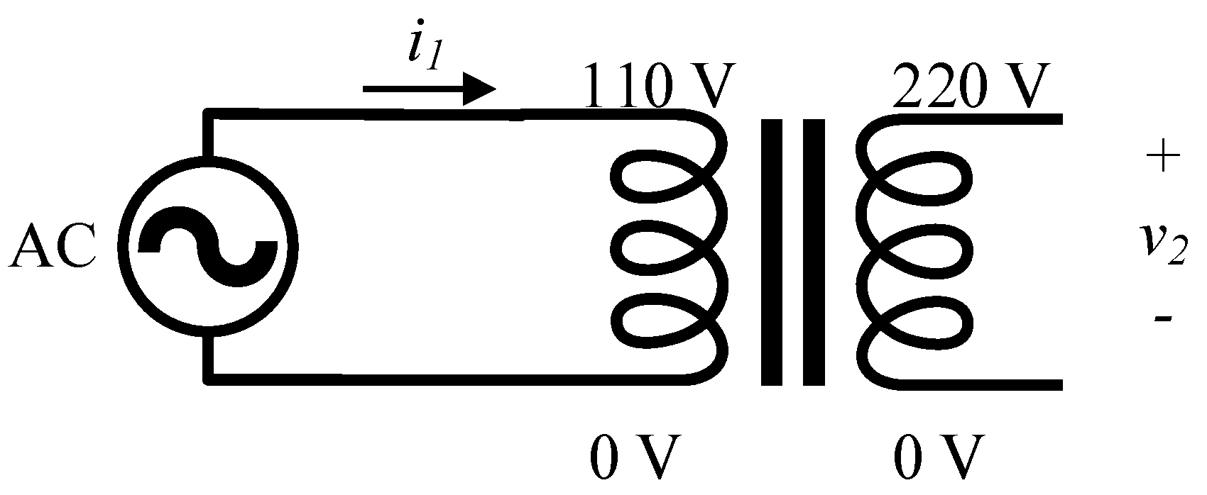
2. Transformer Specifications and Measurements
In this study, the specified capacity of the transformers used was a single-phase 500 VA, and the nominal voltages of the low-voltage and high-voltage sides were 110 and 220 V, respectively, with a rated frequency of 60 Hz. As shown in Figure 1, the iron core was shell-type and made of lamination steel. The dimensions of the iron core are listed in Table 1. The length of the equivalent magnetic path () and the equivalent cross-sectional area () were calculated using Equations (1) and (2) [12]. After the core size was recorded (Table 1).
Figure 1.
Transformer core.
Table 1.
Parameters of the tested transformer.
The magnetic field strength and the magnetic flux density will be simplified to Equations (3) and (4), respectively, because of the no-load situation. The magnetic field strength H is the product of the primary current of the transformer and , and the magnetic flux density B is the product of the voltage of the secondary side of the transformer and after integration.
where is the excitation current from the primary winding (A) and is the secondary voltage (V).
From the transformer parameters listed in Table 1, and were derived. The calculated B and H values were then plotted on the x-axis for the primary-side current waveform. After the primary voltage waveform was integrated and converted into y values, the magnetization (B–H) curve, i.e., TEMC was plotted.
In the simulation of an electrical circuit, the B–H curve can be replaced by the flux (V.s) and the magnetization current (A) because the equivalent flux path length and the equivalent core cross-sectional area are not easy to calculate accurately.
3. Signal Processing of Analog-Circuit B–H Curves
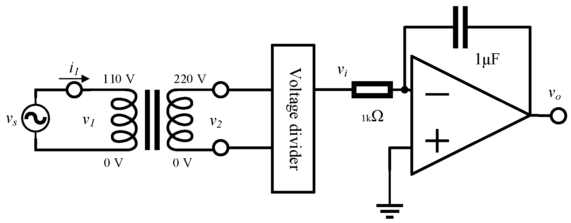
Active Integrator Circuit
As shown in Figure 2, a common inverting integrator circuit was used to integrate the voltage on the secondary side of the voltmeter. A voltage divider attenuated the input signal to match the input range of the inverting integrator, that is, the voltage range of the working power supply. The input voltage of the integrator was fixed to allow the amplifier to operate in the linear region.
Figure 2.
Diagram of the circuit for measuring transformer current and integrating voltage.
As indicated by Equation (7), the input of the inverting integrator circuit was a sinusoidal signal (V) with a magnitude , angle frequency , and phase angle starting at the maximum voltage. The output signal was calculated using Equation (8) and the phasor of the output signal was calculated using Equation (9).
The inverting integrator circuit included peripheral components, such as a resistor (1 kΩ) and a capacitor (1 μF). Through the insertion of the parameters into Equations (8) and (9), the peak ratio of the output to the input signal was derived as , with a phase angle of .
When a Vrms of 110 V was applied to the primary side of the transformer, the secondary-side voltage became 220 V (Vrms). To avoid exceeding the operating voltage of the operational amplifier (±15 V) and prevent waveform distortion, a passive probe with an attenuation ratio of 200:1 was used to measure the secondary voltage of the transformer. After attenuation by the passive probe, the signal was determined to be a range of ±1.56 (V), meeting the aforementioned requirements. In Equation (4), the is replaced by 200 times of and the equals zero for pre-demagnetizing; thus, the flux density is given by:
A DSOX3014T oscilloscope (Keysight) with four channels, a bandwidth of 100 MHz, a sampling rate of 1 GS/s, and a memory depth of 4 MB was used. The voltage source used was an APS-7100 AC power supply (GWInstek).
The oscilloscope revealed the input and output voltage signals of the integrator. Figure 3 shows the attenuated voltage of the transformer’s secondary-side , the transformer’s primary-side current i1, the integrator output, and the transformer’s primary-side voltage. The AC coupling function of the oscilloscope removes not only the DC offset but also some low-frequency signals; thus, this function was not used to avoid distortion.
Figure 3.
Integrator waveform diagram, where ch1 (yellow) is the attenuated voltage of the transformer’s secondary-side, ch2 (green) is the transformer’s primary-side current, ch3 (blue) is the integrator output, and ch4 (red) is the transformer’s primary-side voltage.
As shown in Figure 4a, the output signal of the integrator (integrated voltage) was reversed from that of the oscilloscope setting because of the polarity inversion of the integrator. The two signals of the primary current and integration of secondary voltage had a minor DC offset, which may have affected the B–H plot.
Figure 4.
B–H curve plotted by oscilloscope. (a) Primary current (yellow) and integration of secondary voltage (green, reversed from the oscilloscope setting) (b) B–H curve (without calibration) plotted from (a).
As shown in Figure 4b, when the oscilloscope’s XY mode (Lissajous pattern) was used, an equal-ratio B–H curve was obtained. Specifically, the x- and y-axes were set as the current of the primary side and the output voltage of the integrating circuit, respectively. Additionally, the channel of the output voltage of the integrating circuit was inverted to have the same polarity as that of the input signal. The oscilloscope cannot be used to multiply the primary-side current and the output voltage of the integrator circuit by and as in Equations (3) and (4). Therefore, these coefficients were used only as references for relevant comparisons. As indicated by the DC offset, both the x- and y-axes shifted on the B–H curve.
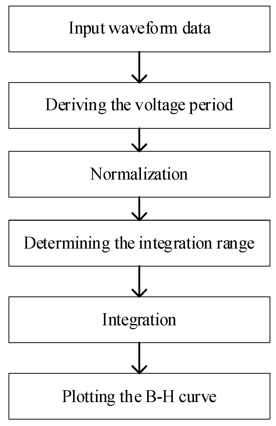
4. Digital B–H Signal Processing
The proposed approach in this study involves digital processing and analysis. The test requires only an oscilloscope that can store waveforms processed through computerized numerical analysis. This approach helps to avoid the aforementioned phase shift problem of analog circuits and is cost-effective.
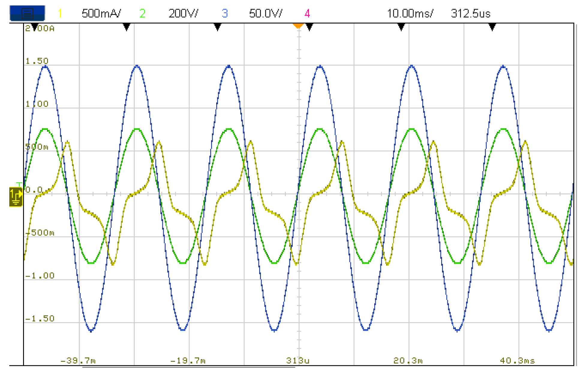
4.1. Test Structure and Settings
The oscilloscope and voltage source used to test this method were identical to those described earlier; the test structure is presented in Figure 5. A voltage of 110 V and a frequency of 60 Hz were applied to the low-voltage side of the transformer. Subsequently, the current i1 on the low-voltage side of the transformer and the voltage v2 on the high-voltage side of the transformer were measured using the oscilloscope. The built-in high-frequency noise-filtering function can be turned on or off optionally; the average capture mode was selected to reduce noise interference. Special care was taken to ensure that the oscilloscope channel for AC coupling was not selected.
Figure 5.
Circuit diagram without an integrator.
A screenshot from the oscilloscope is shown in Figure 6. The current of the low-voltage side i1 is illustrated as Channel 1 (yellow), the voltage of the high-voltage side v2 is illustrated as Channel 2 (green), and the low-voltage side is illustrated as Channel 3 (blue). The voltages on the primary and secondary sides of the transformer were 109.49 and 220.54 V, respectively, which accord with the nominal voltage of the equipment. The no-load current on the primary side was 365.83 mA, and the no-load loss was calculated as 40.05 W.
Figure 6.
Circuit diagram without an integrator, in which ch1 (yellow) is the current on the low-voltage side of the transformer, ch2 (green) is the voltage on the high-voltage of the transformer, and ch3 (blue) is the voltage on the low-voltage of the transformer.
Because data are processed by numeric analysis, waveforms of more than two cycles should be displayed on the screen. If the data have few observation periods can affect subsequent Fourier transformations and result in poor frequency resolution; however, too many observation periods can reduce the temporal resolution of the data for a given storage capacity. Additionally, if the oscilloscope data are stored as a CSV file, this file should be converted into an XLS file to facilitate subsequent use.
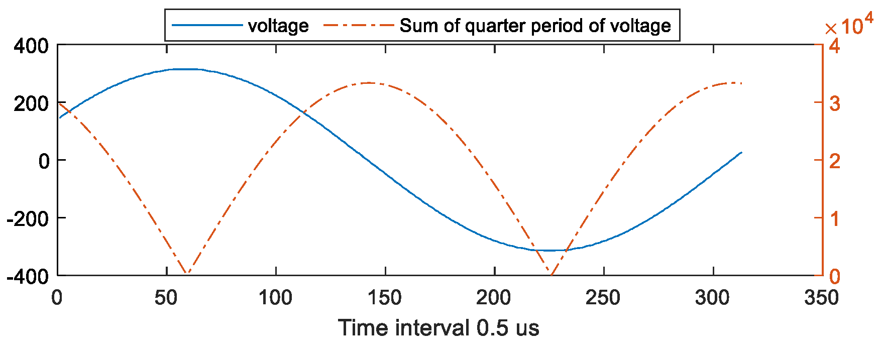
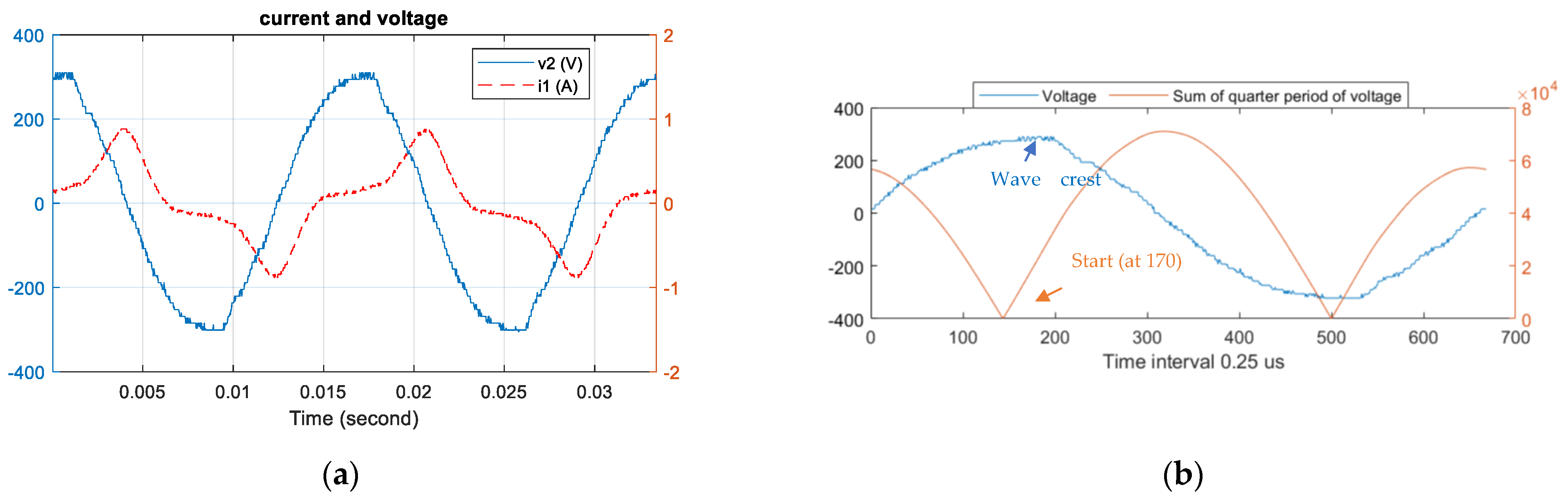
4.2. Method of Calculating Magnetic Flux Density
4.2.1. Effects of Initial Integration Position and Voltage Phase
As indicated by Equation (4), the magnetic flux density B waveform can be derived through the integration of the voltage waveform. However, the voltage phase at the initial time of integration determines the presence of a DC component. If corresponds to a wave crest (positive or negative), the waveform becomes the flux density B waveform after integration. Otherwise, a DC component is present, which is particularly pronounced when the voltage phase is at is zero.
Figure 7a depicts voltage integration starting at a voltage of zero (0°). The voltage integration is from 0 to 1.5 (Vs), which is equivalent to the height of a waveform shifted upward by the height of one wave crest. Conversely, if the voltage integration process started at 180° within the voltage phase, then the integration waveform would shift downward by the height of one wave crest. To eliminate DC components, the initial integration position must be at the crest point of voltage, which is 90° or 270°.
Figure 7.
Effect on the B–H curve of the initial integration position of the voltage phase at 0°. (a) The voltage integration waveform shifted upward. (b) B–H curve shifted upward.
As indicated in Figure 7b, the aforementioned offset of the voltage integration waveform further shifted the B–H curve upward along the B-axis, and the flux density B became distributed between 0 and 2.7 T. However, these plots are incorrect and do not reflect the actual situation.
4.2.2. Effects of DC Components
Although power transformers employ ac, they may be affected by measuring equipment and the surrounding environment, and a measurement signal may include common-mode signals, such as those of DC components. Figure 8a shows voltage integration starting at 0°, and the voltage signal included DC components, with an upward-shifted positive wave crest of 304 V and a negative wave crest of −324 V, indicating a DC offset of −10 V.
Figure 8.
Effects of DC components of a voltage signal. (a) Voltage integration shifting downward with time. (b) B–H curve with multiple loops.
After the DC component of the voltage signal was integrated, the effect observed was expected to increase or decrease over time. Figure 8b shows the B–H curve, in which the voltage integration waveform gradually shifts downward with time, resulting in an incoherent distribution of three loops in the B–H curve.
4.3. Proposed Magnetization Curve Calculation Method
To investigate the aforementioned problems and proposed solutions, we used MATLAB for data processing. Figure 9 depicts a flowchart of data processing steps, which consist of reading the data, removing the DC offset, deriving the voltage period, determining the initial integration points, performing the integration, and plotting the B–H curve. These steps are described in the following sections:
Figure 9.
Flowchart of digital integration.
Step 1: Input waveform data
The data captured by the oscilloscope are input into MATLAB using the “readmatrix” command. The signal acquisition frequency is included. Otherwise, the recording time can be used to derive the frequency.
Step 2: Deriving the voltage period
Because the proposed method utilized a voltage source from an electric grid, the actual voltage frequency changes with time, it should not be a nominal value (60 Hz). The general requirement is to keep fluctuations within ±0.05 Hz.
The voltage period can be derived using Fourier transform. Because the fundamental frequency dominates the voltage signal, the inverse of the frequency corresponding to the maximum signal is the period. Given that the voltage signal in this study was determined to have a dominant frequency of 60.06 Hz and a period of 16.65 ms, the errors between the actual frequency and the period were 0.06 Hz and 0.0167 ms, respectively, compared with the nominal values.
Step 3: Normalization
In this step, the cycle length derived in the previous step is used to calculate an integer multiple of the desired observed length. For example, for a data length of 333 for one period, a period of 666 or another multiple can be selected.
If the length of the acquired data is not an integer multiple of the observed signal period, then the subsequent processing is adversely affected. For example, the average value of a sinusoidal signal should be zero. However, if the calculated length is 3/2 cycles, then the average value is 0.2121, which cannot be regarded as a DC offset. However, the same problem can be encountered in Fourier analysis.
The data lengths for the positive and negative polarities should be the same. A considerable difference implies the presence of a DC component, and the mean value can be subtracted. Errors still occur if only the mean value is subtracted before the complete period length is derived.
Step 4: Determining the integration range
As indicated earlier, when a sinusoidal signal is integrated from an initial point at 90° or 270° in phase, then the integration waveform is a falling sinusoidal signal at 90°, and the DC component is zero. However, in real-life scenarios, the voltage signal may contain noise and harmonics, and the signal may have a nonuniform shape. In addition, the recorded waveform may start at any voltage phase. Therefore, determining the position of the wave crest is challenging. If the voltage signal is a pure sine wave, then the crest is at 90°, which can be confirmed using a wave crest detection approach. However, when the voltage signal has harmonic components, the 90° phase may not be the peak; thus, integration generates an offset.
We propose an equal-area method for deriving the initial integration value, and we use a half cycle as the search frame. Our principle is that if the initial value of the integration waveform must be zero, then the positive and negative half cycles must be included in the integration range to cancel each other out. When the search frame scans the voltage waveform, the process is similar to the concept of using moving windows. When the starting point of the frame moves to the peak voltage value, the sum of the waveform values in the frame becomes zero.
Step 5: Integration
Our method uses a simple FOR loop for voltage integration. We leveraged the following pseudocode, where v is the voltage, A represents the integrated value of voltage, and n is the data number:
for n = 2–data length
end
Step 6: Plotting the B–H curve
By substituting the value of the primary magnetization current i1 into Equation (3), the derived magnetic field strength H can be taken as the x value. Similarly, by substituting the secondary voltage v2 into Equation (4), the derived magnetic flux density B can be taken as the y value.
4.4. Test Results
The dominant frequency calculated from the analysis of the voltage waveform in Figure 7 (Step 2) was 60 Hz, which accorded with the nominal specifications of the power supply. Figure 10 shows the value derived in Step 4 from the voltage waveform through a half-cycle frame (represented by a dotted line). The position corresponding to the lowest point of the sum was the peak of voltage and the initial position of integration.
Figure 10.
Using the sum of the quarter to find the initial integration position of pure sine wave.
Figure 11a shows the voltage integration process (Step 5) starting at 90° within the voltage phase. The DC components were filtered out through subtraction of the mean value. Thus, the two aforementioned integration problems did not occur. Figure 11b shows that the B–H curve (plotted in Step 6) was symmetrical in both the x- and y-directions, which resulted from the factoring out of data-processing errors.
Figure 11.
Integration waveform and B–H curve after correcting initial integration position and removing the DC components. (a) Normal voltage integration waveform. (b) Normal B–H curve.
4.5. Effects of Harmonics on Measurements
The digital method of magnetic characterization tool utilized a pure sinusoidal waveform as a test source, but it might not be capable of testing a power transformer [3]. A practical solution is using a voltage source from the electric grid. However, the frequency and harmonic will cause error measurements.
As mentioned earlier, the wave crest of a purely sinusoidal voltage waveform should be located at 90° in phase. However, in real-life scenarios, the power supply often has harmonic content. Thus, the crest is not usually at 90°, which can result in integration errors. Figure 12a shows the transformer’s primary-side current and secondary-side voltage during an open-circuit test with a distorted voltage source. The secondary-side voltage wave crest was not at 90°. As shown in Figure 12b, the wave crest was at point 191; each cycle contained 667 points equivalent to 103° in the voltage phase. The minimum value obtained through the equal-area method proposed in this study was at point 170, equivalent to 91° in the voltage phase.
Figure 12.
Integration waveform after correction of initial position and removal of DC components. (a) Distorted voltage integration waveform (b) Using the sum of the quarter to find the initial integration position of the harmonics-based sine wave.
Figure 13a presents the voltage integration starting at 103° in the voltage phase (wave crest), indicating an offset of approximately 0.1 T in the B-axis direction. Figure 13b shows the voltage integration process starting at 91°, indicating no offset error in the B-axis direction. The figure also shows the correct characteristics of the magnetization curve.
Figure 13.
B–H curves from a test using a voltage source with harmonic content. (a) B offset error (b) After correction of initial integration position and removal of the DC components.
5. Conclusions
The hysteresis characteristics of transformers are conventionally represented by using silicon steel sheets. However, the factors of assembly and coils are neglected and may affect the characteristics of magnetic circuits. In addition, the digital method in a good deal of the literature might not be suitable for a power transformer. A practical solution is using voltage sources from the electric grid. However, some issues will cause error measurements.
In this study, the proposed method is suitable for power transformers and can against the variation of frequency and harmonic effects. This paper describes two cases with the potential for incorrect B calculation: one case involving a voltage signal containing a DC component, which can lead to a transient response during integration, and another case involving B error resulting from an initial point of integration that is not at 90° of the voltage phase.
Given the aforementioned potential calculation errors, we first derived the complete cycle of signals and then used an equal area to determine the initial phase. In addition to tests using a purely sinusoidal power supply, tests using a voltage source with harmonic content were conducted. The results indicated that the proposed method can be used to derive B–H curves, with or without harmonics. In the simulation of an electrical circuit, the B–H curve can be replaced by the flux (V.s) and the magnetization current (A) that are also available by the proposed method.
Because the proposed method requires only a digital oscilloscope, it is convenient for on-site measurements and in-class experiments. The only challenge lies in the need for integration and Fourier transform in data processing, but these can be performed on a common personal computer.
Author Contributions
Conceptualization, methodology, software, validation, formal analysis, investigation, resources, data curation, and writing—original draft preparation, C.-H.C.; writing—review and editing, supervision, C.-J.C. All authors have read and agreed to the published version of the manuscript.
Funding
This research received no external funding.
Data Availability Statement
Data sharing not applicable.
Conflicts of Interest
The authors declare no conflict of interest.
References
- Cazacu, E.; Petrescu, L. A simple and low-cost method for miniature power transformers’ hysteresis losses evaluation. In Proceedings of the 2013 8th International Symposium on Advanced Topics in Electrical Engineering (ATEE), Bucharest, Romania, 23–25 May 2013; pp. 1–4. [Google Scholar]
- Albert, D.; Schachinger, P.; Pirker, A.; Engelen, C.; Belavic, F.; Leber, G.; Renner, H. Power transformer hysteresis measurement. In Proceedings of the 17. Symposium Energieinnovation: Future of Energy-Innovationen für eine klimaneutrale Zukunft: EnInnov 2022, Graz, Austria, 16–18 February 2022. [Google Scholar]
- Raj, R.; Ram, B.S.; Bhat, R.; Unniachanparambil, G.M.; Kulkarni, S.V. A Novel Cost-Effective Magnetic Characterization Tool for Soft Magnetic Materials Used in Electrical Machines. IEEE Trans. Instrum. Meas. 2021, 70, 6009508. [Google Scholar] [CrossRef]
- Soto, M.; Martinez-De-Guerenu, A.; Gurruchaga, K.; Arizti, F. A Completely Configurable Digital System for Simultaneous Measurements of Hysteresis Loops and Barkhausen Noise. IEEE Trans. Instrum. Meas. 2009, 58, 1746–1755. [Google Scholar] [CrossRef]
- Stupakov, A.; Perevertov, O.; Zablotskii, V. A System for Controllable Magnetic Measurements of Hysteresis and Barkhausen Noise. IEEE Trans. Instrum. Meas. 2015, 65, 1087–1097. [Google Scholar] [CrossRef]
- Artetxe, I.; Arizti, F.; Martinez-De-Guerenu, A. A New Technique to Obtain an Equivalent Indirect Hysteresis Loop from the Distortion of the Voltage Measured in the Excitation Coil. IEEE Trans. Instrum. Meas. 2020, 70, 6000912. [Google Scholar] [CrossRef]
- Pólik, Z.; Kuczmann, M. Measuring and control the hysteresis loop by using analog and digital integrators. J. Optoelectron. Adv. Mater. 2008, 10, 1861–1865. [Google Scholar]
- Chatterjee, A.; Das, S.; Chatterjee, D. Effective Method to Measure and Inspect the Hysteresis Loss of a Transformer. J. Electr. Electron. Inf. Commun. Technol. 2021, 3, 44–48. [Google Scholar] [CrossRef]
- Kis, P.; Kuczmann, M.; Füzi, J.; Iványi, A. Hysteresis measurement in LabView. Phys. B Condens. Matter 2004, 343, 357–363. [Google Scholar] [CrossRef]
- Carducci, C.G.C.; Marracci, M.; Attivissimo, F.; Giannetti, R.; Tellini, B. An Improved DAQ-Based Method for Ferrite Characterization. IEEE Trans. Instrum. Meas. 2017, 66, 2413–2421. [Google Scholar] [CrossRef]
- Francavilla, T.L.; Claassen, J.H.; Willard, M.A. A digital hysteresis loop experiment. Am. J. Phys. 2013, 81, 745–749. [Google Scholar] [CrossRef]
- Gryś, S.; Najgebauer, M. An attempt of accuracy assessment of the hysteresis loop and power loss in magnetic materials during control measurements. Measurement 2021, 174, 108962. [Google Scholar] [CrossRef]
- Shirane, T.; Ito, M. Measurement of Hysteresis Loop on Soft Magnetic Materials Using Lock-In Amplifier. IEEE Trans. Magn. 2012, 48, 1437–1440. [Google Scholar] [CrossRef]
- Phuangyod, A.; Pansri, B.; Koompai, C.; Thararak, P. Two simple approaches of hysteresis loop measurement using MATLAB/Simulink. In Proceedings of the 2022 International Electrical Engineering Congress (iEECON), Khon Kaen, Thailand, 9–11 March 2022; pp. 1–4. [Google Scholar]
- Artetxe, I.; Arizti, F.; Martinez-De-Guerenu, A. Improvement in the Equivalent Indirect Hysteresis Cycles Obtained from the Distortion of the Voltage Measured in the Excitation Coil. IEEE Trans. Instrum. Meas. 2021, 70, 6009711. [Google Scholar] [CrossRef]
- Ece, D.; Akcay, H. An analysis of transformer excitation current under nonsinusoidal supply voltage. IEEE Trans. Instrum. Meas. 2002, 51, 1085–1089. [Google Scholar] [CrossRef]
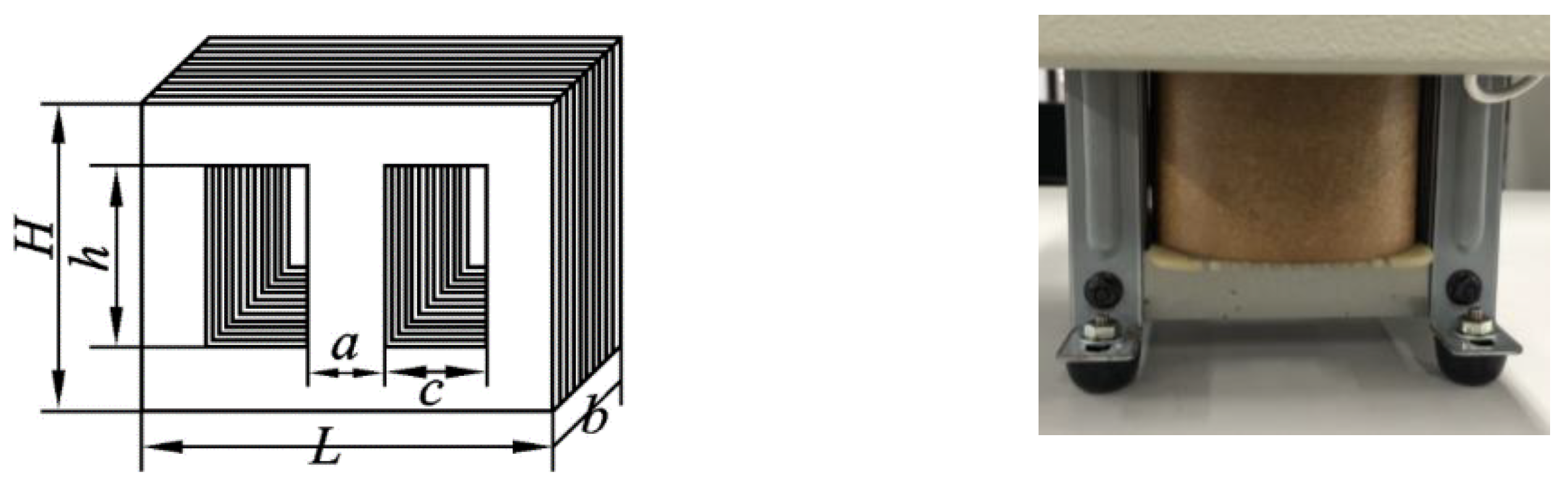
Disclaimer/Publisher’s Note: The statements, opinions and data contained in all publications are solely those of the individual author(s) and contributor(s) and not of MDPI and/or the editor(s). MDPI and/or the editor(s) disclaim responsibility for any injury to people or property resulting from any ideas, methods, instructions or products referred to in the content. |
© 2022 by the authors. Licensee MDPI, Basel, Switzerland. This article is an open access article distributed under the terms and conditions of the Creative Commons Attribution (CC BY) license (https://creativecommons.org/licenses/by/4.0/).