Finite-Time, Robust, and Adaptive Motion Control with State Constraints: Controller Derivation and Real Plant Experiments

Abstract

The paper refers to one of the most important problems in industrial automation and robotics—effective motion control in the presence of state variable constraints. A new, nonlinear, adaptive, robust, and practically applicable motion controller for a motor-driven servo is proposed. The developed controller guarantees that the transient of the motion is practically finished in a predefined time, and after this moment, the desired motion trajectory is tracked with specified accuracy, inviolable, time-variable constraints imposed on the position and the velocity are preserved, and all these features are robust against disturbances and violations of the system’s parameters. This approach, distinguished by the fact that the settling time and the quasi-steady-state tracking accuracy are explicitly available design parameters, has never been described before. The controller is based on a special type of time-varying barrier Lyapunov function (BLF), responsible for the finite-time tracking and for meeting the constraints. The derivation of the controller is based on Lyapunov stability theory. A mixture of robust adaptive, nonlinear control techniques is applied to prove the system’s stability. Numerous simulations and experiments with a real permanent-magnet motor- driven servo prove the practical applicability and usefulness of the presented approach.

1. Introduction

The main aim of this paper is to develop a new, nonlinear, adaptive, robust, and practically applicable controller for a motor-driven servo mechanism.

Servo drives are ubiquitous in numerous industrial applications, including CNC machines [1], robotic manipulators working in various industries including space applications [2], and all branches of industrial automation. Servo systems are commonly met in everyday life, starting from home and office automation to medical applications. There is no exaggeration in saying that the modern economy depends on the smooth running of the countless servo systems operating constantly around the world. A single, statistical servo consumes less energy than a single motor continuously propelling a manufacturing machine or a vehicle, but the great number of servos used means that the efficient control of each of them strongly influences global energy consumption and the energy efficiency of an industrial plant.

The main goal of each servo drive is to follow the assumed trajectory of motion (i.e., the desired position in time) with the prescribed accuracy. Practical implementation of the controlled servo usually requires that several additional conditions must be satisfied. State constraints must be preserved in any practically operating servo. In numerous applications, keeping the position and velocity inside hard constraints is a matter of safety. Moreover, the achievable control performance is limited by the specific features of the hardware. For instance, the finite encoder resolution limits the feasible tracking accuracy, and the highest possible propelling torque or force constrains the available acceleration. Therefore, all these practical conditions should be considered and included in the controller design procedure.

From a practical point of view, it is desirable that:

• the transient of the motion can be considered finished in the given time, which may be determined in advance;
• after this moment, the desired motion trajectory is tracked with a prescribed accuracy in the quasi-steady-state mode of the operation;
• all the time, starting from the initial conditions, during the transient and in the quasi-steady-state, the inviolable, time-variable constraints imposed on the position and the velocity are preserved;
• all these features are robust against violations of the system’s parameters and external disturbances.

The controller proposed in this paper guarantees that the above four conditions of the practical, finite-time servo control are met.

It is commonly accepted that a nonlinear load with unknown parameters, nonlinear friction, and the nonlinear characteristics of transmission devices are the main factors that affect the motion precision and may cause a risk of constraint violations. Therefore, it is commonly accepted that the nonlinear and adaptive control of servo systems outperforms the linear control techniques used in the previous century. The list of nonlinear control techniques applied for the servo control is almost endless. Some of them, recently used, include adaptive backstepping [3], numerous applications of neural networks [4], disturbances observers and compensation [5], sliding mode control [6], data-driven control [7], fractional controllers [8], learning control [9], model predictive control [10,11], and many others. Despite such vivid academic interest in the problem, new, improved, and practically applicable solutions are still needed. In particular, controllers guaranteeing practical finite-time control with full state constraints (in the sense defined by four postulates above) are still in demand.

State constraints may be achieved by a model predictive approach [12], but the two most prospective techniques are: (1) a nonlinear state transformation [13,14,15] and (2) the use of barrier Lyapunov functions (BLF) [16,17,18,19,20]. Constraints imposed on state variables may be constant [17] or changing in time [18,19,20]. A BLF approach usually requires some strict feasibility conditions.

The finite or fixed time control of nonlinear systems is based on the so-called semi-global practical finite-time stability conditions [21,22]. If the Lyapunov function $V$ is applied, this condition requires that the Lyapunov function derivative $\dot{V}$ fulfills the inequality $\dot{V}\le -\alpha V^p-\beta V^q+\rho$ where $\alpha >0,\beta >0,0<q<1,p\ge 1$. The unknown constant $\rho >0$ represents system uncertainties or disturbances and, if $\rho >0,$ although finite-time stability is guaranteed, the settling time and tracking accuracy depend on this unknown $\rho$. The Lyapunov function $V$ applied to prove finite-time stability can be a BLF, so finite-time control with state constraints is also possible [23,24]. Some recent results are presented in [25,26], but still, the achieved tracking accuracy depends on unknown system parameters and unstructured disturbances are not allowed. The settling time is a complicated function of design parameters and initial conditions, and it is difficult to define it in advance before checking complicated feasibility conditions.

The so-called funnel control [27,28] is an alternative to the BLF approach. This high-gain control is able to stabilize all systems of a certain class by using adjustable proportional gain and keeping the tracking error inside an exponential envelope. The tracking error achieves the final accuracy exponentially, not in a finite time [29,30,31].

The controller proposed in this paper offers design possibilities and guarantees a servo operation not available from the approaches described previously:

• a designer is able to impose a finite transient time and quasi-steady-state accuracy for the position tracking error as well as for the velocity tracking error;
• inviolable constraints around the desired position and velocity trajectory are met during the whole operation of the servo;
• the design is based on a simple servo model including nonlinearities with unknown parameters and unstructured disturbances with an unknown bound and the results are robust against these uncertainties.

Such features of the control system were achieved by using a specially designed BLF, responsible for the finite-time tracking and meeting the constraints at the same time. A similar BLF was used recently in [19] for the system output, and here it was applied for both state variables: position and velocity. Next, robust adaptive backstepping was applied to prove the system’s stability. The application of structured uncertainties in the plant model makes it possible to refer to the parameters corresponding exactly to the physical features of the real drive, such as inertia, viscous friction coefficient, etc. Corresponding adaptive parameters are therefore constrained in reasonable bounds—this was achieved by using robust adaptive laws with projection. The unstructured disturbance enabled the inclusion of all unmodelled phenomena. It was compensated by an adaptive control component, making the complete system robust.

All the features listed above contribute to the novelty of the proposed approach. Practical importance and applicability were proven by numerous experiments with the real plant reported in the paper.

In Section 2 the plant model selection is explained, and the control aims are formulated. The controller is developed in Section 3 and Section 4, and the system’s stability and parameter tuning are investigated in Section 5. Conclusions from the simulation experiments are presented in Section 6 and, finally, the experiments with a real servo are described, and the conclusions are given (Section 7).

2. Plant Model and Control Aims

The same universal model, based on the second principle of dynamics, can be used to describe a rotational or linear servo. Of course, the adequate meaning of signals and parameters must be observed. For instance, the term ‘position’ refers to an angular or a linear position, inertia denotes a moment of inertia or a mass, respectively, etc.

The first and the most important decision to be made while modelling the servo is to include or not include the motor dynamics in the model. Contemporary servo mechanisms are driven by rather fast motors, producing the desired torque or force almost instantly. In the case of electric propulsion, linear or rotational permanent magnet synchronous motors (PMSM) with pulse-with modulated (PWM) inverters are commonly used. In this case, torque or force is proportional to the motor current, and the current control loop time constant is usually at least 10 times smaller than the mechanical time constant. Therefore, it is reasonable to assume that the torque (force) is proportional to the control input of the drive. Of course, a gap exists between the demanded control and the real torque (force) developed by the motor. It may be caused by inevitable errors in the current control loop or by a cogging torque (force). However, this error may be included in the bounded, unstructured disturbance affecting the velocity dynamics, under the condition that the bound is finite, although not known. Although assuming that the torque (force) is proportional to a control input is obviously a relevant simplification, the real drive experiments presented in Section 7 prove that it allows satisfactory results to be obtained. An additional advantage of this assumption is that different types of drive (electric, pneumatic, hydraulic) can be considered within the same design approach.

Nonlinear friction strongly affects the performance of the servo. Usually, Coulomb and viscous-type friction dominate. Therefore, a dry plus viscous friction model with unknown parameters can be used, and the inevitable modelling inaccuracy can be included in the unstructured, bounded perturbation.

The main load, caused by the machine being moved by the servo, or by gravitation affecting the motion of a manipulator, or any other reasons, is modeled as a linear combination of known nonlinear functions of position and velocity, with unknown parameters. Such structured uncertainty enables an effective compensation of the forces acting against the motion.

As a result, a rotational or a linear servo is modeled by ordinary differential equations:

$$\begin{gathered} {\dot{x}}_1=x_2, \\ \overline{m}{\dot{x}}_2=\tau -\overline{F}-\overline{L}+\overline{d} \end{gathered}$$

(1)

where $x_1$ denotes the linear or rotational position, $x_2$ stands for the linear or rotational speed, and $\overline{m}$ represents inertia (mass for linear motion, moment of inertia in case of rotational motion). The input $\tau$ signifies the propelling force or torque. The main part of the load is described by a linear combination of known functions $\mathrm{S}\left(x_1,x_2\right)={\left[\begin{array}{cc}\begin{array}{cc}{\mathrm{S}}_1\left(x_1,x_2\right)& {\mathrm{S}}_2\left(x_1,x_2\right)\end{array}& \begin{array}{cc}\cdots & {\mathrm{S}}_p\left(x_1,x_2\right)\end{array}\end{array}\right]}^T$ with $p$ unknown parameters $\overline{c}=\left[\begin{array}{ccc}{\overline{c}}_1& \cdots & {\overline{c}}_p\end{array}\right]$, while a friction force or torque is approximated by a dry plus viscous friction model:

$$\overline{L}={\overline{c}}^T\mathrm{S}\left(x_1,x_2\right), \overline{F}=\overline{b}{x}_2+\overline{T}sign\left(x_2\right).$$

(2)

It is assumed that all model parameters $\overline{m}, \overline{c}, \overline{b},\overline{ T}$ are unknown, although some inaccurate initial or nominal values ${\overline{m}}_0$, ${\overline{c}}_0, {\overline{b}}_0$, ${\overline{T}}_0$ are available. As the used model parameters correspond to real, physical parameters of the drive, it is possible to propose reasonable constraints for the unknown values.

Any load modelling errors and the effects of imperfect realization of the control signal are represented by an unstructured disturbance $\overline{d}$. It is assumed that this disturbance is bounded:

$$\left|\overline{d}\left(t\right)\right|\le {\overline{D}}_M,$$

(3)

although the constraint ${\overline{D}}_M$ is unknown.

Usually, the input $\tau$ is not directly available, but it is proportional to a real control input $I$. For electric-driven servos, this input is a motor current (quadratic axis current for PMSMs) and for hydraulic or pneumatic servos it is a resultant pressure acting on the piston. Therefore,

$$\tau =K_{\tau }I,$$

(4)

where $I$ is the control input. The coefficient of proportionality is not known exactly, although it is strictly positive, and some reasonable bounds can be guessed.

After plugging (4) into (1) and dividing by $K_{\tau }$ the final model of the servo is obtained:

$$\begin{gathered} {\dot{x}}_1=x_2, \\ m{\dot{x}}_2=I-F-L+d, \\ L=c^T\mathrm{S}\left(x_1,x_2\right), F=b{x}_2+Tsign\left(x_2\right), \left|d\left(t\right)\right|\le D_M, \end{gathered}$$

(5)

where $\left[m c^T b T D_M\right]=\frac{1}{K_{\tau }}\left[\overline{m} {\overline{c}}^T \overline{b} \overline{ T} {\overline{D}}_M\right]$ and $m_0, c_0, b_0, T_0$ are inaccurate initial or nominal values for $m, c, b, T.$

The servo is supposed to track a smooth desired position trajectory $x_{1d}$ with the predefined accuracy ${\epsilon }_1$ and this control aim must be achieved in the prescribed time $T_1$. So, the tracking error:

$$e_1:=x_{1d}-x_1$$

(6)

has to fulfill

$$\forall t>T_1 \left|e_1\left(t\right)\right|\le {\epsilon }_1.$$

(7)

It is assumed that the desired trajectory is bounded by time-varying constraints and the servo position must be kept inside the same hard constraints during the complete transient:

$$x_{1m}\left(t\right)\le x_{1d}\left(t\right)\le x_{1M}\left(t\right),\hspace{1em}{x}_{1m}\left(t\right)\le x_1\left(t\right)\le x_{1M}\left(t\right).$$

(8)

It follows from (8) that:

$$\left|e_1\left(t\right)\right|\le x_{1M}\left(t\right)-x_{1m}\left(t\right).$$

(9)

The constraints and the control aims must be consistent and feasible, therefore it is assumed that:

• the set of available initial positions is bounded, such that

  $$\left|e_1\left(0\right)\right|\le R,$$

  (10)
• there exists a smooth, positive function $B_1\left(t\right)$, such that

  $$x_{1m}\left(t\right)\le x_{1d}\left(t\right)-B_1\left(t\right)<x_{1d}\left(t\right)+B_1\left(t\right)\le x_{1M}\left(t\right)$$

  (11)

  and

  $$B_1\left(0\right)\ge R, \forall t\ge T_1 B_1\left(t\right)\le {\epsilon }_1.$$

  (12)

This function is supposed to constrain the tracking error. The tracking error ${\epsilon }_1$ should be achieved after the time $T_1$ and ${\epsilon }_1, T_1$ are design parameters.

The specified control aims must be accomplished by a practically realizable control, so it is realistic to assume that the servo speed is limited. Of course, the desired motion velocity must remain inside these limits. The servo must be faster than the desired motion to achieve tracking, hence it is reasonable to demand that:

$$\begin{array}{c}\left|x_2\right|\le \left|{\dot{x}}_{1d}\right|+\Delta \end{array}.$$

(13)

The desired “speed advantage” $\Delta$ must be precisely defined during the controller design and be connected with the choice of controller parameters.

3. Time-Varying Barrier Function to Achieve Position Tracking

Let us consider any twice continuously differentiable function $B_1\left(t\right)$, fulfilling conditions (11) and (12). According to (10), it follows from (12) that:

$$\left|e_1\left(0\right)\right|\le \begin{array}{c}{B}_1\left(0\right)\end{array}$$

(14)

and the finite-time tracking will be achieved by making $\left|e_1\left(t\right)\right|\le \begin{array}{c}{B}_1\left(t\right)\end{array}$ for any $t$. An example of a function fulfilling all above requirements is:

$$B_1\left(t\right)=\{\begin{array}{cc}r{\left(\sin \left(\frac{\pi }{2T_1}\left(T_1-t\right)\right)\right)}^3+{\epsilon }_1& t\le T_1\\ {\epsilon }_1& t>T_1\end{array}$$

(15)

with

$$r=R-{\epsilon }_1.$$

(16)

This is plotted in Figure 1a. A typical configuration of the desired trajectory and the constraints is presented in Figure 1b.

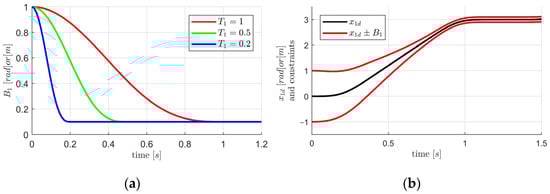
Figure 1. Function (16) for different parameters $T_1$ (${\epsilon }_1=0.1, r=1)$ (a) and an example of a desired position trajectory inside the constraints ($T_1=1, {\epsilon }_1=0.1, r=1)$ (b).

The first derivative of $B_1$ is continuous and given by:

$${\dot{B}}_1\left(t\right)=\{\begin{array}{cc}-\frac{3\pi }{2T_1}r{\sin }^2\left(\frac{\pi }{2T_1}\left(T_1-t\right)\right)\cos \left(\frac{\pi }{2T_1}\left(T_1-t\right)\right)& t\le T_1\\ 0& t>T_1\end{array}$$

(17)

Note that ${\dot{B}}_1\left(0\right)={\dot{B}}_1\left(T_1\right)=0, \left|{\dot{B}}_1\left(t\right)\right|\le \frac{3\pi }{2T_1}r\frac{2}{3\sqrt{3}}=\frac{\pi }{\sqrt{3}{T}_1}r$.

The boundedness of the tracking error is obtained with the use of the Lyapunov barrier function:

$$V_1=\frac{1}{2}{\mathrm{A}}_1^2, \hspace{1em}{\mathrm{A}}_1=\frac{B_1^2{e}_1}{B_1^2-e_1^2}.$$

(18)

Because of (14), $V_1\left(e_1\left(0\right)\right)$ is finite, $V_1\left(e_1\left(t\right)\right)$ remains bounded if $\left|e_x\left(t\right)\right|<\begin{array}{c}{B}_x\left(t\right)\end{array}$ and tends to the infinity if $\left|e_1\left(t\right)\right|\to \begin{array}{c}{B}_1\left(t\right)\end{array}$. Exemplary isolines of $V_1$ are plotted in Figure 2.

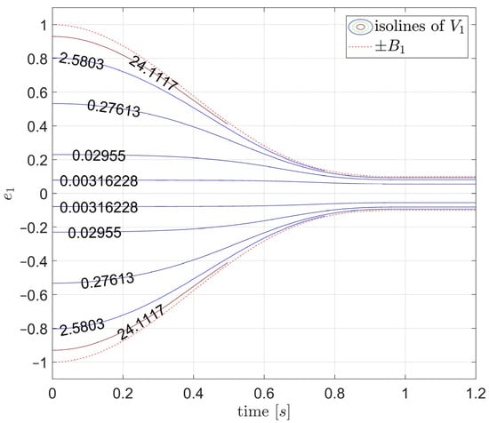
Figure 2. Exemplary isolines of $V_1$ and the constraint $\pm B_1\left(t\right)$.

The satisfactory behavior of $e_1$ is assured by designing the adequate transient of the servo velocity. The desired speed trajectory is denoted by $x_{2d}$ and the speed tracking error is:

$$e_2:=x_{2d}-x_2.$$

(19)

Therefore, the position tracking error dynamics is described as:

$${\dot{e}}_1={\dot{x}}_{1d}-x_2={\dot{x}}_{1d}-x_{2d}+e_2.$$

(20)

The derivative of the Lyapunov function along the system trajectory is calculated as:

$${\dot{V}}_1={\mathrm{A}}_1{\dot{\mathrm{A}}}_1={\mathrm{A}}_1\left(\frac{\partial {\mathrm{A}}_1}{\partial B_1}{\dot{B}}_1+\frac{\partial {\mathrm{A}}_1}{\partial e_1}{\dot{e}}_1\right).$$

(21)

After defining functions:

$$C_1=\frac{\partial {\mathrm{A}}_1}{\partial B_1}{\dot{B}}_1=\frac{-2B_1{e}_1^3}{{\left(B_1^2-e_1^2\right)}^2}{\dot{B}}_1,$$

(22)

$$D_1=\frac{\partial {\mathrm{A}}_1}{\partial e_1}=\frac{B_1^2\left(B_1^2+e_1^2\right)}{{\left(B_1^2-e_1^2\right)}^2},$$

(23)

$$E_1=\frac{C_1}{D_1}=\frac{-2e_1^3}{B_1\left(B_1^2+e_1^2\right)}{\dot{B}}_1,$$

(24)

(Note that $D_1>0$ for any $e_1$) and using (20), the expression (21) is transferred into:

$$\begin{array}{c}{\dot{V}}_1={\mathrm{A}}_1{\dot{\mathrm{A}}}_1={\mathrm{A}}_1\left(C_1+D_1{\dot{e}}_1\right)={\mathrm{A}}_1\left(C_1+D_1{\dot{x}}_{1d}-D_1{x}_2\right)\\ ={\mathrm{A}}_1\left(C_1+D_1{\dot{x}}_{1d}-D_1{x}_{2d}+D_1{e}_2\right)={\mathrm{A}}_1{D}_1\left(\frac{C_1}{D_1}+{\dot{x}}_{1d}-x_{2d}+e_2\right)\\ ={\mathrm{A}}_1{D}_1\left(E_1+{\dot{x}}_{1d}-x_{2d}+e_2\right).\end{array}$$

(25)

Hence, selecting the desired velocity as:

$$x_{2d}={\dot{x}}_{1d}+E_1+\frac{k_1}{D_1}{\mathrm{A}}_1={\dot{x}}_{1d}+\frac{-2e_1^3}{B_1\left(B_1^2+e_1^2\right)}{\dot{B}}_1+k_1\frac{e_1\left(B_1^2-e_1^2\right)}{B_1^2+e_1^2},$$

(26)

where $k_1>0$ is the design parameter, results in:

$$\begin{array}{c}{\dot{V}}_1=-k_1{\mathrm{A}}_1^2+{\mathrm{A}}_1{D}_1{e}_2\end{array}.$$

(27)

Hence, if $e_2\to 0$ then ${\dot{V}}_1$ becomes negative. The specific value of $k_1$ must be selected to assure that:

$$x_{2d}\left(0\right)={\dot{x}}_d\left(0\right)+k_1\frac{e_1\left(0\right)\left(R^2-e_1^2\left(0\right)\right)}{R^2+e_1^2\left(0\right)}$$

(28)

satisfies

$$x_{2m}\le x_{2d}\left(0\right)\le x_{2M},$$

(29)

where $x_{2m}, x_{2M}$ denote predefined initial speed constraints. Obviously, the same constraints are accomplished by an initial speed value:

$$x_{2m}\le x_2\left(0\right)\le x_{2M}.$$

(30)

4. Velocity Control Loop

According to (5), the velocity error dynamics are given by:

$$m{\dot{e}}_2=m{\dot{x}}_{2d}-m{\dot{x}}_2=m{\dot{x}}_{2d}-I+b{x}_2+Tsign\left(x_2\right)+c^T\mathrm{S}\left(x_1,x_2\right)-d\left(t\right)$$

(31)

and because of (29) and (30) the initial value is bounded by:

$$\left|e_2\left(0\right)\right|\le x_{2M}-x_{2m}.$$

(32)

The velocity error should be constrained by a barrier function, similar to the one used in the position control loop. The velocity barrier function is selected as:

$$B_2=\{\begin{array}{cc}q{\sin }^2\left(\frac{\pi }{2T_2}\left(T_2-t\right)\right)+{\epsilon }_2& t\le T_2\\ {\epsilon }_2& t>T_2\end{array}$$

(33)

with

$$q\ge x_{2M}-x_{2m}-{\epsilon }_2$$

(34)

and parameters ${\epsilon }_2$ (defining the tracking accuracy) and $T_2$ (defining the settling time).

The unknown parameters $m$, $b$, $T$, $c$ and $D_M$ must be substituted by adaptive parameters $\widehat{m}$, $\widehat{b}$, $\widehat{T}$, $\widehat{c}$ and ${\widehat{D}}_M$ and the adaptation errors are denoted by:

$$\tilde{m}=m-\widehat{m},$$

(35)

$$\tilde{b}=b-\widehat{b},$$

(36)

$$\tilde{T}=T-\widehat{T},$$

(37)

$$\tilde{c}=c-\widehat{c}.$$

(38)

$${\tilde{D}}_M=D_M-{\widehat{D}}_M.$$

(39)

The Lyapunov function for the complete closed-loop system should contain all dynamic variables. Therefore, it is selected as:

$$V_2=V_1+\frac{1}{2}m{\mathrm{A}}_2^2+\frac{1}{2{\gamma }_m}{\tilde{m}}^2+\frac{1}{2{\gamma }_b}{\tilde{b}}^2+\frac{1}{2{\gamma }_T}{\tilde{T}}^2+\frac{1}{2}{\tilde{c}}^T{\gamma }_c^{-1}\tilde{c}+\frac{1}{2{\gamma }_D}{\tilde{D}}_M^2$$

(40)

with

$${\mathrm{A}}_2=\frac{B_2^2{e}_2}{B_2^2-e_2^2}$$

(41)

and the design parameters: positive ${\gamma }_m, {\gamma }_b, {\gamma }_T, {\gamma }_D$ positive definite matrix ${\gamma }_c$.

Derivation of the Lyapunov function derivative ${\dot{V}}_2$ requires the calculation of:

$${\dot{B}}_2\left(t\right)=\{\begin{array}{cc}-\frac{\pi }{T_2}q\sin \left(\frac{\pi }{2T_2}\left(T_2-t\right)\right)\cos \left(\frac{\pi }{2T_2}\left(T_2-t\right)\right)& t\le T_2\\ 0& t>T_2\end{array}$$

(42)

and

$$C_2=\frac{\partial {\mathrm{A}}_2}{\partial B_2}{\dot{B}}_2=\frac{-2B_2{e}_{v2}^3}{{\left(B_2^2-e_2^2\right)}^2}{\dot{B}}_2,$$

(43)

$$D_2=\frac{\partial {\mathrm{A}}_2}{\partial e_2}=\frac{B_2^2\left(B_2^2+e_2^2\right)}{{\left(B_2^2-e_2^2\right)}^2},$$

(44)

$$E_2=\frac{C_2}{D_2}=\frac{-2e_2^3}{B_2\left(B_2^2+e_2^2\right)}{\dot{B}}_2,$$

(45)

$$F_2=\frac{e_2}{{\mathrm{A}}_2{D}_2}=\frac{{\left(B_2^2-e_2^2\right)}^3}{B_2^4\left(B_2^2+e_2^2\right)}$$

(46)

(Note that $D_2>0$and $\frac{{\mathrm{A}}_2}{e_2}>0$). Expressions (42)–(46) and (31) allow us to represent the Lyapunov function derivative as:

$$\begin{array}{cc}{\dot{V}}_2\hfill & ={\dot{V}}_1+m{\mathrm{A}}_2{\dot{\mathrm{A}}}_2+\frac{1}{{\gamma }_m}\tilde{m}\dot{\tilde{m}}+\frac{1}{{\gamma }_b}\tilde{b}\tilde{b}+\frac{1}{{\gamma }_T}\tilde{T}\dot{\tilde{T}}+{\tilde{c}}^T{\gamma }_c^{-1}\dot{\tilde{c}}+\frac{1}{{\gamma }_D}{\tilde{D}}_M{\dot{\tilde{D}}}_M\hfill \\ & =-k_1{\mathrm{A}}_1^2+{\mathrm{A}}_1{D}_1{e}_2+{\mathrm{A}}_2\left(m{C}_2+m{D}_2{\dot{e}}_2\right)-\frac{1}{{\gamma }_m}\tilde{m}\dot{\widehat{m}}-\frac{1}{{\gamma }_b}\tilde{b}\dot{\widehat{b}}-\frac{1}{{\gamma }_T}\tilde{T}\dot{\widehat{T}}-{\tilde{c}}^T{\gamma }_c^{-1}\dot{\widehat{C}}-\frac{1}{{\gamma }_D}{\tilde{D}}_M{\dot{\widehat{D}}}_M\hfill \\ & =-k_1{\mathrm{A}}_1^2+{\mathrm{A}}_1{D}_1{e}_2+{\mathrm{A}}_2\left(m{C}_2+D_2\left[m{\dot{x}}_{2d}-I+b{x}_2+Tsign\left(x_2\right)+c^T\mathrm{S}\left(x_1,x_2\right)-d\left(t\right)\right]\right)\hfill \\ & \hspace{1em}\hspace{1em}\hspace{1em}\hspace{1em}\hspace{1em}-\frac{1}{{\gamma }_m}\tilde{m}\dot{\widehat{m}}-\frac{1}{{\gamma }_b}\tilde{b}\dot{\widehat{b}}-\frac{1}{{\gamma }_T}\tilde{T}\dot{\widehat{T}}-{\tilde{c}}^T{\gamma }_c^{-1}\dot{\widehat{c}}-\frac{1}{{\gamma }_D}{\tilde{D}}_M{\dot{\widehat{D}}}_M\hfill \\ & =-k_1{\mathrm{A}}_1^2+{\mathrm{A}}_1{D}_1{e}_2+{\mathrm{A}}_2{D}_2\left(m{E}_2+m{\dot{x}}_{2d}-I+b{x}_2+Tsign\left(x_2\right)+c^T\mathrm{S}\left(x_1,x_2\right)-d\left(t\right)\right)\hfill \\ & \hspace{1em}\hspace{1em}\hspace{1em}\hspace{1em}\hspace{1em}-\frac{1}{{\gamma }_m}\tilde{m}\dot{\widehat{m}}-\frac{1}{{\gamma }_b}\tilde{b}\dot{\widehat{b}}-\frac{1}{{\gamma }_T}\tilde{T}\dot{\widehat{T}}-{\tilde{c}}^T{\gamma }_c^{-1}\dot{\widehat{c}}-\frac{1}{{\gamma }_D}{\tilde{D}}_M{\dot{\widehat{D}}}_M\hfill \\ & =-k_1{\mathrm{A}}_1^2+{\mathrm{A}}_2{D}_2\left\{{\mathrm{A}}_1{D}_1{F}_2+m{E}_2+m{\dot{x}}_{2d}-I+b{x}_2+Tsign\left(x_2\right)+c^T\mathrm{S}\left(x_1,x_2\right)-d\left(t\right)\right\}\hfill \\ & \hspace{1em}\hspace{1em}\hspace{1em}\hspace{1em}\hspace{1em}-\frac{1}{{\gamma }_m}\tilde{m}\dot{\widehat{m}}-\frac{1}{{\gamma }_b}\tilde{b}\dot{\widehat{b}}-\frac{1}{{\gamma }_T}\tilde{T}\dot{\widehat{T}}-{\tilde{c}}^T{\gamma }_c^{-1}\dot{\widehat{c}}-\frac{1}{{\gamma }_D}{\tilde{D}}_M{\dot{\widehat{D}}}_M\hfill \\ & =-k_1{\mathrm{A}}_1^2+{\mathrm{A}}_2{D}_2\left\{{\mathrm{A}}_1{D}_1{F}_2+(\tilde{m}+\widehat{m})\left(E_2+{\dot{x}}_{2d}\right)-I+(\tilde{b}+\widehat{b})x_2+(\tilde{T}+\widehat{T})sign\left(x_2\right)+{(\tilde{c}+\widehat{c})}^T\mathrm{S}\left(x_1,x_2\right)-d\left(t\right)\right\}\hfill \\ & \hspace{1em}\hspace{1em}\hspace{1em}\hspace{1em}\hspace{1em}-\frac{1}{{\gamma }_m}\tilde{m}\dot{\widehat{m}}-\frac{1}{{\gamma }_b}\tilde{b}\dot{\widehat{b}}-\frac{1}{{\gamma }_T}\tilde{T}\dot{\widehat{T}}-{\tilde{c}}^T{\gamma }_c^{-1}\dot{\widehat{c}}-\frac{1}{{\gamma }_D}{\tilde{D}}_M{\dot{\widehat{D}}}_M.\hfill \end{array}$$

(47)

Therefore, the control law:

$$I=D_1{\mathrm{A}}_1{F}_2+\widehat{m}\left(E_2+{\dot{x}}_{2d}\right)+\widehat{b}{x}_2+\widehat{T}sign\left(x_2\right)+{\widehat{c}}^T\mathrm{S}\left(x_1,x_2\right)+\frac{k_2}{D_2}{\mathrm{A}}_2-{\widehat{D}}_M\tanh \left(\frac{D_2{\mathrm{A}}_2}{\kappa }\right)$$

(48)

reduces (47) into

$$\begin{array}{l}{\dot{V}}_2=-k_1{\mathrm{A}}_1^2-k_2{\mathrm{A}}_2^2+{\mathrm{A}}_2{D}_2\left\{\tilde{m}\left(E_2+{\dot{x}}_{2d}\right)+\tilde{b}{x}_2+\tilde{T}sign\left(x_2\right)+{\tilde{c}}^T\mathrm{S}\left(x_1,x_2\right)-d\left(t\right)-{\widehat{D}}_M\tanh \left(\frac{D_2{\mathrm{A}}_2}{\kappa }\right)\right\}\\ \hspace{1em}\hspace{1em}\hspace{1em}\hspace{1em}\hspace{1em}\hspace{1em}-\frac{1}{{\gamma }_m}\tilde{m}\dot{\widehat{m}}-\frac{1}{{\gamma }_b}\tilde{b}\dot{\widehat{b}}-\frac{1}{{\gamma }_T}\tilde{T}\dot{\widehat{T}}-{\tilde{c}}^T{\gamma }_c^{-1}\dot{\widehat{c}}-\frac{1}{{\gamma }_D}{\tilde{D}}_M{\dot{\widehat{D}}}_M.\end{array}$$

(49)

The derivative of the desired velocity ${\dot{x}}_{2d}$, required in the control law (48), may be obtained by differentiating (26):

$$\begin{array}{c}{\dot{x}}_{2d}={\ddot{x}}_{1d}-\frac{2e_1^3}{B_1\left(B_1^2+e_1^2\right)}{\ddot{B}}_1+\frac{\partial x_{2d}}{\partial B_1}{\dot{B}}_1+\frac{\partial x_{2d}}{\partial e_1}{\dot{e}}_1={\ddot{x}}_{1d}-\frac{2e_1^3}{B_1\left(B_1^2+e_1^2\right)}{\ddot{B}}_1\\ +\frac{2e_1^3\left(3B_1^2+e_1^2\right)+4k_1{B}_1^3{e}_1^3}{B_1^2{\left(B_1^2+e_1^2\right)}^2}{\dot{B}}_1-\frac{2B_1{e}_1^2\left(3B_1^2+2e_1^2\right)+k_1{e}_1^2{B}_1^2\left(5B_1^2-e_1^2\right)}{B_1^2{\left(B_1^2+e_1^2\right)}^2}{\dot{e}}_1\end{array}$$

(50)

Finally, adaptive laws must be selected. Implementation in the real, physical system requires that the so-called robust adaptive laws [32] must be applied. As the adaptive parameters $\widehat{m},\widehat{c},\widehat{b},\widehat{T}$ correspond to physical plant parameters $m, c, b, T$, it is reasonable to keep their values somewhere around the expected values. Although the identification or tracking of real parameters by their adaptive counterparts is not necessary for the stability of the closed-loop system and the realization of the control aims, it is well known that large deviations of adaptive parameters may cause higher control values. It is particularly important that negative values of the adaptive parameters are avoided, as the real parameters $m, b, T, c$ are positive. Therefore, adaptive laws using a projection operator with pre-defined bounds are selected. The constraints for adaptive parameters are defined by the following set of inequalities:

$$m^m\le \widehat{m}\le m^M,$$

(51)

$$b^m\le \widehat{b}\le b^M,$$

(52)

$$T^m\le \widehat{T}\le T^M,$$

(53)

$$c_i^m\le {\widehat{c}}_i\le c_i^M, i=1,\dots ,p,$$

(54)

where $m^M$, $m^m$, $b^M$, $b^m$, $T^M$, $T^m$, $c_i^m$, $c_i^M$ are constant parameters, which may be deduced from the available inaccurate or nominal values $m_0$, $b_0, T_0, c_0,$and the expected range of changes of plant parameters. Of course, it is assumed that these nominal parameters and real parameters $m, b, T, c$ fulfill the same constraints (51)–(54) as well.

Robust adaptive laws using the projection operator are defined by the differential equations:

$$\dot{\widehat{m}}={\mathrm{proj}}_{m^m,m^M}\left({\gamma }_m{\mathrm{A}}_2{D}_2\left(E_2+{\dot{x}}_{2d}\right),\widehat{m}\right),$$

(55)

$$\dot{\widehat{b}}={\mathrm{proj}}_{b^m,b^M}\left({\gamma }_b{\mathrm{A}}_2{D}_2{x}_2,\widehat{b}\right),$$

(56)

$$\dot{\widehat{T}}={\mathrm{proj}}_{T^m,T^M}\left({\gamma }_T{\mathrm{A}}_2{D}_{2}sign\left(x_2\right),\widehat{T}\right),$$

(57)

$$\dot{\widehat{c}}={\mathrm{proj}}_{c^m,c^M}\left({\gamma }_c{\mathrm{A}}_2{D}_2\mathrm{S}\left(x_1,x_2\right),\widehat{c}\right),$$

(58)

where for scalar arguments ${\alpha }^m,{\alpha }^M, \beta ,\widehat{p}\in ℝ$

$${\mathrm{proj}}_{{\alpha }^m,{\alpha }^M}\left(\beta ,\widehat{p}\right)=\{\begin{array}{c}0 \mathrm{if} \widehat{p}\le {\alpha }^m \mathrm{and} \beta <0\\ 0 \mathrm{if} \widehat{p}\ge {\alpha }^M \mathrm{and} \beta >0\\ \beta \mathrm{in} \mathrm{any} \mathrm{other} \mathrm{case}\end{array},$$

(59)

and for vectors ${\alpha }^m,{\alpha }^M, \beta ,\widehat{p}\in {ℝ}^r$

$$\begin{array}{l}{\mathrm{proj}}_{{\alpha }^m,{\alpha }^M}\left(\beta ,\widehat{p}\right)\\ ={\left[\begin{array}{cc}\begin{array}{cc}{\mathrm{proj}}_{{\alpha }_1^m,{\alpha }_1^M}\left({\beta }_1,{\widehat{p}}_1\right)& {\mathrm{proj}}_{{\alpha }_2^m,{\alpha }_2^M}\left({\beta }_2,{\widehat{p}}_2\right)\end{array}& \begin{array}{cc}\cdots & {\mathrm{proj}}_{{\alpha }_r^m,{\alpha }_r^M}\left({\beta }_r,{\widehat{p}}_r\right)\end{array}\end{array}\right]}^T.\end{array}$$

(60)

The last adaptive parameter ${\widehat{D}}_M$ corresponds to the unknown, maximal norm of the unstructured disturbance $D_M$ introduced in (5). The adaptive law is defined as:

$${\dot{\widehat{D}}}_M={\gamma }_D\left({\mathrm{A}}_2{D}_2\tanh \left(\frac{{\mathrm{A}}_2{D}_2}{\kappa }\right)-{\sigma }_D\Vert \mathrm{A}\Vert \left({\widehat{D}}_M-D_{M0}\right)\right),$$

(61)

where $\Vert \mathrm{A}\Vert =\sqrt{{\mathrm{A}}_1^2+{\mathrm{A}}_2^2}$, $D_{M0}$ is an initial guess or nominal value of unknown parameter, $\kappa >0$ and ${\sigma }_D$ is a positive parameter making the adaptive law robust. It follows from this adaptive law that ${\widehat{D}}_M\left(t\right)$ is a non-decreasing function of time.

Under adaptive laws (55)–(58) and (61), taking into account that:

• $D_2>0$;
• for any real $\omega$ and $\rho >0$, $0\le \left|\omega \right|-\omega \tanh \frac{\omega }{\rho }\le 0.2785\rho$ [19], so $\left|{\mathrm{A}}_2\right|D_2{D}_M-{\mathrm{A}}_2{D}_2{D}_M\tanh \left(\frac{{\mathrm{A}}_2{D}_2}{\kappa }\right)=\left|{\mathrm{A}}_2\right|D_2{D}_M-{\mathrm{A}}_2{D}_2{D}_M\tanh \left(\frac{{\mathrm{A}}_2{D}_2{D}_M}{\kappa D_M}\right)\le 0.2785\kappa D_M$;
• for any scalar $\gamma >0$ ${\mathrm{proj}}_{{\alpha }^m,{\alpha }^M}\left(\gamma \beta ,\widehat{p}\right)=\gamma {\mathrm{proj}}_{{\alpha }^m,{\alpha }^M}\left(\beta ,\widehat{p}\right)$;
• for any $\alpha$ such that ${\alpha }^m\le \alpha \le {\alpha }^M$, the inequality $\left(\alpha -\widehat{p}\right)\left(\beta -{\mathrm{proj}}_{{\alpha }^m,{\alpha }^M}\left(\beta ,\widehat{p}\right)\right)\le 0$ holds [33].

The Lyapunov function derivative is reduced:

$$\begin{array}{c}{\dot{V}}_2=-k_1{\mathrm{A}}_1^2-k_2{\mathrm{A}}_2^2+\tilde{m}{\mathrm{A}}_2{D}_2\left(E_2+{\dot{x}}_{2d}\right)+\tilde{b}{\mathrm{A}}_2{D}_2{x}_2+\tilde{T}{\mathrm{A}}_2{D}_{2}sign\left(x_2\right)+{\tilde{c}}^T{\mathrm{A}}_2{D}_2\mathrm{S}\left(x_1,x_2\right)-{\mathrm{A}}_2{D}_{2}d\left(t\right)\\ -{\mathrm{A}}_2{D}_2{\widehat{D}}_{M}tanh\left(\frac{D_2{\mathrm{A}}_2}{\kappa }\right)-\frac{1}{{\gamma }_m}\tilde{m}{proj}_{m^m,m^M}\left({\gamma }_m{\mathrm{A}}_2{D}_2\left(E_2+{\dot{x}}_{2d}\right),\widehat{m}\right)-\frac{1}{{\gamma }_b}\tilde{b}{proj}_{b^m,b^M}\left({\gamma }_b{\mathrm{A}}_2{D}_2{x}_2,\widehat{b}\right)\\ -\frac{1}{{\gamma }_T}\tilde{T}{proj}_{T^m,T^M}\left({\gamma }_T{\mathrm{A}}_2{D}_{2}sign\left(x_2\right),\widehat{T}\right)-{\tilde{c}}^T{\gamma }_c^{-1}{Proj}_{c^m,c^M}\left({\gamma }_c{\mathrm{A}}_2{D}_2\mathrm{S}\left(x_1,x_2\right),\widehat{c}\right)-{\tilde{D}}_M{\mathrm{A}}_2{D}_{2}tanh\left(\frac{{\mathrm{A}}_2{D}_2}{\kappa }\right)\\ +{\sigma }_D\parallel \mathrm{A}\parallel {\tilde{D}}_M\left({\widehat{D}}_M-D_{M0}\right)\le -k_1{\mathrm{A}}_1^2-k_2{\mathrm{A}}_2^2+\tilde{m}{\mathrm{A}}_2{D}_2\left(E_2+{\dot{x}}_{2d}\right)+\tilde{b}{\mathrm{A}}_2{D}_2{x}_2+\tilde{T}{\mathrm{A}}_2{D}_{2}sign\left(x_2\right)\\ +{\tilde{c}}^T{\mathrm{A}}_2{D}_2\mathrm{S}\left(x_1,x_2\right)-{\mathrm{A}}_2{D}_{2}d\left(t\right)-{\mathrm{A}}_2{D}_2{\widehat{D}}_{M}tanh\left(\frac{D_2{\mathrm{A}}_2}{\kappa }\right)-\tilde{m}{proj}_{m^m,m^M}\left({\mathrm{A}}_2{D}_2\left(E_2+{\dot{x}}_{2d}\right),\widehat{m}\right)\\ -\tilde{b}{proj}_{b^m,b^M}\left({\mathrm{A}}_2{D}_2{x}_2,\widehat{b}\right)-\tilde{T}{proj}_{T^m,T^M}\left({\mathrm{A}}_2{D}_{2}sign\left(x_2\right),\widehat{T}\right)-{\tilde{c}}^T{Proj}_c^m,c^M\left({\mathrm{A}}_2{D}_2\mathrm{S}\left(x_1,x_2\right),\widehat{c}\right)\\ -{\tilde{D}}_M{\mathrm{A}}_2{D}_{2}tanh\left(\frac{{\mathrm{A}}_2{D}_2}{\kappa }\right)+{\sigma }_D\parallel \mathrm{A}\parallel {\tilde{D}}_M\left({\widehat{D}}_M-D_{M0}\right)\le -k_1{\mathrm{A}}_1^2-k_2{\mathrm{A}}_2^2\\ +\tilde{T}\left({\mathrm{A}}_2{D}_{2}sign\left(x_2\right)-{proj}_T^m,T^M\left({\mathrm{A}}_2{D}_{2}sign\left(x_2\right),\widehat{T}\right)\right)+{\tilde{c}}^T\left({\mathrm{A}}_2{D}_2\mathrm{S}\left(x_1,x_2\right)-{Proj}_{c^m,c^M}\left({\mathrm{A}}_2{D}_2\mathrm{S}\left(x_1,x_2\right),\widehat{c}\right)\right)\\ +\left|{\mathrm{A}}_2\right|D_2{D}_M-{\mathrm{A}}_2{D}_2{D}_{M}tanh\left(\frac{{\mathrm{A}}_2{D}_2}{\kappa }\right)+{\sigma }_D\parallel \mathrm{A}\parallel {\tilde{D}}_M\left(-{\tilde{D}}_M+D_M-D_{M0}\right)\\ \le -k_1{\mathrm{A}}_1^2-k_2{\mathrm{A}}_2^2-\frac{{\sigma }_D}{2}\parallel \mathrm{A}\parallel {\tilde{D}}_M^2+\frac{{\sigma }_D}{2}\parallel \mathrm{A}\parallel {\left(D_M-D_{M0}\right)}^2+0.2785D_M\kappa .\end{array}$$

(62)

The closed-loop controller consists of:

• the desired velocity trajectory (26) and its derivative (50);
• the control law (48);
• the adaptive laws (55)–(58), (61).

The designer selects:

• the parameters of the constraints: $r, T_1, {\epsilon }_1$ in (15) and $q, T_2, {\epsilon }_2$ in (33);
• the controller gains: $k_1$ in (26), $k_2$ and $\kappa$ in (48);
• the adaptation gains ${\gamma }_m, {\gamma }_b, {\gamma }_T, {\gamma }_D$ and ${\gamma }_c$, and the ‘robustifying’ parameter ${\sigma }_D$ in (61);
• the projection constraints $m^M$, $m^m$, $b^M$, $b^m$, $T^M$, $T^m$, $c_i^m$, $c_i^M$;
• the initial values of adaptive parameters.

5. System Stability

Let us denote:

$$k_m=\min \left(k_1,k_2\right),$$

(63)

$$\overline{R}=\frac{{\sigma }_D}{2}{\left(D_M-D_{M0}\right)}^2+0.2785D_M\kappa .$$

(64)

It follows from (62) that:

$$\begin{array}{c}{\dot{V}}_2\le -\Vert \mathrm{A}\Vert \left\{k_m\Vert \mathrm{A}\Vert +\frac{{\sigma }_D}{2}{\tilde{D}}_M^2-R\right\}\end{array}.$$

(65)

Therefore, if $\Vert \mathrm{A}\Vert \ge \frac{\overline{R}}{k_{min}}$ then ${\dot{V}}_2\le 0$ for any parameter error ${\tilde{D}}_M$. On the other hand, ${\dot{V}}_2\le 0$ if $\left|{\tilde{D}}_M\right|\ge \sqrt{\frac{2\overline{R}}{{\sigma }_D}}$ for any error $\Vert \mathrm{A}\Vert$.

The derivation of the controller may be summarized by the following theorem which follows from the Lyapunov theorem extensions [33]:

Theorem 1.

The proposed control assures that:

• if the initial values of ${\mathrm{A}}_1, {\mathrm{A}}_2,$ $\tilde{m}, \tilde{b}, \tilde{T}, \tilde{c}, {\tilde{D}}_M$ are bounded, ${\mathrm{A}}_1\left(t\right), {\mathrm{A}}_2\left(t\right),$ $\tilde{m}\left(t\right), \tilde{b}\left(t\right), \tilde{T}\left(t\right), \tilde{c}\left(t\right), {\tilde{D}}_M\left(t\right)$ remain bounded for$t>0$;
• the adaptive parameters error ${\tilde{D}}_M$ is uniformly ultimately bounded (UUB) [33] to the compact set:

  $$Q=\left\{{\tilde{D}}_M: \left|{\tilde{D}}_M\right|<\sqrt{\frac{2\overline{R}}{{\sigma }_D}}\right\};$$

  (66)
• the error norm $\Vert \mathrm{A}\Vert$ is uniformly ultimately bounded to the set:

  $$Z=\left\{\mathrm{A}: \Vert \mathrm{A}\Vert <\frac{\overline{R}}{k_{min}}\right\}.$$

  (67)

It follows from (67) that the bound for $\Vert \mathrm{A}\Vert$ may be arbitrarily narrowed by increasing $k_{min}$.

So, it follows from the Equations (18) and (41) that errors $e_1$ and $e_2$ are bounded for any $t>0$ and fulfil the constraints $\left|e_1\left(t\right)\right|\le \begin{array}{c}{B}_1\left(t\right)\end{array}$ and $\left|e_2\left(t\right)\right|\le \begin{array}{c}{B}_2\left(t\right)\end{array}$. As $e_1$ and $x_{1d}$ are bounded, $x_1$ is bounded also. The desired speed $x_{2d}$ is bounded as ${\dot{x}}_{1d}$, ${\dot{B}}_1$, $B_1$ and $e_1$ are bounded. Next, error $e_2$ and $x_{2d}$ are bounded; hence, the speed $x_2$ is bounded. The adaptive laws (55)–(58) and (61) generate the bounded adaptive parameters. Finally, it follows directly from equation (48) and the above reasoning that the control input $I$ is bounded.

Taking into account that:

$$\begin{gathered} \left|x_{2d}\right|=\left|{\dot{x}}_{1d}+E_1+\frac{k_1}{D_1}{\mathrm{A}}_1\right|\le \left|{\dot{x}}_{1d}\right|+\left|\frac{-2e_1^3}{B_1\left(B_1^2+e_1^2\right)}\right|\left|{\dot{B}}_1\right|+k_1\left|e_1\right|\left|\frac{\left(B_1^2-e_1^2\right)}{B_1^2+e_1^2}\right|, \\ 0\le \left|\frac{-2e_1^3}{B_1\left(B_1^2+e_1^2\right)}\right|<\frac{2B_1^3}{B_1\left(B_1^2+B_1^2\right)}=1, 0<\left|\frac{\left(B_1^2-e_1^2\right)}{B_1^2+e_1^2}\right|\le 1, \\ \left|\frac{k_1}{D_1}{\mathrm{A}}_1\right|\le k_1\left|e_1\right|\le k_1{B}_1 \\ \left|E_1\right|=\left|\frac{-2e_1^3}{B_1\left(B_1^2+e_1^2\right)}{\dot{B}}_1\right|\le \left|{\dot{B}}_1\left(t\right)\right|, \left|{\dot{B}}_1\left(t\right)\right|\le \{\begin{array}{cc}\frac{\pi }{\sqrt{3}{T}_1}r& t\le T_1\\ 0& t>T_1\end{array} \end{gathered}$$

(68)

provides the required velocity constraint (13):

$$\begin{array}{c}\left|x_2\right|\le \left|x_{2d}\right|+\left|e_2\right|\le \left|{\dot{x}}_{1d}+E_1+\frac{k_1}{D_1}{\mathrm{A}}_1\right|+\left|e_2\right|\le \left|{\dot{x}}_{1d}\right|+\left|E_1\right|+\left|\frac{k_1}{D_1}{\mathrm{A}}_1\right|+\left|e_2\right|\\ \le \left|{\dot{x}}_{1d}\right|+\left|{\dot{B}}_1\left(t\right)\right|+k_1\left|e_1\right|+\left|e_2\right|\le \left|{\dot{x}}_{1d}\right|+\left|{\dot{B}}_1\left(t\right)\right|+k_1{B}_1+B_2\le \left|{\dot{x}}_{1d}\right|+\frac{\pi }{\sqrt{3}{T}_1}r+k_1{B}_1+B_2\end{array}$$

(69)

For $t>\max \left\{T_1,T_2\right\}$, when ${\dot{B}}_1\left(t\right)=0,B_1={\epsilon }_1,B_2={\epsilon }_2$

$$\begin{array}{c}\left|x_2\right|\le \left|{\dot{x}}_{1d}\right|+k_1{\epsilon }_1+{\epsilon }_2\end{array}$$

(70)

holds.

6. Numerical and Real Drive Experiments

6.1. Servo System

The simulation and real drive experiments were based on the plant presented in Figure 3. A permanent magnet synchronous motor AKM2G-41-PL, manufactured by Kollmorgen (#1), was equipped with a massive arm pointing to the ground (#2) and perpendicular to the motor axis. The arm was connected to the motor by a disc clutch. The control system was implemented using a PWM inverter Kolmorgen AKD Basic (#3) with the current controller on board. The power supply (#4) provided 24 V logic power, and (#5) powers up the motor. The complete control algorithm was implemented on dSPACE MicroLabBox (#6) programmed from Simulink (#8). Data acquisition was performed by ControlDesk (#9).

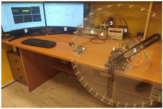
Figure 3. The servo system.

The plant was modelled by Equations (1)–(4) transformed to obtain (5). The angular position $x_1=0$ denotes the lower equilibrium of the arm and the positive direction means the clockwise movement. The load (2) is caused by the gravitation, hence:

$$\overline{L}=\overline{c}\sin x_1,\overline{c}=Mgl,\mathrm{S}\left(x_1,x_2\right)=\sin x_1,$$

(71)

where $M=0.84 \mathrm{kg}$—mass of the arm, $l=0.165 \mathrm{m}$—distance from the gravity center of the arm to the motor’s axis, and $g=9.81 \mathrm{m}/{\mathrm{s}}^2$ is the gravitational acceleration.

The inertia $\overline{m}$ represents the moment of inertia of the arm and the rotor together. The friction was modelled by Equation (3). The nominal parameters ${\overline{m}}_0$, ${\overline{c}}_0, {\overline{b}}_0$, ${\overline{T}}_0$ were guessed from the producer data and from a simple identification experiment and were:

$${\overline{m}}_0=0.0265 {\mathrm{kgm}}^2, {\overline{c}}_0=1.36 \mathrm{Nm}, {\overline{b}}_0=5.9·{10}^{-3} {\mathrm{Nms}/\mathrm{rad}}^2, {\overline{T}}_0=0.029 \mathrm{Nm}$$

(72)

The torque $\tau$ produced by the motor is proportional to the quadrature axis current of the motor $I$ and the nominal torque constant of the motor is $K_{\tau }=0.147\mathrm{Nm}/\mathrm{A}.$ The maximum current of the motor was 19.9 A and corresponded to the maximum torque 2.93 Nm.

The desired motion trajectory $x_{1d}\left(t\right)$ was constructed by connecting the segments presented in Figure 4.

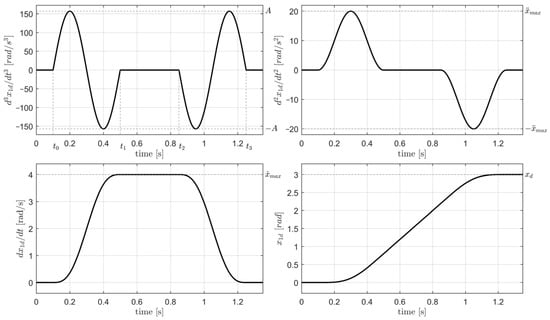
Figure 4. The desired angular position trajectory (a segment) and its derivatives.

From $t_1$ to $t_2$the servo moved with a constant angular velocity. It stopped at the initial position for $t_0$ seconds and stopped again starting from $t_s$ at the final position $x_d$. During the tests several similar segments were connected. The maximum velocity and acceleration were the same for all of them, while the final position $x_d$ changed for each segment.

6.2. Simulations

The drive was modelled with the nominal parameters (72). The simulations aimed to illustrate the influence of the design parameters and characteristic features of the closed-loop system.

6.2.1. CASE 1. All Plant Parameters Were Known, the Unstructured Disturbance Was Zero

In this case the adaptation was not necessary, so the adaptive laws were inactive. The controller used the accurate (rather than adaptive) parameters. The controller gains were selected: $k_1=0.1$, $k_2=0.1$. Initial conditions for the angular position and velocity were: $x_1\left(0\right)=-0.16 \left[rad\right]$, $x_2\left(0\right)=-0.8\left[rad/s\right]$.

First, the system operation without any constraints is demonstrated in Figure 5 and Figure 6. It was achieved by taking $T_1=T_1=Inf$, $r=q=1000$.

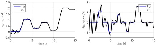
Figure 5. Angular position and velocity compared with the desired values. The constraints are inactive.

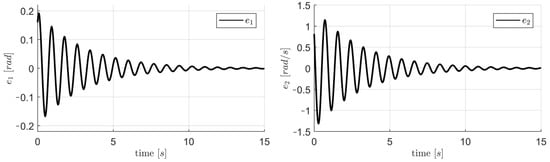
Figure 6. Tracking errors. The constraints are inactive.

Next, for the same desired position trajectory depicted in Figure 5, the case of constant constraints $B_1$ and $B_2$ was considered. As is presented in Figure 7, both errors remained inside the constraints.

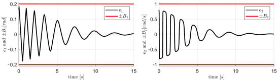
Figure 7. Tracking errors under constant constraints.

Finally, time varying constraints $B_1\left(t\right)$ and $B_2\left(t\right)$ were investigated for several combinations of parameters $T_1$ and $T_2$. The desired trajectory was the same as depicted in Figure 5. In any case the tracking errors were effectively bounded—see Figure 6, Figure 7, Figure 8, Figure 9, Figure 10 and Figure 11. As it is visible from Figure 10, when $T_1\ll T_2$ (fast position constraint in the presence of large velocity bound), the tracking errors oscillated between the constraints rapidly. Such chattering is definitely not recommended in a real system. The initial subinterval of the position and velocity time-history is presented against the background of $x_{1d}\left(t\right)$ and ${\dot{x}}_{1d}\left(t\right)$ together with the constraints taken from the inequality (69).

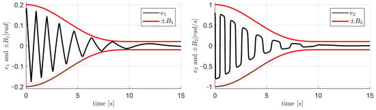
Figure 8. Tracking errors $e_1$, $e_2$ together with the time-varying constraints $B_1$ i $B_2$. Parameters: $r=0.2$, ${\epsilon }_1=0.02$, $q=1$, ${\epsilon }_2=0.1$, $T_1=10 \mathrm{s}$, $T_2=10 \mathrm{s}$.

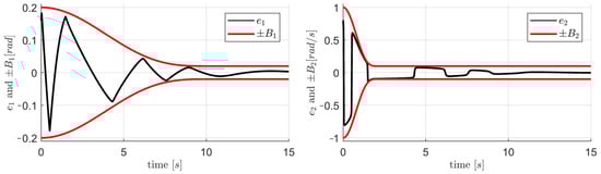
Figure 9. Tracking errors $e_1$, $e_2$ together with the time-varying constraints $B_1$ i $B_2$. Parameters: $r=0.2$, ${\epsilon }_1=0.02$, $q=1$, ${\epsilon }_2=0.1$, $T_1=10 \mathrm{s}$, $T_2=2 \mathrm{s}$.

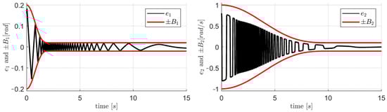
Figure 10. Tracking errors $e_1$, $e_2$ together with the time-varying constraints $B_1$ i $B_2$. Parameters: $r=0.2$, ${\epsilon }_1=0.02$, $q=1$, ${\epsilon }_2=0.1$, $T_1=2 \mathrm{s}$, $T_2=10 \mathrm{s}$.

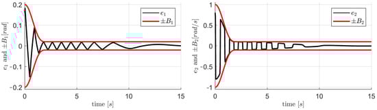
Figure 11. Tracking errors $e_1$, $e_2$ together with the time-varying constraints $B_1$ i $B_2$. Parameters: $r=0.2$, ${\epsilon }_1=0.02$, $q=1$, ${\epsilon }_2=0.1$, $T_1=2 \mathrm{s}$, $T_2=2 \mathrm{s}$.

As the main control aim was to follow a given position trajectory, some difference between $x_2$ and ${\dot{x}}_{1d}$ has to be accepted. The drive should have some “overspeed” to react properly to disturbances and parameter changes (Figure 12).

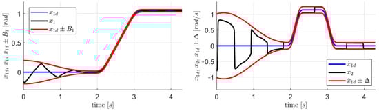
Figure 12. Angular position $x_1$ and velocity $x_2$ together with the desired values and the constraints $\mathsf{\Delta }=\left|{\dot{B}}_1\right|+k_1{B}_1+B_2$, parameters as in the Figure 11.

6.2.2. CASE 2. Constant Parameters Were Unknown, the Unstructured Disturbance Was Absent

In this case the ‘robustifying’ term $-{\widehat{D}}_M\tanh \left(\frac{D_2{\mathrm{A}}_2}{\kappa }\right)$ in the control (48) was not necessary, and neither was the adaptive law for ${\widehat{D}}_M.$It was assumed that no estimates of the values of the system parameters were available; hence, all initial conditions for adaptive parameters were zeros. The selected controller parameters were: $r=0.2$, ${\epsilon }_1=0.02$, $q=1$, ${\epsilon }_2=0.1$ $T_1=T_2=5 \mathrm{s},$ $k_1=k_2=1$, ${\gamma }_m=1$, ${\gamma }_c=10$, ${\gamma }_b=1$, ${\gamma }_T=10$, ${\gamma }_D=0$, and only lower constraints, all equal to zero, were used in the adaptive laws. The desired trajectory was the same as the one depicted in Figure 4. As is demonstrated in Figure 13, all tracking errors remained inside the constraints; moreover, the errors approached zero for $t\to \infty$. The adaptive parameters remained inside the constrained set, according to the projection operators in the adaptive laws. All adaptive parameters approached the real plant parameters. The changes in the adaptive parameters near the constraints were quite rapid, as is typical for adaptive laws using projection, but fortunately, the motor current (proportional to the torque) was far smoother and safely bounded (Figure 14).

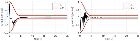
Figure 13. Tracking errors $e_1$, $e_2$ in CASE 2.

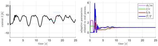
Figure 14. The motor current $I$ and the adaptive parameters related to real plant parameters—CASE 2.

6.2.3. CASE 3. Unstructured Disturbance

It was assumed that the real friction was described by the Stribeck curve [34]:

$$\overline{F}=\overline{b}{x}_2+\overline{T}sign\left(x_2\right)+0.03e^{-10\left|x_2\right|}sign\left(x_2\right)$$

(73)

and the last component $F_{\mathrm{S}}=0.03e^{-10\left|x_2\right|}sign\left(x_2\right)$was neglected during the controller design. The influence of this component on the complete friction curve is explained in Figure 15. As a result, the unmodeled friction $F_{\mathrm{S}}$ generated the unstructured, bounded disturbance $\overline{d}\left(t\right)=0.03e^{-10\left|x_2\left(t\right)\right|}sign\left(x_2\left(\mathrm{t}\right)\right)$.

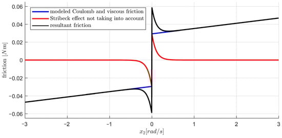
Figure 15. Stribeck curve and its components.

If no remedial measures were taken, i.e., the controller was exactly the same as in CASE 2, the quasi-steady-state tracking error is evidently visible (Figure 16). If the adequate control component together with the adaptive law (61) is introduced with parameters $\kappa =1/100$, ${\gamma }_D=10$, ${\sigma }_D=1$, both tracking errors were substantially reduced (Figure 17).

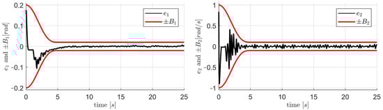
Figure 16. Tracking errors $e_1$, $e_2$—the controller without unstructured disturbance compensation.

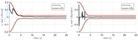
Figure 17. Tracking errors $e_1$, $e_2$—the controller with unstructured disturbance compensation.

6.2.4. CASE 4. System Reaction to an Unanticipated Change of Parameters

The controller was designed assuming that the plant parameters were unknown, but constant. It was demonstrated that the proper operation was achieved even if the adaptive parameters substituting the real ones started from zero initial conditions. Here, the system robustness was tested against the unexpected change of parameters during the motion. The regulator was exactly the same as used in CASE 3.

The mass of the arm was increased by 50% at the 20th second of motion, when the servo operated inside narrow constraints ${\epsilon }_1$, ${\epsilon }_2$. In effect, two model parameters, the moment of inertia $m$ and the load parameter $c$, were changed. It was observed (Figure 18 and Figure 19) that the tracking errors increased, almost reaching the bound (without breaching it), and went back to standard values. Adaptive parameters corresponding to $m$ and the load parameter $c$ moved to the new values, adequate to the change of model parameters. The remaining adaptive parameters also reacted but returned to the previous values. Therefore, it can be concluded that the system is robust against the unexpected change of plant parameters.

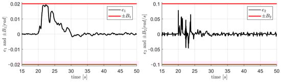
Figure 18. Tracking errors $e_1$, $e_2$ caused by 50% increase in manipulator mass at $t=20 \mathrm{s}$.

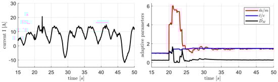
Figure 19. Motor current and selected adaptive parameters changing after a 50% increase in the manipulator mass at $t=20 \mathrm{s}$.

6.2.5. CASE 5. Simulations Including the Hardware

Before implementing the control algorithm in the real system, a series of simulations were carried out in which it was assessed how the real hardware will affect the correct operation of the system. The controller used in CASE 3 and 4 was supplemented with blocs modeling:

• the current control loop, including a fast PI controller, modelled by the transfer function $G_i\left(s\right)=\frac{I_M\left(s\right)}{I_d\left(s\right)}=\frac{1}{{10}^{-4}s+1}$, where $I_M$ denotes the generated motor current and $I_d$ is the desired current: $I_d={\mathrm{sat}}_{19.9} \left(I\right)$, where $I$ is the control command calculated from (48) and ${\mathrm{sat}}_{19.9}$ means $\pm 19.9$ saturation;
• $50 \mathsf{\mu }\mathrm{s}$ sampling of the whole system;
• finite encoder resolution which equals $\frac{2\pi }{2^{13}}~0.0008 \mathrm{rad}~0.045 \mathrm{deg}$;
• differential filter for velocity calculation (Savitzky-Golay Smoothing and Differentiation Filter using 130 samples) [35].

Examples of the effects of the simulations are presented in Figure 20, Figure 21 and Figure 22. The parameters defining the constraints were $R_1=0.3$, ${\epsilon }_1=0.03$, $R_2=2$, ${\epsilon }_2=0.5$ and $T_1=5 \mathrm{s}$, $T_2=5 \mathrm{s}$.

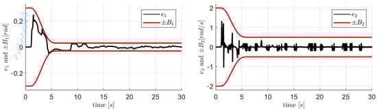
Figure 20. Tracking errors $e_1$, $e_2$.

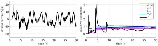
Figure 21. Desired motor current and adaptive parameters.

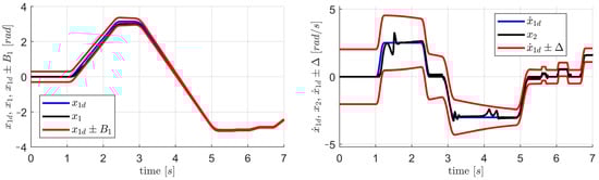
Figure 22. Angular position $x_1$ and velocity $x_2$ together with the desired values and the constraints $\mathsf{\Delta }=\left|{\dot{B}}_1\right|+k_1{B}_1+B_2.$

The simulations were run many times with various:

• constraints;
• adaptation gains;
• controller gains;
• encoder resolutions;
• sizes of the velocity measuring filter;
• inertia of the current control loop.

Due to the limited volume of the paper, not all plots are shown, but the following conclusions may be reported:

• The main factor limiting the system performance is the filter–encoder cooperation. The filter not only introduces a delay in the engine speed measurement path, but it also adds some noise. In the tested case, the noise amplitude was about $0.2 \mathrm{rad}/\mathrm{s}$, which effectively limited the acceptable parameter ${\epsilon }_2$. A reasonable choice is ${\epsilon }_2\ge 0.5 \mathrm{rad}/\mathrm{s}$;
• For the investigated desired motion trajectories, the system was robust against the motor current saturation and the current control time-constant up to $100 \mathsf{\mu }\mathrm{s}$;
• It is recommended that $T_2\le T_1$;
• Too fast an adaptation (high adaptation gain) causes a chattering of the tracking errors inside the constraints;
• The parameters of the hardware used strongly affect the performance of the system. For example, the speed constraint ${\epsilon }_2=0.5 \mathrm{rad}/\mathrm{s}$ is connected to the encoder resolution and noise. The higher resolution of the encoder enables the filtering window to be shortened and the ${\epsilon }_2$ to be reduced several times.

6.3. Real Time, Real Plant Application

The results of the simulations and the numerical experiments were encouraging, so the controller was implemented in a real control hardware presented in Figure 3. Of course, it is impossible to obtain exactly the same results in a real plant as in a simulation. Many of the additional factors, such as the coupling elasticity, nonlinear current–torque characteristics, and unmodelled friction, affect a real plant. However, the results of real plant experiments were similar to the plots presented in Section 6.2.5, where some additional hardware was included into the simulation model.

Although some initial estimations are available, in order to test the worst-case situation, it was assumed that the initial values of all the adaptive parameters were zeros and all lower bounds in the projections were zeros. The controller gains were $k_1=0.1$, $k_2=1$; $\kappa =1/300$.

The examples of plots, collected during three different runs of the servo are presented below.

6.3.1. RUN 1—Fast Motion

The maximum velocity of the desired motion was $\max {\dot{x}}_{1d}=5\mathrm{rad}/\mathrm{s}$. The parameters of the constraints were $r=0.2$, ${\epsilon }_1=0.01$, $q=2$, ${\epsilon }_2=0.5$ and $T_1=5 \mathrm{s}$, $T_2=5 \mathrm{s}$.

Both tracking errors were inside the constraints, although occasionally quite close to them (Figure 23). This resulted in the rapid changes of the adaptive parameters and may have caused higher control values (Figure 24). The servo angular position and the velocity related to the desired values are presented in Figure 25.

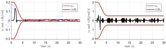
Figure 23. Tracking errors $e_1$, $e_2$.

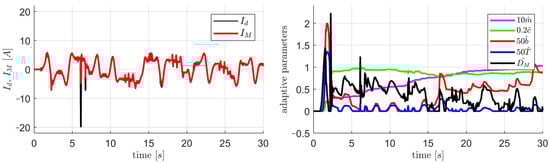
Figure 24. Desired $I_d$ and generated $I_M$ motor current (left). Time-evolution of adaptive parameters (right).

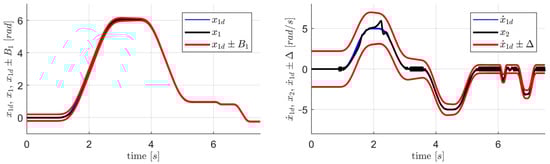
Figure 25. Angular position $x_1$ and velocity $x_2$ together with the desired values and the constraints $\mathsf{\Delta }=\left|{\dot{B}}_1\right|+k_1{B}_1+B_2.$

6.3.2. RUN 2—Moderate Motion

The maximum velocity of the desired motion was $\max {\dot{x}}_{1d}=3\mathrm{rad}/\mathrm{s}$. The parameters of the constraints were $r=0.1$, ${\epsilon }_1=0.03$, $q=2$, ${\epsilon }_2=0.5$ and $T_1=10 \mathrm{s}$, $T_2=5 \mathrm{s}$.

Compared with RUN 1, the motion was slower, and it started closer to the desired position trajectory. Tracking errors were kept far from the constraints, therefore the trajectories of the adaptive parameters were smoother, and the control values were lower (Figure 26 and Figure 27). The servo angular position and the velocity related to the desired values are presented in Figure 28. Obviously, the tracking errors never violated the constraints.

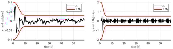
Figure 26. Tracking errors $e_1$, $e_2$.

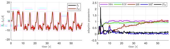
Figure 27. Desired $I_d$ and generated $I_M$ motor current (left). Time-evolution of the adaptive parameters (right).

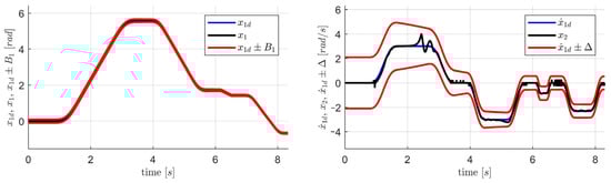
Figure 28. Angular position $x_1$ and velocity $x_2$ together with the desired values and the constraints $\mathsf{\Delta }=\left|{\dot{B}}_1\right|+k_1{B}_1+B_2.$

6.3.3. RUN 3—Slow Motion

The maximum velocity of the desired motion was $\max {\dot{x}}_{1d}=0.5\mathrm{rad}/\mathrm{s}$. The parameters of the constraints were $\mathrm{r}=0.1$, ${\epsilon }_1=0.03$, $q=2$, ${\epsilon }_2=0.5$ and $T_1=5\mathrm{s}$, $T_2=5\mathrm{s}$.

The plots present the quasi-steady state operation. The angular tracking error was very small: $\left|e_1\right|\approx 0.004 \mathrm{rad}$ which is close to the resolution of the encoder (Figure 29). Some difficulties in the measurement of low velocity are visible (Figure 30).

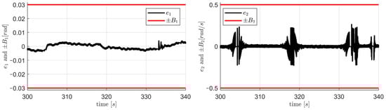
Figure 29. Tracking errors $e_1$, $e_2$

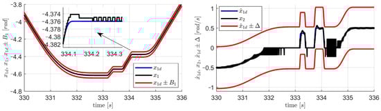
Figure 30. Angular position $x_1$ and velocity $x_2$ together with the desired values and the constraints $\mathsf{\Delta }=\left|{\dot{B}}_1\right|+k_1{B}_1+B_2.$

7. Conclusions

The main advantage and the major novelty of the proposed design method are that a designer can impose a settling time and a tracking accuracy explicitly. Moreover, it is easy to impose inviolable constraints on both state variables—position and velocity. All the attractive features of the closed-loop system were robust against unknown parameters and unstructured perturbations, which may include any disturbances, modelling errors, or unrecognized dynamics.

Special, time-varying barrier Lyapunov functions of both tracking errors resulted in practical, finite-time tracking and the preservation of the strict position and velocity constraints. An adaptive backstepping controller with a robust component assured the stability of the system. Structured uncertainties and unstructured disturbances were used in the model and during the adaptive control design. This made it possible:

• to refer to real, physical servo parameters and include any unmodelled factors at the same time;
• to model the real drive sufficiently accurately;
• to propose reasonable initial conditions of adaptive parameters and realistic constraints for projection operators used in adaptive laws;
• to obtain a robust closed-loop system;
• to minimize the control effort.

The presented derivation was based on a simple, second-order servo model. It may be considered a simplification, but the presented experiments have proven that it is quite justified. Additionally, the use of such a model made it possible to consider servos with different sources of propulsion. The proposed design technique can be generalized to include a specific, dynamic motor model. In this case, additional, subsequent backstepping loops require the application of linear filters to obtain derivatives of the stabilizing functions (virtual controls) [33]. This technique, also called dynamic surface control (DSC) [36] is used to avoid the explosion of complexity, which is typical for a standard adaptive backstepping [33].

The paper presents a complete engineering procedure, from the controller design, the proof of stability, the rules of the controller tuning, through numerous simulations, up to real drive experiments. It is, therefore, demonstrated that the proposed approach is practically applicable. The attractive features of the servo and the control quality are not diminished even if severe unmodelled factors, such as additional friction, cogging torque, current controller inertia, finite encoder resolution, coupling elasticity, imprecise velocity measurement, and inaccurate control input generation affect the actual system.

Apart from the experiments presented here, the proposed control design was compared with other methods taking state constraints into account, especially described in [13,14], applied for a few servos (rotational as well as linear). It must be stressed that the approach presented here is the only one that allows the imposition of a settling time and a tracking accuracy explicitly. Each approach requires proper tuning, and generally, it is possible to obtain satisfactory results using the procedures presented in [13,14] as well, but the simplicity and the directness of the approach described here is the obvious advantage. All the comparisons also demonstrated that the presented technique overcomes standard PI controllers where the state constraints are achieved by proper parameter tuning and control saturation.

References

- Hasan, M.d.M.; Khan, M.d.R.; Noman, A.T.; Rashid, H.; Ahmed, N.; Reza, S.M.T. Design and Implementation of a Microcontroller Based Low Cost Computer Numerical Control (CNC) Plotter using Motor Driver Controller. In Proceedings of the 2019 International Conference on Electrical, Computer and Communication Engineering (ECCE), Cox’sBazar, Bangladesh, 7–9 February 2019; pp. 1–5. [Google Scholar]
- Yang, X.; Ge, S.S.; He, W. Dynamic modelling and adaptive robust tracking control of a space robot with two-link flexible manipulators under unknown disturbances. Int. J. Control 2017, 91, 969–988. [Google Scholar] [CrossRef]
- Yang, X.; Zheng, X.; Chen, Y. Position Tracking Control Law for an Electro-Hydraulic Servo System Based on Backstepping and Extended Differentiator. IEEE/ASME Trans. Mechatron. 2017, 23, 132–140. [Google Scholar] [CrossRef]
- Wei, X.-L.; Wang, J.; Yang, Z.-X. Robust Smooth-Trajectory Control of Nonlinear Servo Systems Based on Neural Networks. IEEE Trans. Ind. Electron. 2007, 54, 208–217. [Google Scholar] [CrossRef]
- Wu, J.; Zhang, J.; Nie, B.; Liu, Y.; He, X. Adaptive Control of PMSM Servo System for Steering-by-Wire System With Disturbances Observation. In IEEE Transactions on Transportation Electrification; IEEE: Piscataway, NJ, USA, 2021; p. 1. [Google Scholar] [CrossRef]
- Fu, D.; Zhao, X.; Zhu, J. A Novel Robust Super-Twisting Nonsingular Terminal Sliding Mode Controller for Permanent Magnet Linear Synchronous Motors. IEEE Trans. Power Electron. 2021, 37, 2936–2945. [Google Scholar] [CrossRef]
- Wang, B.; Liu, C.; Chen, S.; Dong, S.; Hu, J. Data-Driven Digital Direct Position Servo Control by Neural Network With Implicit Optimal Control Law Learned From Discrete Optimal Position Tracking Data. IEEE Access 2019, 7, 126962–126972. [Google Scholar] [CrossRef]
- Ren, H.-P.; Fan, J.-T.; Kaynak, O. Optimal Design of a Fractional-Order Proportional-Integer-Differential Controller for a Pneumatic Position Servo System. IEEE Trans. Ind. Electron. 2018, 66, 6220–6229. [Google Scholar] [CrossRef]
- Chen, Q.; Yu, X.; Sun, M.; Wu, C.; Fu, Z. Adaptive Repetitive Learning Control of PMSM Servo Systems with Bounded Nonparametric Uncertainties: Theory and Experiments. IEEE Trans. Ind. Electron. 2020, 68, 8626–8635. [Google Scholar] [CrossRef]
- Liu, M.; Chan, K.W.; Hu, J.; Xu, W.; Rodriguez, J. Model Predictive Direct Speed Control With Torque Oscillation Reduction for PMSM Drives. IEEE Trans. Ind. Informat. 2019, 15, 4944–4956. [Google Scholar] [CrossRef]
- Liu, Z.; Zhao, Y. Robust Perturbation Observer-based Finite Control Set Model Predictive Current Control for SPMSM Considering Parameter Mismatch. Energies 2019, 12, 3711. [Google Scholar] [CrossRef] [Green Version]
- Tarczewski, T.; Skiwski, M.; Niewiara, L.J.; Grzesiak, L.M. High-performance PMSM servo-drive with constrained state feedback position controller. Bull. Pol. Acad. Sci. Tech. Sci. 2018, 66, 49–58. [Google Scholar]
- Kabziński, J.; Mosiołek, P. Adaptive, nonlinear state transformation-based control of motion in presence of hard constraints. Bull. Pol. Acad. Sci. Tech. Sci. 2020, 68, 963–971. [Google Scholar] [CrossRef]
- Kabziński, J.; Mosiołek, P. Motion Control with Hard Constraints—Adaptive Controller with Nonlinear Integration. In Advances in Intelligent Systems and Computing; Springer: Singapore, 2020; pp. 449–461. [Google Scholar]
- Doria-Cerezo, A.; Acosta, J.; Castano, A.; Fossas, E. Nonlinear state-constrained control. Application to the dynamic positioning of ships. In Proceedings of the 2014 IEEE Conference on Control Applications (CCA), Juan Les Antibes, France, 8–10 October 2014; pp. 911–916. [Google Scholar]
- Liu, N.; Shao, X.; Yang, W. Integral Barrier Lyapunov Function Based Saturated Dynamic Surface Control for Vision-Based Quadrotors via Back-Stepping. IEEE Access 2018, 6, 63292–63304. [Google Scholar] [CrossRef]
- Liu, Y.; Yu, J.; Yu, H.; Lin, C.; Zhao, L. Barrier Lyapunov Functions-Based Adaptive Neural Control for Permanent Magnet Synchronous Motors With Full-State Constraints. IEEE Access 2017, 5, 10382–10389. [Google Scholar] [CrossRef]
- Tang, L.; Chen, A.; Li, D. Time-Varying Tan-Type Barrier Lyapunov Function-Based Adaptive Fuzzy Control for Switched Systems With Unknown Dead Zone. IEEE Access 2019, 7, 110928–110935. [Google Scholar] [CrossRef]
- Yuan, X.; Chen, B.; Lin, C. Prescribed Finite-Time Adaptive Neural Tracking Control for Nonlinear State-Constrained Systems: Barrier Function Approach. In IEEE Transactions on Neural Networks and Learning Systems; IEEE: Piscataway, NJ, USA, June 2021; pp. 1–10. [Google Scholar] [CrossRef]
- Igarashi, M.; Tezuka, I.; Nakamura, H. Time-varying Control Barrier Function and Its Application to Environment-Adaptive Human Assist Control. IFAC-PapersOnLine 2019, 52, 735–740. [Google Scholar] [CrossRef]
- Wang, F.; Chen, B.; Liu, X.; Lin, C. Finite-Time Adaptive Fuzzy Tracking Control Design for Nonlinear Systems. IEEE Trans. Fuzzy Syst. 2018, 26, 1207–1216. [Google Scholar] [CrossRef]
- Wang, F.; Lai, G. Fixed-time control design for nonlinear uncertain systems via adaptive method. Syst. Control. Lett. 2020, 140, 104704. [Google Scholar] [CrossRef]
- Xia, J.; Zhang, J.; Sun, W.; Zhang, B.; Wang, Z. Finite-Time Adaptive Fuzzy Control for Nonlinear Systems With Full State Constraints. IEEE Trans. Syst. Man, Cybern. Syst. 2019, 49, 1541–1548. [Google Scholar] [CrossRef]
- Wang, C.; Wu, Y. Finite-time tracking control for strict-feedback nonlinear systems with full state constraints. Int. J. Control. 2019, 92, 1426–1433. [Google Scholar] [CrossRef]
- Yang, H.; Ye, D. Adaptive Fuzzy Nonsingular Fixed-Time Control for Nonstrict-Feedback Constrained Nonlinear Multiagent Systems With Input Saturation. IEEE Trans. Fuzzy Syst. 2021, 29, 3142–3153. [Google Scholar] [CrossRef]
- Sun, J.; Yi, J.; Pu, Z. Fixed-Time Adaptive Fuzzy Control for Uncertain Nonstrict-Feedback Systems with Time-Varying Constraints and Input Saturations. In IEEE Transactions on Fuzzy Systems; IEEE: Piscataway, NJ, USA, 18 January 2021; p. 1. [Google Scholar] [CrossRef]
- Ilchmann, A.; Schuster, H. PI-Funnel Control for Two Mass Systems. IEEE Trans. Autom. Control 2009, 54, 918–923. [Google Scholar] [CrossRef] [Green Version]
- Ilchmann, A.; Ryan, E.P.; Townsend, P. Tracking control with prescribed transient behaviour for systems of known relative degree. Syst. Control Lett. 2006, 55, 396–406. [Google Scholar] [CrossRef] [Green Version]
- Wang, S.; Yu, H.; Yu, J.; Gao, X. Adaptive Neural Funnel Control for Nonlinear Two-Inertia Servo Mechanisms With Backlash. IEEE Access 2019, 7, 33338–33345. [Google Scholar] [CrossRef]
- Berger, T.; Reis, T. Funnel Control Via Funnel Precompensator for Minimum Phase Systems With Relative Degree Two. IEEE Trans. Autom. Control 2018, 63, 2264–2271. [Google Scholar] [CrossRef]
- Cheng, Y.; Ren, X. Neural-Network-Based Adaptive Funnel Control for Strict-Feedback Systems with Tracking Error and State Constraints. In Proceedings of the 2021 IEEE 10th Data Driven Control and Learning Systems Conference (DDCLS), Suzhou, China, 14–16 May 2021; pp. 415–420. [Google Scholar]
- Ioannou, P.; Baldi, S. Robust Adaptive Control; Dover Publications: Mineola, NY, USA, 2010. [Google Scholar]
- Kabziński, J.; Mosiołek, P. Projektowanie Nieliniowych Układów Sterowania (Nonlinear Control Design), I; PWN SA: Warszawa, Poland, 2018. [Google Scholar]
- Pennestrì, E.; Rossi, V.; Salvini, P.; Valentini, P.P. Review and comparison of dry friction force models. Nonlinear Dyn. 2016, 83, 1785–1801. [Google Scholar] [CrossRef]
- Luo, J. Savitzky-Golay Smoothing and Differentiation Filter. In MATLAB Central File Exchange; 2021; Available online: https://www.mathworks.com/matlabcentral/fileexchange/4038-savitzky-golay-smoothing-and-differentiation-filter (accessed on 10 December 2021).
- Li, T.; Feng, G.; Zou, Z. DSC-backstepping based robust adaptive fuzzy control for a class of strict-feedback nonlinear systems. In Proceedings of the 2008 IEEE International Conference on Fuzzy Systems (IEEE World Congress on Computational Intelligence), Hong Kong, China, 1–6 June 2008; pp. 1274–1281. [Google Scholar]
Publisher’s Note: MDPI stays neutral with regard to jurisdictional claims in published maps and institutional affiliations. |
© 2022 by the authors. Licensee MDPI, Basel, Switzerland. This article is an open access article distributed under the terms and conditions of the Creative Commons Attribution (CC BY) license (https://creativecommons.org/licenses/by/4.0/).