Combustion Modeling Approach for the Optimization of a Temperature Controlled Reactivity Compression Ignition Engine Fueled with Iso-Octane

Abstract

In this study, an innovative Low Temperature Combustion (LTC) system named Temperature Controlled Reactivity Compression Ignition (TCRCI) is presented, and a numerical optimization of the hardware and the operating parameters is proposed. The studied combustion system aims to reduce the complexity of the Reaction Controlled Compression Ignition engine (RCCI), replacing the direct injection of high reactivity fuel with a heated injection of low reactivity fuel. The combustion system at the actual state of development is presented, and its characteristics are discussed. Hence, it is clear that the performances are highly limited by the actual diesel-derived hardware, and a dedicated model must be designed to progress in the development of this technology. A Computational Fluid Dynamics (CFD) model suitable for the simulation of this type of combustion is proposed, and it is validated with the available experimental operating conditions. The Particle Swarm Optimization (PSO) algorithm was integrated with the Computational Fluid Dynamic (CFD) software to optimize the engine combustion system by means of computational simulation. The operating condition considered has a relatively high load with a fixed fuel mass and compression ratio. The parameters to optimize are the piston bowl geometry, injection parameters and the boosting pressure. The achieved system configuration is characterized by a wider piston bowl and injection angle, and it is able to increase the net efficiency of 3% and to significantly reduce CO emissions from 0.407 to 0.136 mg.

1. Introduction

Currently, the research and development of internal combustion engines is moving towards more efficient systems that are cleaner and able to fulfill the zero emissions targets of recent legislation. Different innovative Low Temperature Combustion (LTC) strategies based on premixed combustion have been investigated to overcome the limits of Compression Ignition (CI) engines in terms of pollutant emissions and efficiency. These combustion concepts are characterized by an ignition delay that guarantees an adequate mixing time. Thus, rich regions are reduced and soot formation is inhibited, while the lower combustion temperatures result in $N{O}_x$ reduction due to the high activation energy of thermal $NO$ formation reactions [1].

The first LTC technology studied is known as Homogeneous Charge Compression Ignition (HCCI), where the injection event is set to guarantee an almost lean and homogeneous mixture at the start of the combustion. The ignition is thus chemically driven: it occurs spontaneously when the charge reaches the thermodynamic conditions necessary to auto-ignite [2]. The drawbacks of this technology are the large Pressure Rise Rate (PRR), the tendency to show knock-like combustion increasing the equivalence ratio and the large combustion sensitivity to environment conditions, especially the air/fuel mixture temperature.

An alternative solution developed to overcome the limits of HCCI is Reaction Controlled Compression Ignition (RCCI) [3]. This type of engine operates with two fuels characterized by different reactivity. A low reactivity fuel, typically gasoline, is port injected, a second high reactivity fuel, typically diesel, is directly injected close to the Top Dead Center (TDC). The high reactivity fuel reacts with low-temperature reactions, releasing enough energy to ignite the homogeneous premixed charge. This two-stage ignition helps to increase the combustion duration and to reduce the peak of the Heat Release Rate (HRR) with respect to HCCI combustion. Unfortunately, this technology requires two different fuels and hence two supply systems, increasing the cost and the complexity of the overall system.

A new technology named TCRCI has been proposed to decrease the complexity of RCCI. It is characterized by the use of a port and a heated direct injection to create a warm and richer region in the lean and homogeneous premixed charge. The basic idea behind this concept is that the reactivity increment, due to the fuel heating, should mimic the effect of the use of a more reactive direct injected fuel in RCCI, stabilizing the combustion. The ignition delay is reduced especially for the decrease of the physical delay [4], particularly in the case of super-critical injection where the fuel is already in a vapor state at the exit of the injector holes. When the injection temperature is below the critical point, the fuel evaporation can take place under standard or flash boiling conditions. Supercritical injectors can be used to avoid high-pressure injectors. This technology can also potentially use the directly injected fuel temperature as a control parameter. A previous comparison between RCCI and TCRCI (with sub-critical direct injection) has been made by F. Gazzola [5]. He has proved that these technologies are characterized by a comparable efficiency and auto-ignition phasing.

So far, this technology has been developed in a modified diesel combustion chamber, since a compression ratio close to the CI engine is necessary to achieve a spontaneous ignition. The hardware of the experimental engine is optimized for a diffusive combustion, which is far from the characteristics required by the premixed combustion that characterizes the LTC technologies. This existing combustion chamber is therefore expected to limit the performance of the studied combustion concept. Then, an optimized hardware must be conceived to advance the design of this technology. Therefore, the goal of this paper is to propose a numerical methodology to understand the requirements of this concept and guide the design of the new hardware. The study is divided into three specific objectives:

• The first goal of this study is the understanding of the combustion evolution in this innovative technology. Then, the influence of the fuel properties and direct injection temperature on the combustion system is analyzed. In particular, the level of influence of the cylinder temperature with respect to the fuel temperature and the effect of the fuel temperature on the ignition delay must be understood. For these purposes, a 0D methodology has been developed to gain a general understanding of the parameters of interest.
• The second objective is to develop a 3D model to capture the characteristics that are impossible to obtain in the 0D analysis, such as the influence of distribution between direct and port injected fuel. For this, a 3D CFD model is presented and validated with experimental pressure and heat release rate traces at three different operating conditions.
• The third objective is to couple the PSO algorithm with a 3D-CFD software to obtain an optimized combustion system for TCRCI. The optimization process is divided into two stages: the first part is focused on the evaluation of the hardware and the temperature of the mixture at intake valve closing (IVC), while the second optimization regards the hardware (piston geometry and Spray Angle (SA)), the air management and the injection parameters. It has been chosen to introduce all these parameters since the variation of the operating conditions allow us to discover some hardware configurations that could be problematic with the original engine settings. The optimization target is the efficiency, restricted by the peak of pressure rate and in-cylinder pressure. A limit on the pressure increase rate is imposed since a faster combustion brings the cycle closer to the ideal Otto rate, increasing the thermodynamic efficiency.

2. TCRCI Technology

TCRCI is a single fuel LTC combustion mode operating with gasoline-like fuels, where the reactivity stratification is enhanced by heating the direct-injected fuel, in contrast to RCCI mode, which requires two different fuels. The GDI direct injector is equipped with a resistance that is able to heat the fuel up to 500 °C. The hardware used to increase the temperature of the fuel for the direct injection consists of a heater that is located immediately before the injector. It is a heating hose, formed by a pipe with an electric heater inside. The system has two thermocouples: one inside the heating pipe, and the second added between the heater and the GDI injector for further temperature control. Depending on the fuel distribution and injection temperature, the expected combustion behavior is between stratified HCCI and RCCI combustion [3]. The goal of the heated fuel is to trigger the combustion of the premixed charge; hence, the portion of direct injected fuel is about 20–50% of the total fuel mass. This fuel distribution level is common between the various LTC technologies.

Under specific operational conditions, the injected fuel can exceed the critical temperature. This condition could enhance the reactivity stratification by preventing fuel evaporation from cooling the charge temperature. An increase in combustion stratification in comparison with other single fuel LTC technologies slows down the combustion, and it allows the maximum engine load to be increased. On the contrary, increased reactivity can produce efficient combustion with limited polluting emissions for a lean mixture.

The theoretical advantages of this technology with respect to RCCI are as follows:

• A marked simplification of the fuel supply system.
• A lower injection pressure, with values typical of GDI injectors (300 bar).
• The possibility to use 98 RON fuels without problem.

On the other hand, the reactivity stratification with a comparable fuel distribution is expected to be smaller with respect to TCRCI.

The new challenges associated with this technology relate to direct injection temperature monitoring and control.

TCRCI Technology Development

The research into this technology has been experimentally performed on a 3+1 engine (retrofit of a commercial diesel engine). One cylinder has been disconnected from the original diesel injection system and the common intake manifold. Then, it has been equipped with a single manifold with a gasoline port injector and an experimental heated direct injector; it is therefore able to operate both with an HCCI and TCRCI mode. The other cylinders operate with the original diesel combustion to stabilize the engine behavior. A Horiba exhaust gas analyzer has been connected to the exhaust pipe to measure polluting emissions and the equivalence ratio. Figure 1 shows a simplified scheme of the described configuration, while

Table 1. Test bench engine specifications. Reference crank angle (0 CAD) is Top Dead Center with closed valves.

Bore [mm]	83
Stroke [mm]	90.4
IVC [CAD]	−153
EVO [CAD]	124
Injector hole number	6
Nozzle Holes Diameter [$\mathsf{\mu }$m]	219
Spray angle [°]	120

summarizes the main engine data.

Different operating conditions and engine loads have been tested in the described hardware to assess the potential of this new combustion strategy. Figure 2 shows a summary of the experimental campaign in an efficiency load map. At the current state of development, this technology is able to achieve a gross indicated efficiency above $40\%$ for a range of engine loads between 4 and 14 bar. This range is close to that achievable with RCCI technology [3].

The $N{O}_x$ emissions are well below 25 ppm for the large majority of the points. This level is much lower than a conventional diesel engine [6].

3. Methodology

This work is based on two different types of numerical analysis. Firstly, a basic 0D analysis based on the concept of the mixing line is carried out to achieve some general conclusions on the combustion characteristics and the influence of the fuel temperature on the evolution of the in-cylinder properties. This type of analysis is also useful to define the fuel properties that could improve this specific technology. It is followed by CFD simulations to extend the conclusions drawn with the 0D model and to capture the influence of the injection parameters on the fuel stratification and the combustion evolution. Finally, the CFD model is coupled to the evolutionary algorithm and processing tools used for the optimization.

3.1. Mixing Line

The goal of this preliminary study is to model, in the simplest way possible, the evolution of the fuel jet temperature during the mixing process, in order to understand its influence on the Ignition Delay (ID) of the mixture. In this way, it is possible to determine the parameters that have more influence on the combustion evolution. This analysis is performed using Cantera, an open-source suite of tools for problems involving chemical kinetics, thermodynamics and transport processes, and the adopted model is described here. The temperature evolution as a consequence of the mixing process is calculated from the first law of thermodynamics:

$$m_f·C_{p,f}\left(T\right)·\left(T_f-T\right)=m_{air}·C_{p,air}·\left(T_{air}-T\right)$$

(1)

where $T_f$ is the fuel temperature at the exit of the injector hole, $T_{air}$ is the average in-cylinder temperature, and $C_p$ is the specific heat. The fuel is always considered in the gaseous state; thus, the heat of vaporization is never considered in the model, as it is suitable only for supercritical injection.

The fuel and air mass are related by the equivalence ratio:

$$m_{air}=m_f·{\left(m_{air}/m_f\right)}_{stoic}/\varphi$$

(2)

The total mass is set from the state equation for ideal gas, considering the in-cylinder thermodynamic conditions at the end of the direct injection. The local temperature equation is simply a function of the equivalence ratio ($T=f\left(\varphi \right)$), and it models the temperature evolution in an ideal instantaneous spray where the cells do not interact between each other; the diffusion phenomena are therefore neglected. For each point defined in the $T-\varphi$ space, a constant pressure reactor equation is used to set the local ignition delay. This step requires the use of a chemical–kinetic mechanism. For this purpose, the ID is defined as the time when the global normalized progress variable reaches a value equal to 0.1 [7]. 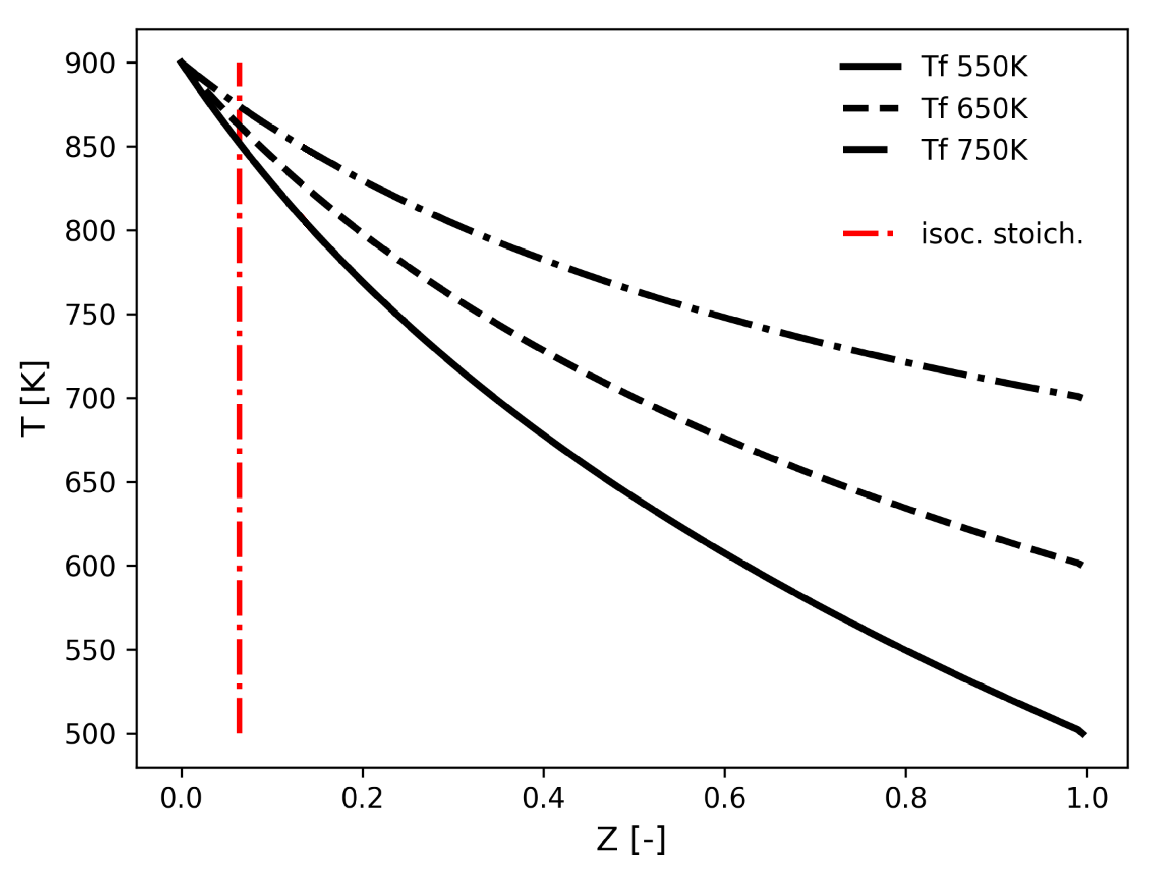Finally, a relation such as $ID=f\left(T\right(\varphi \left)\right)$ is obtained. This analysis aims to model, in the simplest possible way, an abstract injection by defining the temperature stratification and the resultant stratification of ID. It is firstly necessary to set the temperature evolution in the range from Z = 0—a condition not affected by the injection—to Z = 1—the condition at the exit of the nozzle hole. It is important to notice that in real conditions, at the start of the DI, the port injected fuel is already homogeneously mixed in the charge. The presence of this fuel has been neglected since it is a constant and does not affect the trend of the evolution. Furthermore, this analysis is qualitative and not quantitative; therefore, this omission does not influence the general conclusion achieved. The first relevant consideration is that, to have a significant fuel stratification, the injection timing for these type of LTC strategies is close to the TDC (between −40 and −20 CAD), and thus the in-cylinder temperature is close to 800/900 K. Moreover, the fuel still cools down the charge temperature in the vast majority of the possible operating conditions. Figure 3 represents the temperature evolution of the mixing line considering a charge temperature equal to 900 K and a sweep of fuel temperature between 550 and 750 K; different properties can be discussed here. At first, the range of mixture fractions interested by the combustion is characterized by a small fuel mass. Therefore, the variation of the charge temperature is much more influential with respect to the fuel temperature. The sensibility of the LTC technologies to variation of the charge conditions is well known, and it is responsible for their limited control.

Once the temperature evolution has been set, it is possible, for each temperature-equivalence ratio point, to perform a constant pressure reactor calculation to define the corresponding ignition delay. It is known that one of the most important fuel properties for stratified LTC technologies is the so-called phi sensitivity [8], defined as follows:

$$Norm\left({\varphi }_{sensitivity}\right)=-\frac{1}{ID}\frac{d\left(ID\right)}{d\varphi }$$

(3)

This property reflects the effectiveness of the stratification, since an increase of the equivalence ratio follows a decrease of the ignition delay. This property promotes a slower combustion, avoids a sudden pressure increase and allows the maximum load achievable by the engine to be increased, decreasing the knock tendency. Note that it is normalized to properly compare conditions that have very different ignition delays, and it has been chosen to use the negative sign to use a positive value for correct behavior.

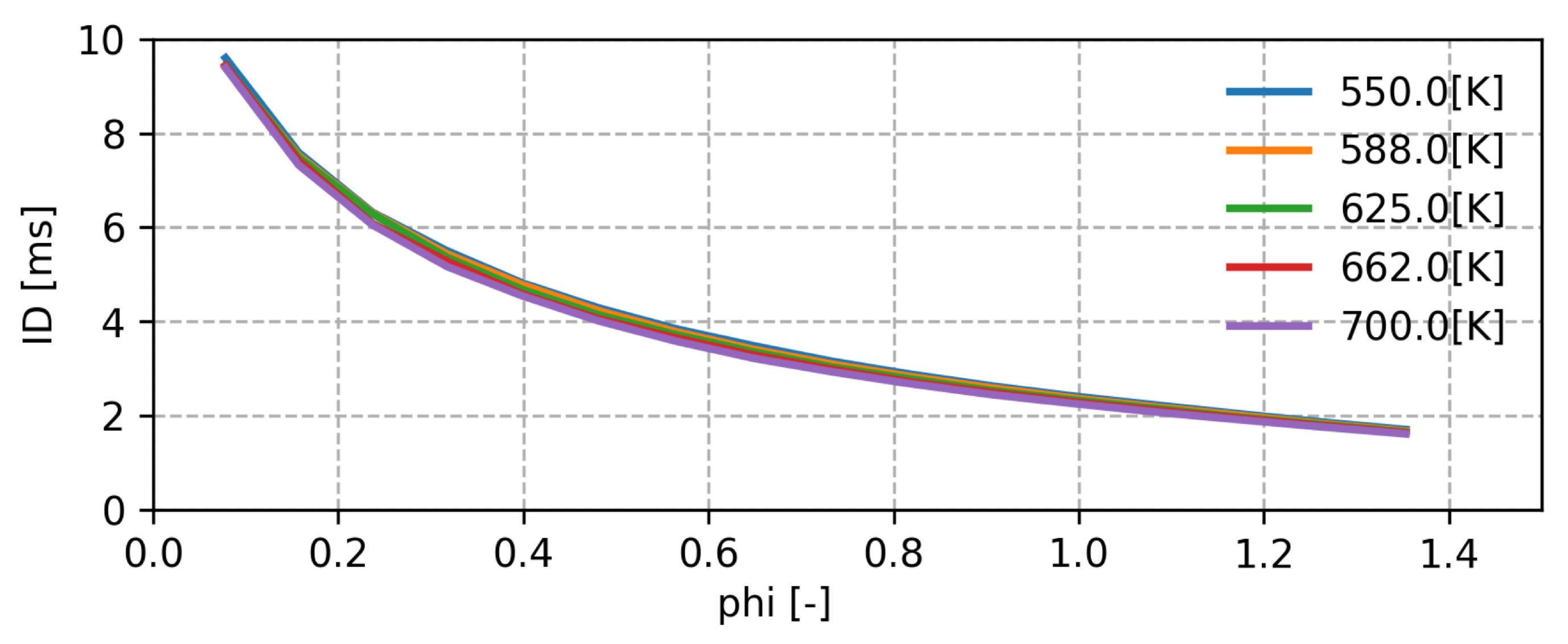
Figure 4 depicts the behavior of iso-octane under the following conditions: the in-cylinder temperature and pressure are 900 K and 65 bar, while the fuel ranges from 550 to 700 K. These values are representative of the thermodynamic state of the medium load case of the engine (defined as case b in the further section of validation) at −15 CAD. They have been chosen to be relatively close to the start of the main combustion to guarantee a good fuel reactivity. Since these conditions come after the end of the injection, the difference between the fuel and the in-cylinder temperature is higher, and thus the effect of the fuel temperature is probably quite over-estimated. However, this issue is limited since the diffusion of the direct injected fuel is not instantaneous, and the mixing continues well after the injection. The first important result is that iso-octane shows a negative phi sensitivity in the whole range of interest. It is also interesting that the ID of this fuel is almost not influenced by the fuel temperature—this characteristic is probably the result of the high stoichiometric air–fuel ratio of hydrocarbons.

It must be noted that this analysis was carried out in gaseous conditions. The total ignition delay of a supercritical injection is, however, always smaller than a cold injection, since the fuel evaporation is much faster. The results of the analysis suggest that, for iso-octane, the benefits resulting from a further increase of the injection temperature above the supercritical one are minimum. These results are useful for the determination of the initial conditions for CFD simulations and to have an idea of the expected combustion evolution.

3.2. CFD

The CFD analysis is performed in LibICE, a set of applications and libraries for Internal Combustion Engine (ICE) simulations, with pre and post-processing implemented in the OpenFOAM framework, developed by the Politecnico di Milano–ICE group [9,10,11,12]. It provides tools and solvers to model physical and chemical phenomena, such as liquid spray dynamics and evolution, combustion processes and exhaust gases after treatment. The simulations performed here are defined as a closed cycle. They range from Inlet Valve Closing (IVC) to Exhaust Valve Opening (EVO) and allow the combustion characteristics to be captured without modeling the air exchange process; thus, the required computational time is significantly reduced. The models used for combustion, turbulence and injection are described below.

3.2.1. Combustion Model

This technology is based on a stratified spontaneous ignition premixed combustion. The engine operates with commercial pump gasoline, while the simulations are performed using iso-octane. The combustion model used is based on the flamelet approach, and it is the well-known Tabulated Well Mixed (TWM) [13]. The main advantage of the flamelet approach is the decoupling of the flame structure from the flow dynamics [14]. This property is obtained via the introduction of the conserved scalar: mixture fraction Z, commonly defined based on the elements conservation. In the well-mixed model, each computational cell of the reactive mixture is treated as a closed homogeneous system, neglecting turbulence–chemistry interaction for the local flow conditions. Furthermore, this model allows the chemical computation to be decoupled from the CFD simulations, since the reaction equations are previously solved and the relevant quantities stored in a table as a function of the state variables of the system and the combustion progress variable. The adopted reduced chemical kinetic mechanism is a gasoline surrogate reduced mechanism developed by the Creck Group [15].

3.2.2. Injection Model

The injection phenomenon in this particular technology is challenging to model and investigate since the physics and the modeling techniques change with the passage from liquid to super-critical injection. Commercial pump gasoline is a complex, multi-component fluid with a boiling point that ranges from 533 to 618 K [16], while the reference fuel used in the simulation (iso-octane) has a critical point equal to 544 K and 25.6 bar [17]. The super-critical injection of gasoline has not been deeply investigated up to now; however, a larger bibliography is present in the aerospace field for different liquids such as LN${}_2$. It has been experimentally proved that super-critical injection shows similar characteristics with respect to turbulent gas jets when the injection pressure is above the critical pressure [18], as in the analyzed case. Conversely, the behavior is close to liquid jets for sub-critical pressure. An internally developed virtual gaseous injection model is therefore used. This model directly injects inside the cylinder gaseous fuel excluding from the computational domain the injector nozzle. This allows to avoid to model the complex phenomena that happens inside the injector, like the phase change from liquid to super-critical. The model approach is based on the work of Baratta et al. [19,20].

A set of source cells in correspondence of the injector hole is defined to directly introduce the gaseous fuel inside the cylinder domain based on an imposed injection profile. The complex thermo-physical phenomena that occur in the injector pipe are also neglected. For the injector cell set, an additional source term proportional to the mass flow rate is added for the finite-volume equations of density, turbulent kinetic energy, velocity and mixture fraction to take into account the gaseous injection:

$$S_{\mathrm{\Phi }}=\dot{m}·\mathrm{\Phi }$$

(4)

where $\dot{m}$ is the injection mass flow rate and $\mathrm{\Phi }$ is a generic transported property [19,20]. The injected fuel is considered as an ideal gas. This choice has been made since this approximation has a small influence on the mixture characteristics far from the injector, where the combustion reactions take place. A better description of the near nozzle processes will be a matter of investigation in a future work. So far, the adopted approach seems to provide a good estimation of experimental data.

3.2.3. Turbulence Model

Turbulence plays an important role in the combustion process of ICE. The model used in this work is the well known $k-\epsilon$ [21]. It is the most common turbulence model and can provide a stable and accurate description of the effects of turbulence on the average fluid motion, since it solves RANS equations.

3.2.4. Mesh Generator

The mesh is fully automatically computed by Python-based software developed by the Politecnico di Milano–ICE group that is able to provide a spray-oriented and fully hexahedral mesh. The procedure is based on a angular extrusion from a base 2D mesh composed of three regions: (1) the spray region, which is the region where the spray mainly evolves; (2) the layer region, which is the one involved in the layer addition process in the moving mesh; and (3) the piston region [10]. The regions are automatically computed based on the piston geometry, the spray angle and the injector hole position. This meshing procedure relies on the definition of some constants, which allows the meshing to be tuned to different geometries. However, when the piston geometry and the spray angle change in a wide range, it is difficult to achieve a good mesh in the extremes of the domain.

Table 2. CFD models specifications.

Injection	Blob Injector
Break-up	KH-RT
Collision	off
Evaporation	Adachi Flash Boiling
Turbulence	$k-ϵ$ RANS
Wall heat transfer	Angelberger
Combustion	TWM

summarizes the information regarding the models used.

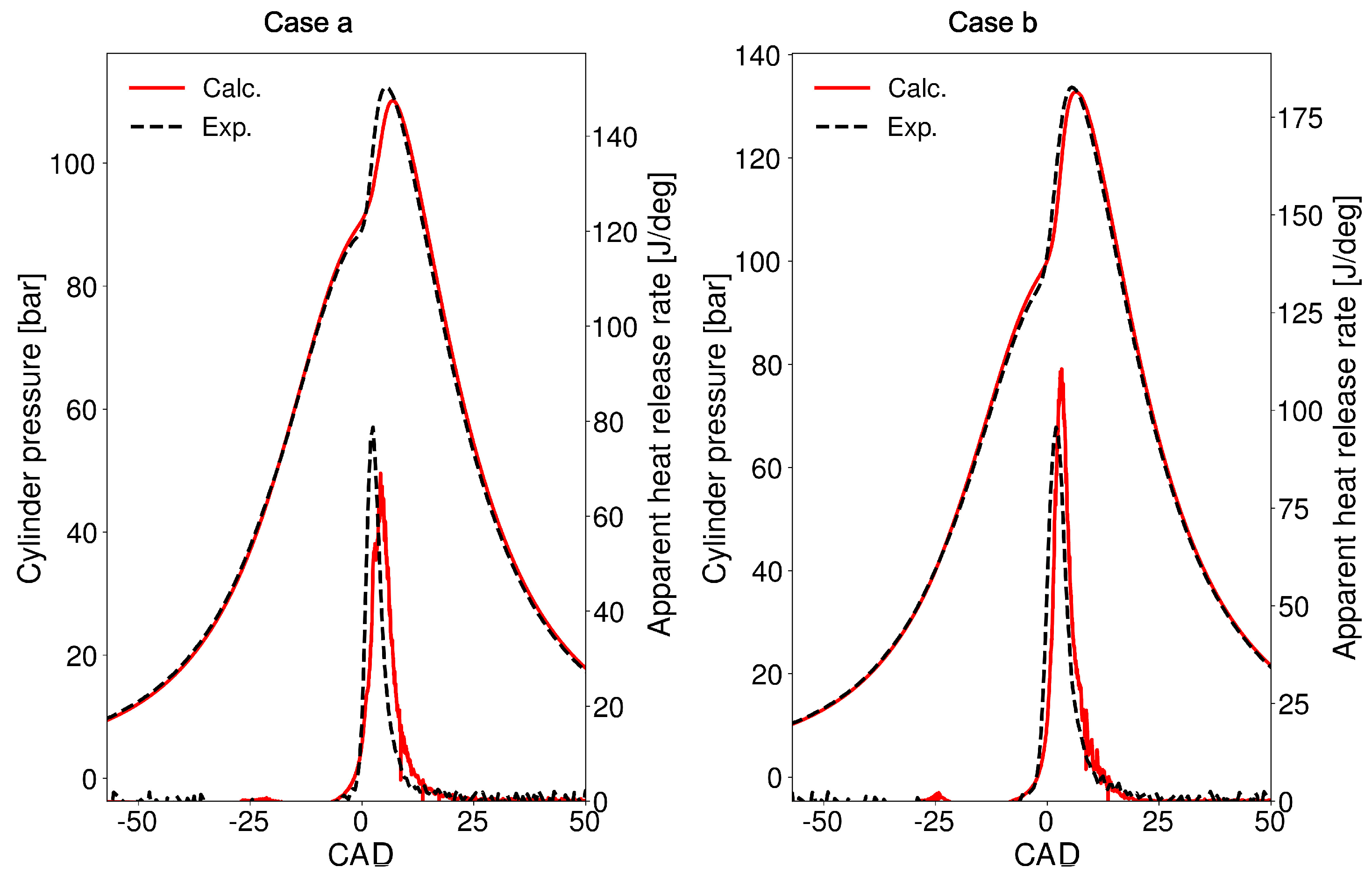
3.2.5. Validation of the CFD Model

Two relevant engine operating conditions were selected to validate the the numerical model against experimental data.

Table 3. Operating condition specifications as initial and boundary conditions for CFD calculations.

Case	a	b
$m_{f,tot}$ [mg]	13.5	19
PFI [%]	29.6	76.3
SOI [CAD]	−30	−32
$T_{f,DI}$ [K]	663	638
$P_{DI}$ [bar]	300	300
$\lambda$ [-]	5.1	4.15
$P_{IVC}$ [bar]	2.3	2.3
$T_{IVC}$ [K]	378	380
Speed [rpm]	2000	2000
GIE [%]	39.6	42.7

details the operating conditions of the three cases: the case named a represents the low load point; meanwhile, the case b is a medium load case. Regarding the fuel temperature $T_{f,DI}$, in the CFD simulations, it is related to the temperature at the exit of the injector nozzle. Meanwhile, in the experiments, it corresponds to the value measured with the thermocouple after the heating resistance, immediately before the injector.

The comparisons between the simulated and experimental in-cylinder pressure and heat release rate are shown in Figure 5. Computed traces are in good agreement with the experimental ones. It is of particular interest how the simulations are able to correctly predict the ignition delay and the peak of HRR; therefore, the model captures the evolution of the combustion reactions and the fuel distribution. The chemical mechanism is characterized by cool flames around −25 CAD, and this intensity is overestimated with respect to the experimental results.

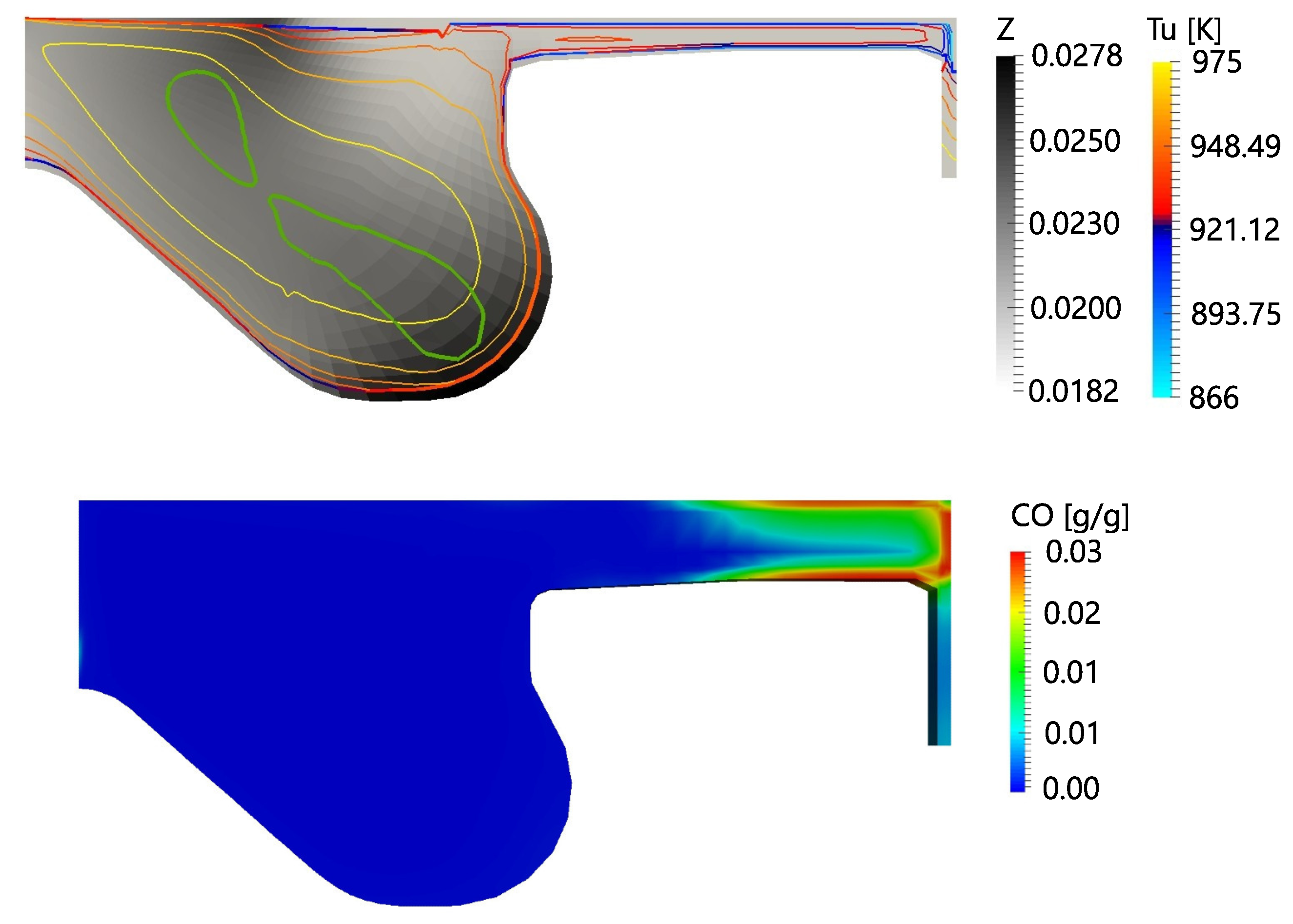
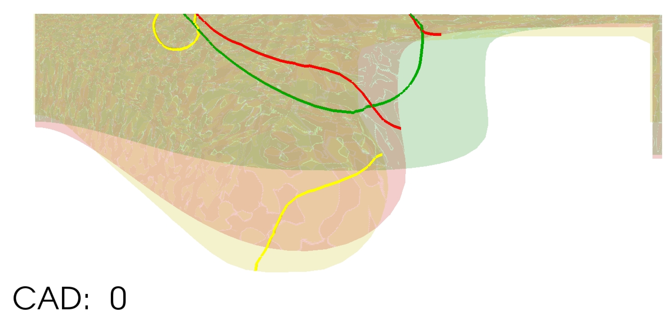
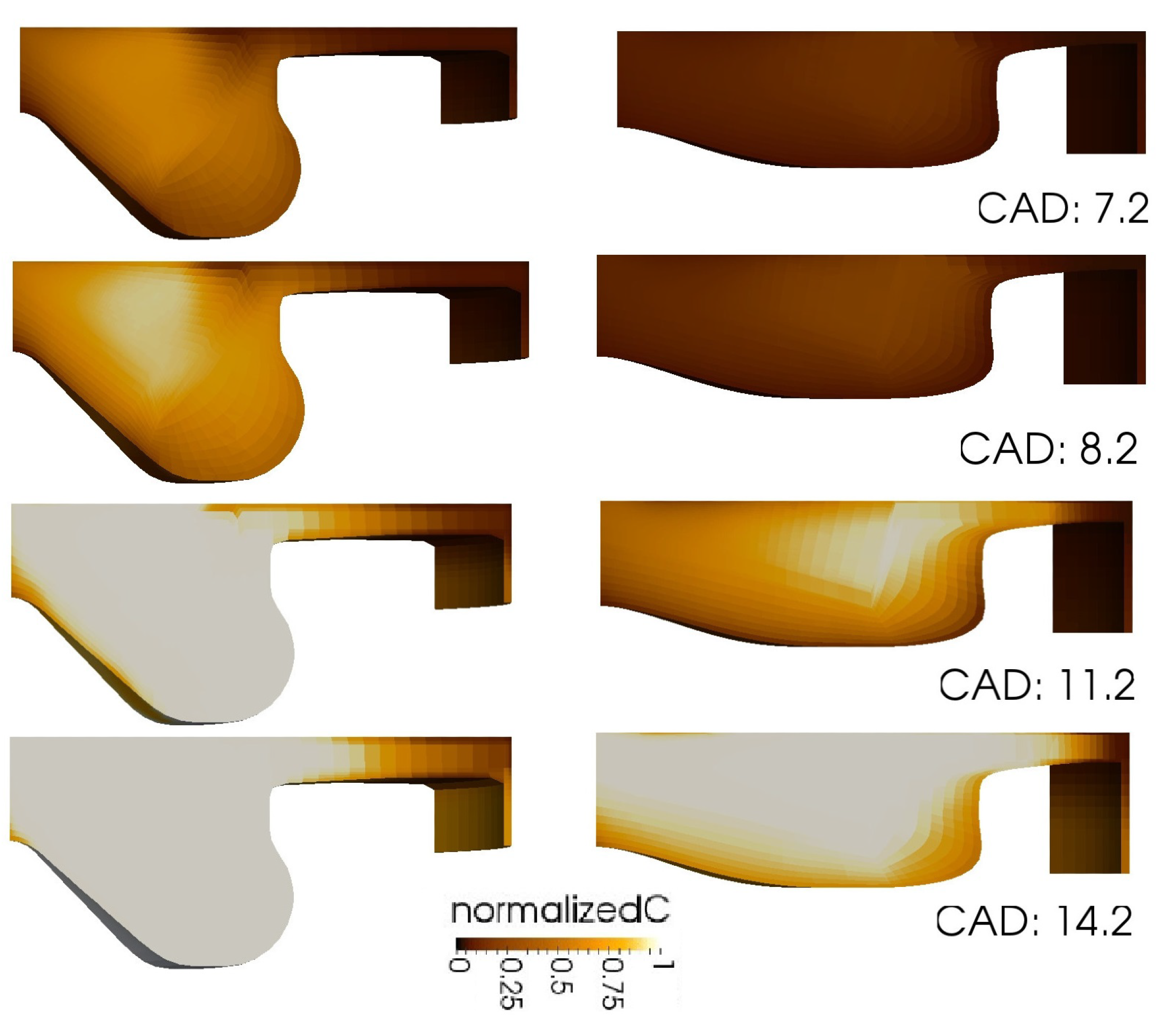
The main effect of the direct injection is to create a rich region in the piston bowl. Here, the richer mixture is the first to ignite, and the combustion diffuses towards the rest of the combustion chamber, as represented in Figure 6.

The direct injection does not reach the squish region. Here, the resultant homogeneity of the mixture could promote a knocking-like combustion in this region when the load increases, since this area tend to ignite simultaneously. On the other hand, close to TDC, the influence of the thermal boundary layer and the heat exchange with the walls are relevant. These properties entail a lower unburned gas temperature that hinders the combustion promoting $CO$ and $HC$ emissions close to the cylinder wall (Figure 6).

It is now clear that the diesel-like piston geometry is not optimized for this kind of premixed combustion, since the direct injection only reaches the volume inside the piston bowl.

An optimized piston geometry for RCCI technology has been proposed in [22,23]. The authors observed that hydrocarbon emissions are reduced by a piston design with a small squish distance and large bowl volume. Then, the next step of this study is to find a suitable combustion chamber architecture that maximizes the performance of the TCRCI concept.

3.2.6. Set-Up Difference between Validation and Optimization Cases

The set-up used for the optimization simulations differs from the validation case due to the necessity to speed up the computational time and to automatically mesh a large variety of piston geometries. It follows that a fully automatized mesh and coarser time steps are used.

In particular, the time step was doubled during the injection, and it is increased by five times between the end of injection and the start of combustion (

Table 4. Time discretization for the validation and PSO cases.

Start Time	−153	−36	−27.5	−5	30	50
$\mathrm{\Delta }CAD$ Val.	0.125	0.0005	0.01	0.01	0.125	0.125
$\mathrm{\Delta }CAD$ PSO	0.125	0.001	0.05	0.01	0.05	0.125

).

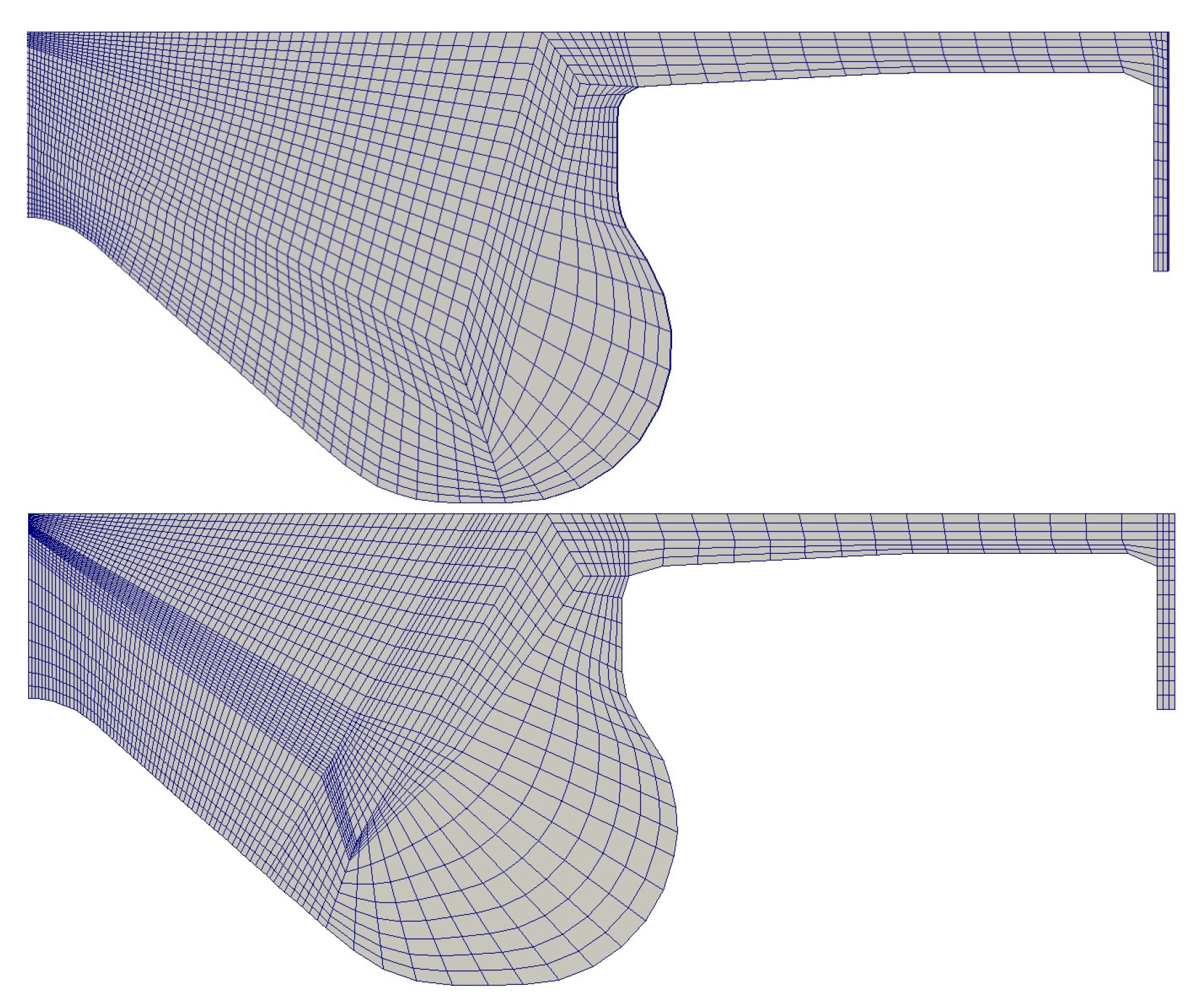
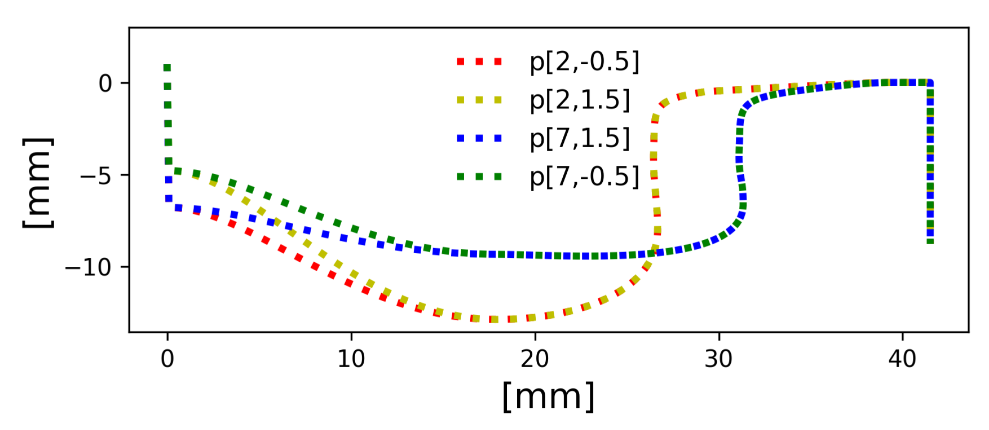
Figure 7 shows the changes in the mesh configuration. The image at the top of Figure 7 represents a 60 degree sector, and it is manually adjusted to achieve the best possible configuration. The grid size was selected after a preliminary mesh independence analysis based on the previous experience of the authors [5,6]. The domain has around 65,160 cells at TDC position [24,25]. The bottom image shows the automatic mesh generated to perform the optimization process in order to reduce the time required for each simulation.

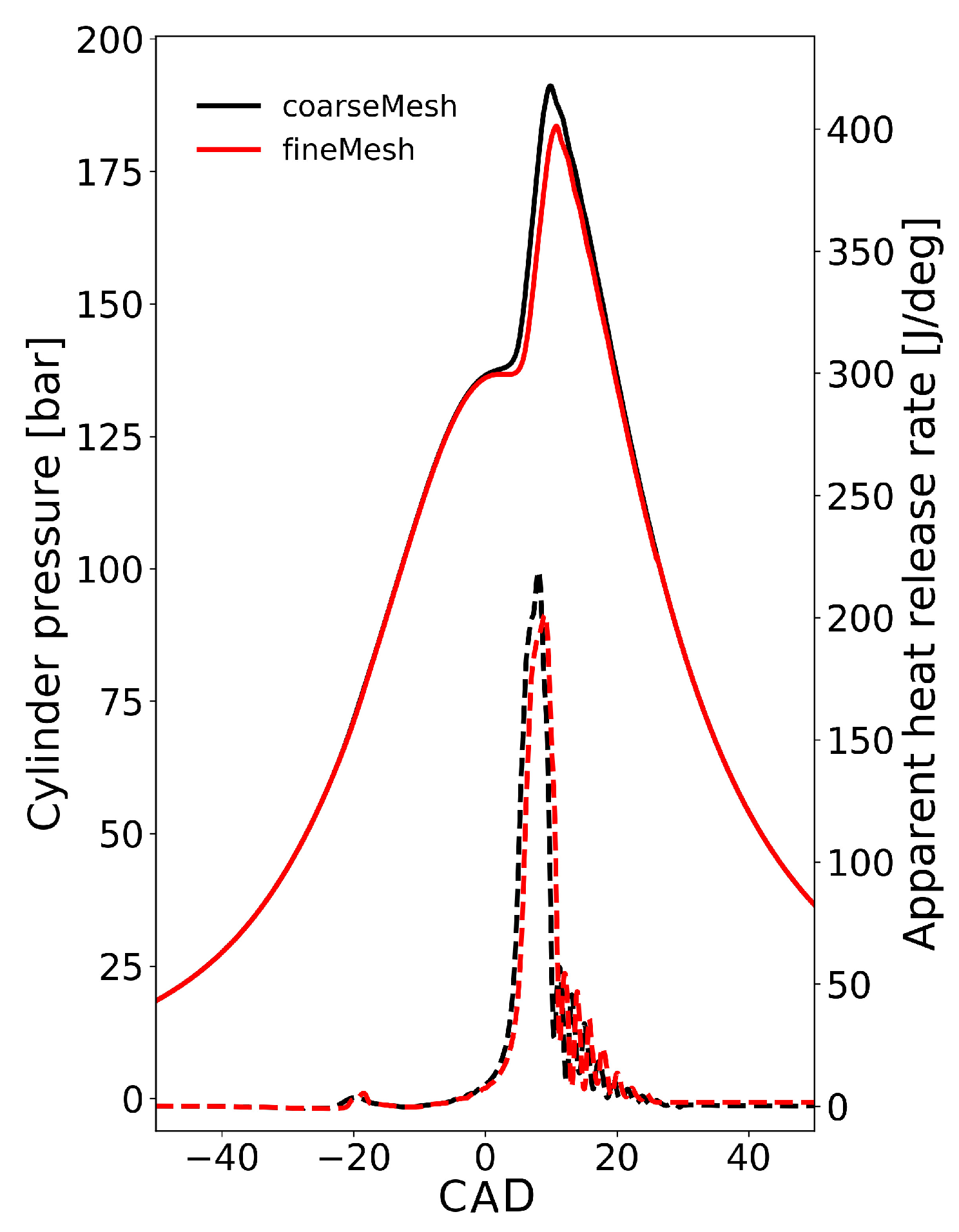
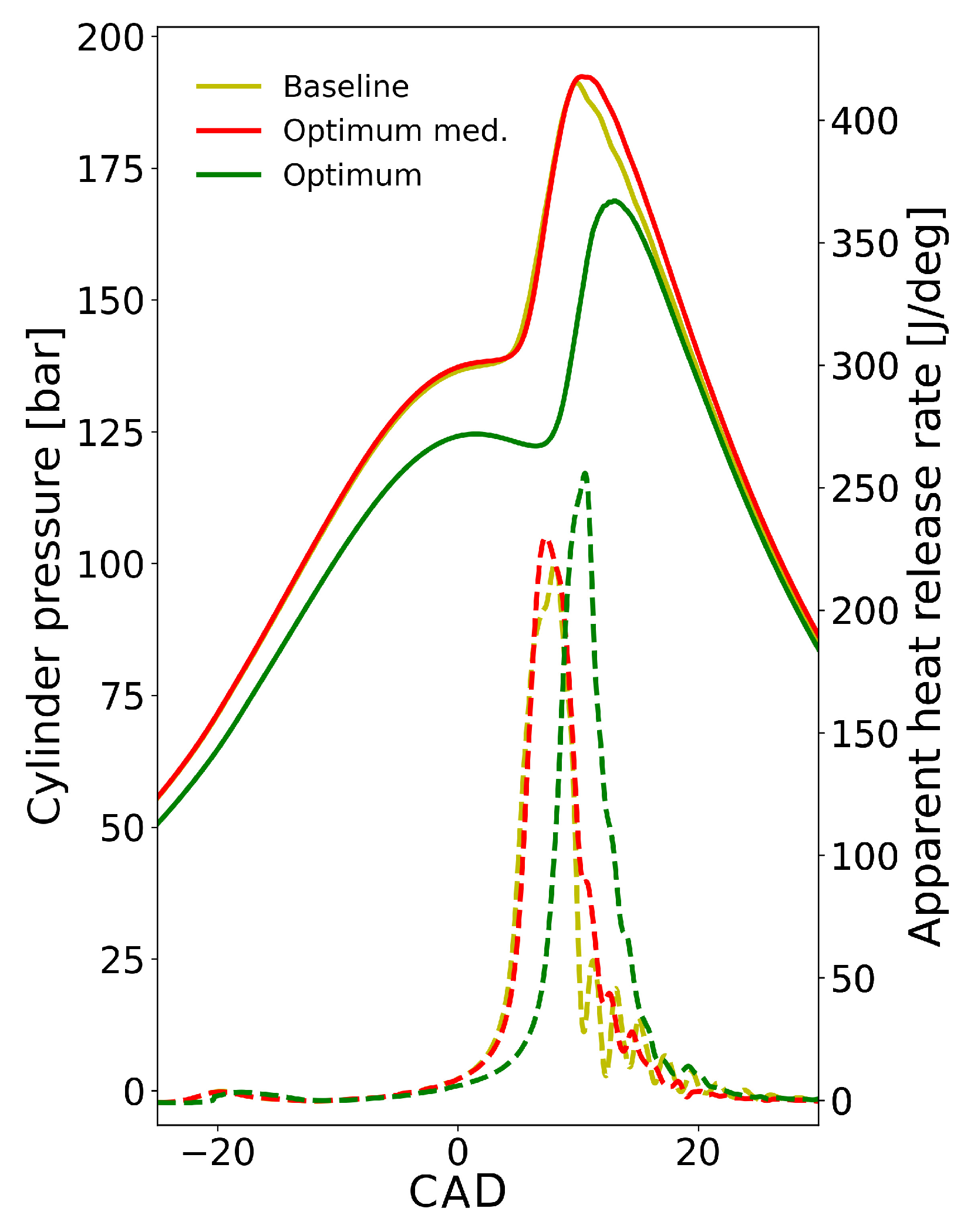
These changes do not significantly affect the simulation results, as represented by the comparison of the traces shown in Figure 8. The only small discrepancy is in the ID. This difference has been considered acceptable since the combustion is chemically driven, and therefore the combustion is sensitive to small local differences. On the other hand, the simulation configuration adopted for the PSO reduces almost half of the computational time required, which was reduced from 40 h to 24 h when decomposing the simulation in eight cores.

3.3. Particle Swarm Optimization

PSO is a population-based optimization technique that iteratively optimizes a candidate based on their previous information and that of its neighbors with regard to a given measure of quality. This algorithm is defined as meta-heuristic since it does not require assumptions of the problem and it is able to search very large spaces of candidate solutions. The mathematical formulation is presented here:

Given a function f

$$f:{\mathbb{R}}^D\to \mathbb{R}$$

(5)

The minimization problem consists of

$$x_{opt}|f\left(x_{opt}\right)\le f\left(x\right)$$

(6)

The D-dimensional domain of f is the search space. The search space is mapped by a fixed number of position vectors called particles. The set of particles takes the name of swarm X:

$$X=[x_1,\dots ,x_N]$$

(7)

For each t-iteration, the i-particle position is updated based on the velocity vector $v_i(t+1)$:

$$x_i(t+1)=x_i\left(t\right)+v_i(t+1)$$

(8)

where the velocity vector is computed based on the relative position of the particle with respect to the current best position of $x_i$: $p_i$, and the global best positions among all the swarm particles g:

$$v_i(t+1)=w{\beta }_i\left(t\right)+c_1\tau (p_i-x_i\left(t\right))+c_2\gamma (g-x_i\left(t\right))$$

(9)

where w is the inertia weight, $c_1$ is the individual weight, and $c_2$ is the social weight. $\beta ,\tau$ and $\gamma$ are random vectors uniformly distributed between 0 and 1. The used algorithm differs from this basic formulation since it divides the swarm into two subgroups that differ for the definition of the velocity: conquerors and explorers particles. The conquerors follow the formulation described above and tend to consistently converge to a minimum. The explorers look into the unexplored or less attractive region of the search space thanks to the application of the Novelty Search concept. For a deeper explanation of the implementation of the algorithm and its performance analysis, please refer to the work of Rodrıguez et al. [26]; from which the small explanation reported above is taken. The same algorithm has been successfully applied to the optimization of a CI engine operating with OME fuel [24].

3.4. PSO CFD Integration

The PSO is coupled to 3D CFD simulations, and it is therefore necessary to integrate the particle elements to the CFD software and to convert the outputs to a synthetic 1D value via the definition of a merit or objective function. The particle vector elements are the boundary conditions of interest for the CFD simulations and the parameters used to generate the bowl profile. In order to modify the boundary condition for each generation, different Python routines have been written, which are able to take as input the new parameters defined by the optimization algorithm and update the simulation control files.

Piston Bowl Geometry Generator

The piston bowl geometry is generated using the Bézier polynomial curves. For this purpose, a number of independent parameters are defined which are the control points that describe the evolution of the bowl curve. These parameters are dimensionless and have their own ranges and limits. Depending on the complexity of the desired geometry, the number of parameters can range from two to six. This parameterization allows a large flexibility of the bowl geometry. The squish height is adjusted to keep the volume and thus the Compression Ratio (CR) constant; this parameter is limited between 0.6 and 1.5 mm, suggested as typical values for a diesel piston design [27]. The optimum geometry is expected to be far from the original diesel configuration. Furthermore, since the Start of Injection (SOI) is anticipated and there is a relevant time for the mixing processes, it is not necessary to have a complex piston bowl geometry. These are the reasons behind the choice to use only two parameters, which grant a good geometrical flexibility and keep a small number of total parameters, reducing the total optimization time. The boundaries of the search space of the possible bowls are represented in Figure 9.

3.5. Definition of the Parameters to Optimize

The parameters to optimize are presented in this section. There are nine parameters in total, and they have been selected due to the high influence on the engine performance:

• Hardware: two geometrical parameters to define the bowl profile, and one that specifies the spray included angle.
• Air management: pressure and temperature at IVC and Exhaust Gas Recirculation (EGR) level.
• Fuel management: the distribution between direct and port injected fuel, and the direct injected fuel temperature.

Some observations regarding the parameters are proposed below:

• The pressure and temperature are changed independently; therefore, the total in-cylinder mass and the equivalence ratio vary. Then, it is necessary to update the mixture fraction at IVC for each case to maintain the premixed fuel mass constant. This procedure is made according to the ideal gas equation.

  $$\frac{P·Z}{T}=constant$$

  (10)
• The distribution of direct and port-injected fuel affects different fields. It influences the mixture fraction at IVC:

  $$\frac{Z}{PF{I}_{\%}}=constant$$

  (11)
  It also affects the injected mass; since the injector is gaseous and is chocked in the ideal gas hypothesis, the steady mass flow rate is kept constant, and the injection duration is adapted to the total mass. As a consequence, the time-step division is adapted to the new injection duration.
• The EGR variation is controlled by changing the chemical table. The reason is that the EGR level affects the environment composition, which is initialized in the table inputs. The EGR level discretization step is 2% to reduce the number of total tables.

The search space for each parameter is summarized in

Table 5. Boundaries for each parameter.

	Lower	Upper
geom. $p_1$	0.268	7.069
geom. $p_2$	−0.869	1.5
SA [°]	160	170
SOI [CAD]	−45	−30
$T_{DI}$ [K]	570	700
$PFI$ [%]	70	86.5
$T_{IVC}$ [K]	378	388
$P_{IVC}$ [bar]	3	3.6
$EGR$ [%]	20	36

:

The flexibility of the geometric parameters and the spray angle are limited by the meshing process because it is difficult to achieve an acceptable mesh quality for wide piston bowls and narrow spray inclusive angles. The thermodynamic conditions at IVC are centered on the baseline values, and the range of temperature might seem small, but the sensitivity of this type of LTC technology is large, as the combustion is chemically driven. The upper limit of $PF{I}_{\%}$ is close to the baseline since the injected fuel mass is already very small and the injector is already working almost in the ballistic region. It is thus technically difficult to further decrease the direct injected mass. The upper limit of SOI has been chosen to produce an effective fuel stratification. The bottom limit of the fuel temperature has been chosen to be 20 K above the critical point to be sure to have a super-critical injection.

3.6. Output and Merit Function

This optimization is based on maximizing the efficiency and restricting the maximum pressure and pressure rate. The merit function is configured to favor an efficiency increase; meanwhile, it limits the maximum pressure rate. The merit function is formulated considering a different weight for each parameter. In this case, the efficiency is most important, while the pressure indicators are used only as restrictions.

3.6.1. Efficiency

Since the boosting pressure is different for each tested particle, it is necessary to consider the pumping losses. A loss parameter is introduced to account for the energy required to heat the fuel, since both the direct injected fuel mass and temperature change.

$$NIE=GIE-los{s}_{pump}-los{s}_{fuel}$$

(12)

The Gross Indicated Efficiency (GIE) is computed directly from the pressure integration in the volume using the rectangle rule:

$$GIE=\frac{{\int }_{IVC}^{EVO}pdV}{m_f·LHV}$$

(13)

The pumping losses are computed using a model based on the turbocharging equation [1] as follows:

$$los{s}_{pump}=\frac{(p_{exh}-p_{int})V}{m_f·LHV}$$

(14)

This coefficient ranges almost linearly with the pressure at IVC within three and five percentage points. The constants of the model have been tuned based on the experimental pressure traces of an operating condition very close to the baseline.

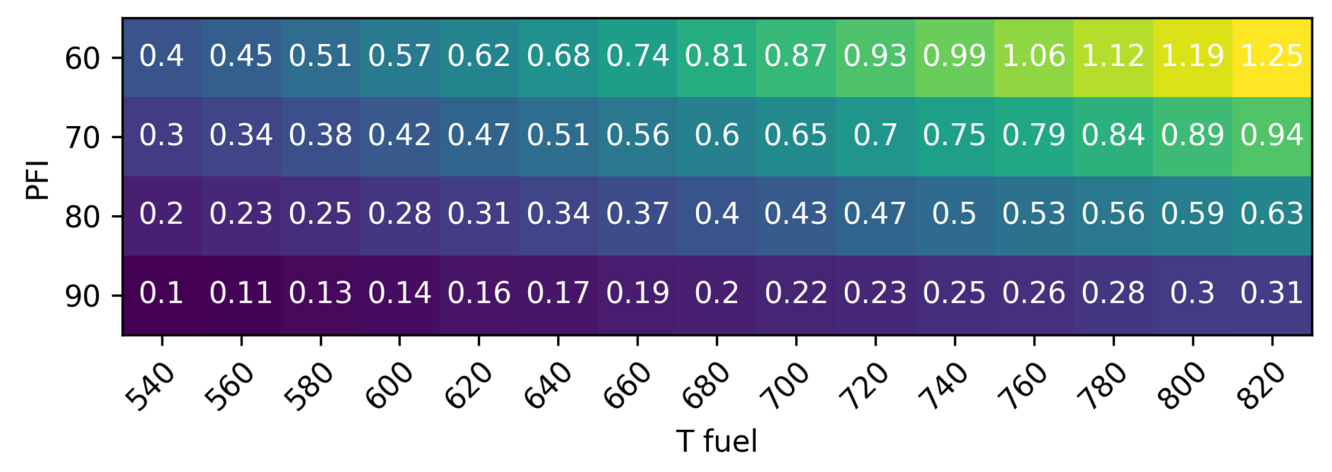
Moreover, the amount of energy required to heat the fuel is also considered in a coefficient. This parameter is a function of the fraction of direct injected fuel, the thermo-physical properties and the final fuel temperature. Note that this formulation does not take into account the losses in the heating process. The equation for the efficiency losses due to the fuel heating is the following:

$$los{s}_{fuel}=\frac{m_{DI,f}·Q\left(T_f\right)}{m_f·LHV}=(1-PF{I}_{\%})\frac{Q\left(T_f\right)}{LHV}$$

(15)

Figure 10 presents a map of this parameter for iso-octane in the range of interest for this application. The heat is computed with CoolProp [28] considering a constant pressure equal to the injection pressure (300 bar) and a base fuel temperature equal to 380 K. It is possible to notice that the maximum loss in the considered range is 1.24%. It is worth noticing that the energy required could be reduced by exploiting the residual thermal energy of the exhaust gasses.

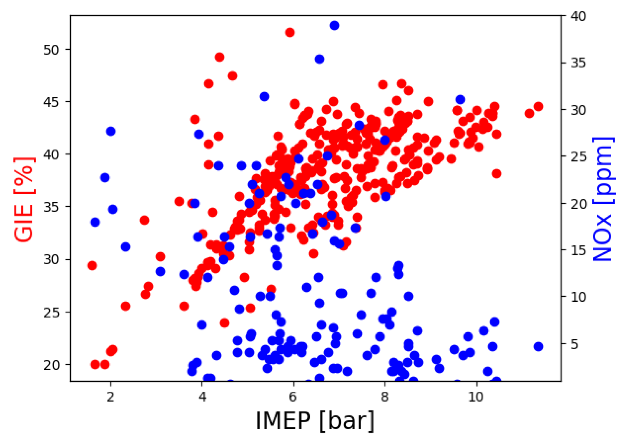
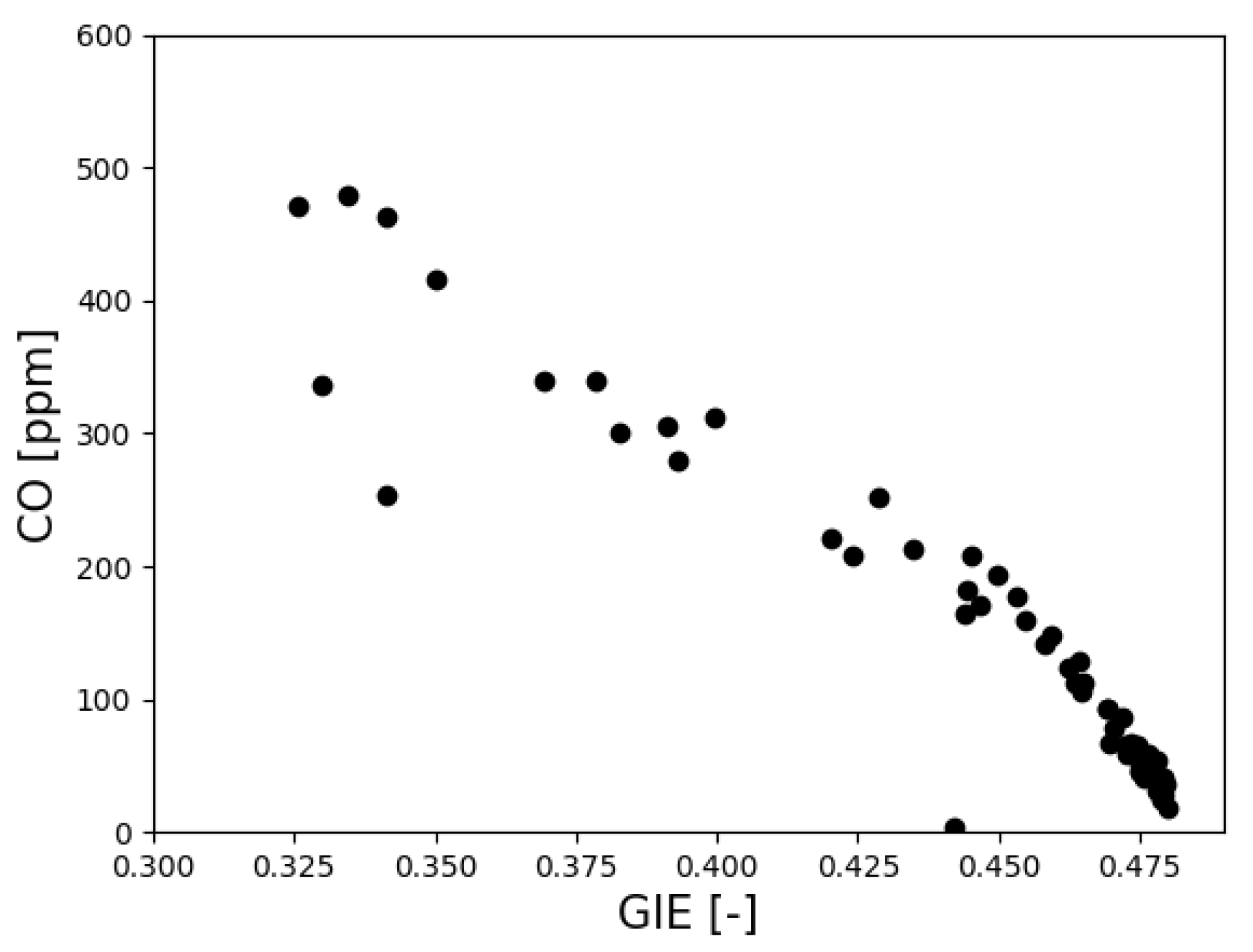
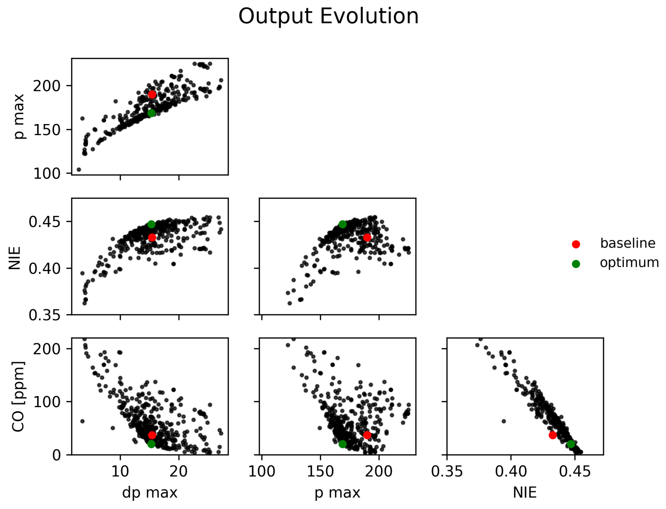
It must be noticed that pumping losses are one order of magnitude bigger than the fuel heating losses. $CO$ emissions are not considered in the merit function since its evolution is strictly correlated to the efficiency, as is possible to notice in Figure 11.

3.6.2. Maximum Pressure Rate

Knock is the effect of an improper combustion phenomenon. It produces pressure waves that travel inside the cylinder and are reflected by the walls, which result in an oscillatory behavior of the pressure trace. The combustion model used in this work is not able to directly model the detonation, and an index proportional to the knock propensity must be therefore introduced. One of the most often used is the Ringing Index proposed by Eng et al. [29], which is the result of a theoretical analysis on the pressure waves.

$$RI=\sqrt{\frac{R·T_{max}}{4·P_{max}^2}}·{\left(\beta ·\frac{dP}{d{t}_{max}}\right)}^2$$

(16)

where $\beta$ is a scale factor determined from the experimental data. In [30], $\frac{dP}{d{t}_{max}}$ is directly used as limiting parameter, since the scaling factors $T_{max}$, $P_{max}$ are used to include engines with different characteristics. These parameters have a small influence for similar operating points, since they have the same trend. It follows that the pressure rate is directly used as an index. Furthermore, it has been chosen to move from the time to the angular coordinate, since the engine speed is constant.

3.6.3. Merit Function

The performance of the new combustion system obtained from each case of the optimization process is evaluated by means of the merit function that considers the efficiency, maximum pressure and maximum pressure rate simultaneously. The merit function equation is described as follows:

$$MF=0.75·f\left(\eta \right)+0.02·f\left(p_{max}\right)+0.02·f\left(d{p}_{max}\right)$$

(17)

where

$$f\left(\eta \right)=\left\{\begin{array}{cc}\frac{\eta }{{\eta }_{lim}},\hfill & \mathrm{if}\eta >{\eta }_{lim}\hfill \\ \frac{\eta }{{\eta }_{lim}}+1000·{({log}_{10}\left(\eta \right)-{log}_{10}\left({\eta }_{lim}\right))}^2,\hfill & \mathrm{if}\eta <{\eta }_{lim}\hfill \end{array}\right.$$

$$f\left(p_{max}\right)=\left\{\begin{array}{c}\frac{p_{max}}{p_{ma{x}_{lim}}},\mathrm{if}{p}_{max}<p_{ma{x}_{lim}}\hfill \\ \frac{p_{max}}{p_{ma{x}_{lim}}}+100·{(p_{max}-p_{ma{x}_{lim}})}^2,\hfill & \mathrm{if}{p}_{max}>p_{ma{x}_{lim}}\hfill \end{array}\right.$$

$$f\left(d{p}_{max}\right)=\left\{\begin{array}{cc}\frac{d{p}_{max}}{d{p}_{ma{x}_{lim}}},\hfill & \mathrm{if}d{p}_{max}<d{p}_{ma{x}_{lim}}\hfill \\ \frac{d{p}_{max}}{d{p}_{ma{x}_{lim}}}+10·{(d{p}_{max}-d{p}_{ma{x}_{lim}})}^2,\hfill & \mathrm{if}d{p}_{max}>d{p}_{ma{x}_{lim}}\hfill \end{array}\right.$$

It can be noticed that the efficiency function has a different formulation with respect to the other function: the logarithm is used to increase the relevance of this parameter. For the same reason, the efficiency has a coefficient much greater than the other ones. The limit efficiency is the baseline one; it has been chosen to give an upper tolerance of $10\%$ with respect to the baseline condition to the limit of pressure and pressure rate. The reason is that the baseline condition is far from the limits of the engine (24 bar/CAD and 240 bar). As a consequence, even if it is better to control the maximum pressure rate, a value slightly larger than the baseline is acceptable.

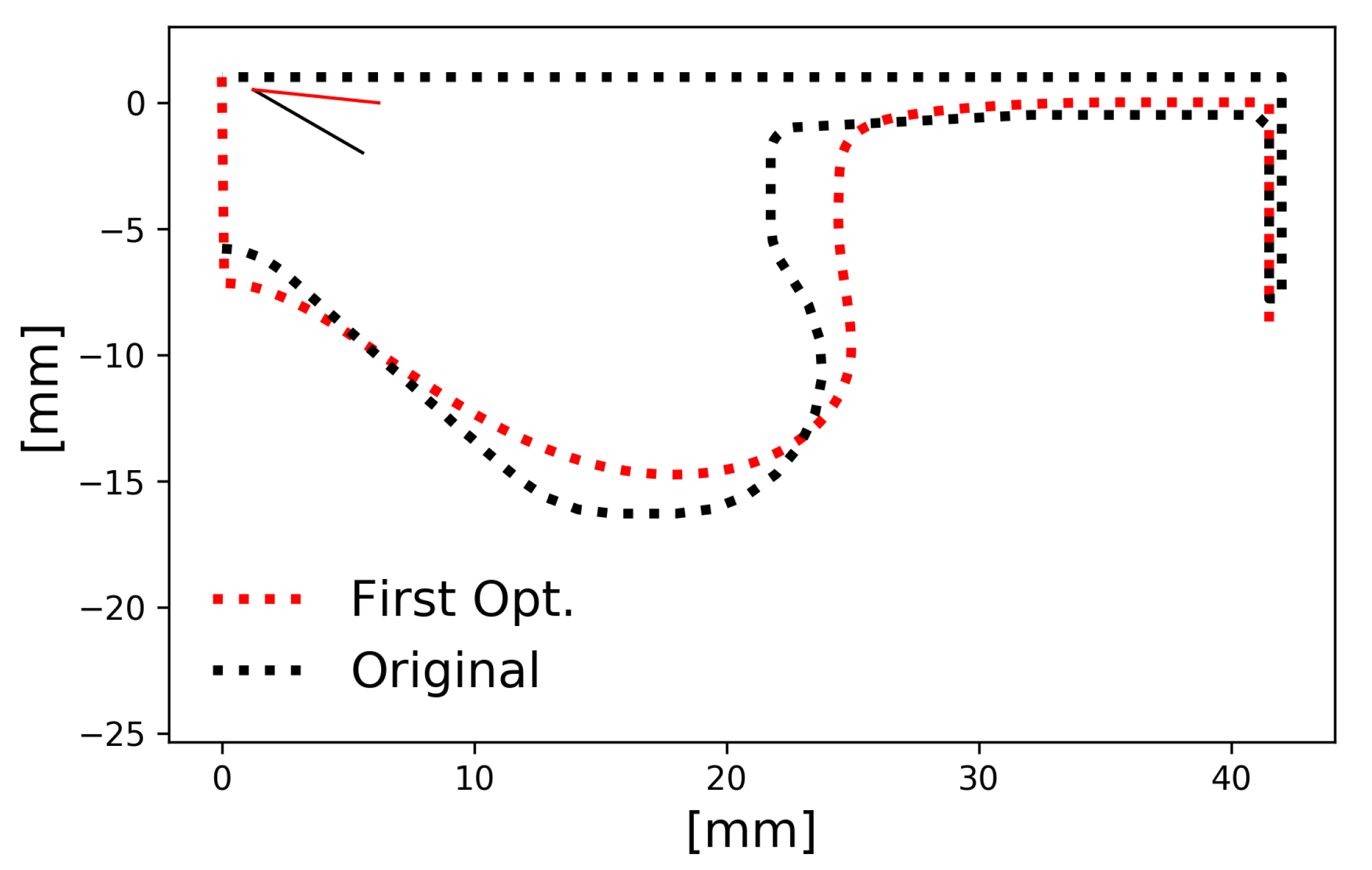
3.7. Baseline Condition

This optimization is made in a relatively high load and high speed condition, since the high load conditions are the most critical for LTC engines, with the charge being premixed and prone to knock at a high in-cylinder temperature and with richer mixtures. The peculiarity of this optimization is that the baseline condition is not directly the case with the diesel hardware but is the result of the previous intermediate optimization. This choice has been imposed by the original spray angle (120°), which limits the mesh quality when the bowl diameter increases. The purpose of the intermediate optimization is to find an intermediate hardware that allows a larger flexibility. This optimization involves only the piston geometry, the spray angle and a small $T_{IVC}$ flexibility to adjust the combustion phasing with the variation of the mixture distribution.

Intermediate Optimization

The baseline operating condition in the diesel hardware is characterized by the parameters specified in

Table 6. Operating condition and performance parameter of the baseline case and intermediate optimization.

		Baseline	Intermediate Optimization
Input	SA [°]	120	168.9
	SOI [CAD]	−40	−40
	$T_{DI}$ [K]	640	640
	$PFI$ [%]	86.5	86.5
	$T_{IVC}$ [K]	384	384
	$P_{IVC}$ [bar]	3.3	3.3
	$EGR$ [%]	30	30
	Speed [rpm]	3000	3000
Output	$p_{max}$ [bar]	185	190
	$d{p}_{max}$ [bar/CAD]	13.7	15.4
	GIE [%]	45.16	47.6
	$CO$ [%]	0.416	0.369

.

This preliminary optimization involves five bowl geometry parameters, the spray angle, which ranges from 120 to 170 CAD, and the temperature at IVC. The pressure is linked to the temperature by the ideal gas equation to keep the total mass constant. The Merit Function (MF) definition is the same as the main case; however, it directly uses the GIE, since the direct injected (DI) fuel mass is constant and the pressure variation at IVC is limited. The best achieved configuration is characterized by the same initial temperature, a slightly wider piston bowl (at the limit fixed for this optimization) and a much wider spray angle. The combustion chamber geometry is shown in Figure 12, while the new operating conditions are summarized in Table 6.

The new spray angle allows us to enrich the squish region as well, improving the combustion efficiency and thus the overall efficiency. Since this is an intermediate configuration, the analysis is limited to the small consideration made in this section. Moreover, the new SA allows a much larger flexibility in the meshing process in case of wider piston bowl geometries.

4. Results and Discussion

The optimization results are presented and discussed here. First, a convergence analysis is performed; afterwards, the best position and the influence of the hardware and operating parameters are deeply analyzed.

4.1. Optimization Results

The first step of the analysis is the assessment of the algorithm’s convergence. It is possible to see in Figure 13 that the best position found by the algorithm continuously decreases with the number of iterations. The convergence is reached rapidly in the first part of the optimization. From iteration 200 to 360, the best point almost does not improve. At iteration number 360, there is the last big decrease of the MF, which later tends to remain constant until the optimization is stopped, based on the analysis of the evolution of each parameter.

Figure 14 shows the evolution of the single outputs, considering only the best particle for each generation. The horizontal red line represents the baseline condition.The improvement of the NET Indicated Efficiency (NIE) is clear starting from the base level. This is both a consequence of the increase of GIE and the lower pumping losses. Furthermore, the maximum pressure rate is always below the baseline case. A significant improvement is achieved regarding the emission of $CO$—a clear signal of the increase of the combustion efficiency.

It is possible to see the evolution of the PSO coupling the different outputs. For every pair of outputs, the optimum is always on the boundary of the explored domain in Figure 15. Furthermore, it is clear that the efficiency evolution as a function of $p_{max}$ and $d{p}_{max}$ is in a Pareto front. The best point is the best trade-off available according to the definition of the MF coefficients, since it is the point with the minimum pressure value that grants an efficiency value very close to the maximum one. The choice of which point is the optimum on the Pareto front is based on the definition of the merit function, and changing its definition would bring a different optimum. Looking at the efficiency–$CO$ scatter plot, the quality of the found solution is clear, since the best position is very close to the minimum of the emission–efficiency front and quite far from the baseline.

4.1.1. Piston Geometry Evolution

The evolution of the piston shape of the best particles for each generation is presented in Figure 16. The bowl monotonously moves towards a wider piston bowl until it reaches the best point, close to the limit available for this generation ($p_{1,opt}=5.81$); furthermore, the combination of the two geometrical parameters tends towards a straight bottom of the bowl.

The fuel stratification at TDC of the baseline, intermediate and final optimum is shown in Figure 17.

The rich regions of the baseline and the intermediate optimum are close to the piston wall, since the small squish diameter does not allow the injection to diffuse freely inside the combustion chamber.

To understand the reasons for this evolution, particles with all parameters equal to the optimum case (with a 2% error) except for the two piston bowl cases were extracted from all the simulated particles. The 48 cases resulting from this procedure differ only in the piston bowl geometry. This analysis (Figure 18) shows the relevance of the piston bowl geometry. Wider piston bowls provide a higher efficiency without an increase of the peak of pressure rate. The geometry affects the fuel distribution, the temperature stratification and the heat exchange. The heat exchange decreases due to the smaller area of the wall surfaces. It is significant in this regard that the best point is also the one with the smallest bowl perimeter.

4.1.2. Optimum Case

This section analyzes the best case found with the optimization process.

Table 7. Operating condition and performance parameter of the optimum case.

		Baseline	Optimum
Input	SA [°]	168.9	165.4
	SOI [CAD]	−40	−32.8
	$T_{DI}$ [K]	640	669
	$PFI$ [%]	86.5	86.5
	$T_{IVC}$ [K]	384	382
	$P_{IVC}$ [bar]	3.3	3.0
	$EGR$ [%]	30	22
	Speed [rpm]	3000	3000
Output	$p_{max}$ [bar]	190	168.8
	$d{p}_{max}$ [bar/CAD]	15.4	15.4
	NIE $[\%]$	43.3	44.7
	GIE $[\%]$	47.6	48.0
	CO [mg]	0.407	0.136

presents the comparison between the engine configuration of the optimum and the baseline. The optimum configuration is quite far from the baseline. This implies that the original combustion system was working far from its true potentiality. The final configuration is characterized by an increase of the net efficiency of 1.3% with respect to the intermediate optimum, achieved by an increase of the GIE (0.4%) and the decrease of the pumping loss, since the initial pressure has been decreased by 10% (from 3.3 to 3.0 bar). The combustion efficiency is significantly improved, as testified by the significant reduction of the $CO$ emissions.

The colder mixture and the different fuel distribution delay the combustion by almost 5 CAD with respect to the baseline case even if the peak of pressure rate is almost constant (Figure 19), as a result of the combined effect of the other parameters.

Another benefit of the smaller squish volume is the absence of a homogeneous combustion in the squish volume, which causes the oscillatory evolution of the HRR at the end of combustion in the baseline case. This deficient evolution is already reduced in the intermediate optimum and is almost absent in the final one. The comparison of the combustion evolution between the baseline and the optimum cases are shown in Figure 20.

4.1.3. Parametric Analysis

This section presents the results of a parametric study to analyze the effect of every single parameter on the overall final result. For this purpose, starting from the baseline condition, one parameter at a time has been changed with its optimal value until the optimal condition is reached. The Port Fuel Injection (PFI) percentage and the spray angle have been neglected from this analysis since they are very close to the original one. The limit of this kind of analysis is that it is order dependent, since the combustion problem is highly non linear. It has been chosen to firstly consider the hardware parameter (bowl geometry, SA) and later the operating parameters (EGR, $P_{IVC}$, SOI, $T_{IVC}$ and $T_f$). Figure 21 presents the energy diagram evolution. For clarity, the losses of second order—unburned fuel and the energy used to heat the direct injected fuel—have been grouped into the other losses entry. Moreover, Figure 22 shows the evolution of the merit function.

Based on the results presented in Figure 21 and Figure 22 some remarks can be made.

• The introduction of the new piston geometry has a major benefit on the use of the fuel energy. The benefits are present in all the loss sources, but the more relevant are linked to the heat exchange (minor piston perimeter) and a reduction of the heat loss in the exhaust gasses. Notice that the effect of the reduction of the piston surface area is high enough to compensate the increase of the peak of temperature and pressure. However, this new configuration is characterized by a higher peak of pressure rate.
• The change of the fuel distribution followed by the introduction of a more open SA allows the peak of the pressure rate to be decreased without significantly penalizing both the gross and the net indicated efficiency. However, the reduction of the pressure rate is not sufficient. Therefore, it is necessary to vary the other operating parameters.
• The introduction of a lower EGR level significantly advances the combustion and increases the peak of HRR, since the decrease of the inert gas fraction in the mixture decreases the ID. The earlier combustion decreases the combustion losses and increases the heat transfer; the net indicated efficiency therefore has a limited growth. This condition is however characterized by the higher objective function since both the peak of pressure and pressure rate significantly exceed the baseline value. It is thus necessary to delay the combustion phasing.
• The reduction of $P_{IVC}$ decreases the in-cylinder mass of 9%; the equivalence ratio therefore increases since the fuel mass is kept constant. The higher equivalence ratio also promotes a larger peak of HRR, and the ignition delay increases. The consequence is that this configuration solves the peak of pressure problem but is not able to significantly decrease the peak of pressure rate. Lastly, the pumping loss is decreased by 1%, which is the main factor responsible for the improvement of the net indicated efficiency.
• The new fuel distribution deriving from the different SOI delays the start of the combustion. This is however not sufficient to bring the peak of pressure rate below the baseline case.
• A lower $T_{IVC}$ allows the pressure rate to be decreased below the baseline, at the price of a combustion efficiency detriment and heat loss in the exhaust gasses consequent to the delayed combustion.
• Finally, the change of the fuel temperature has a small influence on the combustion evolution, since the injected mass is small, and the difference in this value is only 30 K.

In order to conclude the analysis, a direct comparison between the baseline operating condition operated in the diesel hardware and the optimum result is performed. The improvement of the net indicated efficiency is 3%, and it is well distributed in a decrease of the combustion, heat transfer and pumping loss. The improvement of the combustion efficiency (0.66%) is, as already discussed, linked to the reduction of the squish volume. Looking at the evolution of the combustion of the baseline and the optimum case (Figure 23), it is possible to notice that even if the combustion in the optimum case starts 3 CAD after the baseline, it penetrates much faster in the squish volume. Since the normalized progress variable is lower than in the squish volume, this is the area with the main concentration of the unburned combustion products, such as $CO$ and $uHC$. It is now intuitive to understand why the emissions of $CO$ are reduced by the new geometry.

The decrease of the heat exchange (1.45%) is a consequence of the already discussed reduction of heat transfer. The lower initial pressure is responsible for the decrease of the pumping losses (1.2%).

5. Summary and Conclusions

In this study, a numerical methodology for optimizing an engine using the TCRCI combustion mode was presented. This work aimed to find a proper combustion system to improve the NIE and reduce the pollutant emissions of CO. The methodology applied was based on coupling CFD simulations and the PSO algorithm. The optimization was performed in two steps. The first considered the bowl geometry and IVC temperature, and the second included the air-management and injection system parameters. The main conclusions obtained from this investigation can be summarized as follows.

The optimized combustion system provided by this procedure is far from the baseline configuration, and it is characterized by an increase of the NIE, which moved from 41.14% to 44.7%, maintaining the same maximum pressure rate. This improvement has been achieved thanks to a flatter piston with a larger bowl diameter linked with a wider SA, a delayed SOI, lower EGR, $P_{IVC}$ and $T_{IVC}$. The causes of this net improvement are as follows:

• A smaller squish volume and thus higher combustion efficiency since the squish volume is the region where almost the totality of uncompleted combustion products are located.
• Smaller piston wall surface, with the same CR, and thus heat transfer losses.
• Decrease of pumping losses, thanks to smaller intake pressure.

Finally, $CO$ emissions were reduced due to the better combustion efficiency achieved.

References

1. Ferrari, G. Motori a Combustione Interna; Società Editrice Esculapio: Milan, Italy, 2016. [Google Scholar]
2. Krishnamoorthi, M.; Malayalamurthi, R.; He, Z.; Kandasamy, S. A review on low temperature combustion engines: Performance, combustion and emission characteristics. Renew. Sustain. Energy Rev. 2019, 116, 109404. [Google Scholar] [CrossRef]
3. Reitz, R.D.; Duraisamy, G. Review of high efficiency and clean reactivity controlled compression ignition (RCCI) combustion in internal combustion engines. Prog. Energy Combust. Sci. 2015, 46, 12–71. [Google Scholar] [CrossRef] [Green Version]
4. Lakshminarayanan, P.A.; Aghav, Y.V. Modelling Diesel Combustion; Springer: Berlin/Heidelberg, Germany, 2010. [Google Scholar] [CrossRef]
5. Gazzola, F. Evaluation of the potentials of Temperature Controlled Reactivity Compression Ignition combustion for efficiency increase in CI engines. J. Clean. Prod. 2022, 330, 129781. [Google Scholar]
6. C, V.; Murugesan, A.; Subramaniam, D.; Panneerselvam, N. An Experimental Investigation of Diesel Engine Fuelled with MgO Nano Additive Biodiesel—Diesel Blends. Bull. Sci. Res. 2019, 1, 28–34. [Google Scholar] [CrossRef] [Green Version]
7. Lehtiniemi, H.; Zhang, Y.; Rawat, R.; Mauss, F. Efficient 3-D CFD Combustion Modeling with Transient Flamelet Models. SAE Tech. Paper. 2008, 23. [Google Scholar] [CrossRef]
8. Dario Lopez Pintor, J.D.; Gentz, G. Φ-Sensitivity for LTGC Engines: Understanding the Fundamentals and Tailoring Fuel Blends to Maximize This Property. SAE Int. 2019. [Google Scholar] [CrossRef]
9. Lucchini, T.; Cornolti, L.; Montenegro, G.; D’Errico, G.; Fiocco, M.; Teraji, A.; Shiraishi, T. A comprehensive model to predict the initial stage of combustion in SI engines. SAE Tech. Pap. 2013, 2, 16. [Google Scholar] [CrossRef]
10. Lucchini, T.; Della Torre, A.; D’Errico, G.; Montenegro, G.; Fiocco, M.; Maghbouli, A. Automatic Mesh Generation for CFD Simulations of Direct-Injection Engines. SAE Tech. Pap. 2015, 2015, 16. [Google Scholar] [CrossRef]
11. Lucchini, T.; Pontoni, D.; D’Errico, G.; Somers, B. Modeling diesel combustion with tabulated kinetics and different flame structure assumptions based on flamelet approach. Int. J. Engine Res. 2020, 21, 89–100. [Google Scholar] [CrossRef] [Green Version]
12. Zhou, Q.; Lucchini, T.; D’Errico, G.; Hardy, G.; Lu, X. Modeling heavy-duty diesel engines using tabulated kinetics in a wide range of operating conditions. Int. J. Engine Res. 2021, 22, 1116–1132. [Google Scholar] [CrossRef]
13. Lucchini, T.; D’Errico, G.; Onorati, A.; Frassoldati, A.; Stagni, A. Modeling non-premixed combustion using tabulated kinetics and different flame structure assumptions. SAE Int. 2017. [Google Scholar] [CrossRef]
14. Cuenot, B. The Flamelet Model for Non-Premixed Combustion; Springer: Dordrecht, The Netherlands, 2011. [Google Scholar] [CrossRef]
15. Ranzi, E.; Frassoldati, A.; Stagni, A.; Pelucchi, M.; Cuoci, A.; Faravelli, T. Reduced kinetic schemes of complex reaction systems: Fossil and biomass-derived transportation fuels. Int. J. Chem. Kinet. 2014, 46, 512–542. [Google Scholar] [CrossRef]
16. Aitani, A.M. Oil Refining and Products; Chapter Oil Refining and Products; Elsevier: Amsterdam, The Netherlands, 2004; Volume 4, pp. 715–729. [Google Scholar] [CrossRef]
17. Kay, B.; Warzel, F.M. 2,2,4-Trimethylpentane (Iso-octane). Vapor Pressure, Critical Constants, and Saturated Vapor and Liquid Densities. Ind. Eng. Chem. 1951, 43, 1150–1152. [Google Scholar] [CrossRef]
18. Chehroudi, B. Recent Experimental Efforts on High-Pressure Supercritical Injection for Liquid Rockets and Their Implications. Int. J. Aerosp. Eng. 2012, 2012, 121802. [Google Scholar] [CrossRef] [Green Version]
19. Baratta, M.; Catania, A.E.; Pesce, F.C. Multidimensional Modeling of Natural Gas Jet and Mixture Formation in Direct Injection Spark Ignition Engines—Development and Validation of a Virtual Injector Model. J. Fluids Eng. 2011, 133, 041304. [Google Scholar] [CrossRef]
20. Baratta, M.; Rapetto, N. Fluid-dynamic and numerical aspects in the simulation of direct CNG injection in spark-ignition engines. Comput. Fluids 2014, 103, 215–233. [Google Scholar] [CrossRef]
21. Versteeg, H.K.; Malalasekera, W. An Introduction to Computational Fluid Dynamics; Pearson: London, UK, 2007. [Google Scholar]
22. Hanson, R.; Curran, S.; Wagner, R.; Kokjohn, S.; Splitter, D.; Reitz, R. Piston Bowl Optimization for RCCI Combustion in a Light-Duty Multi-Cylinder Engine. SAE Int. 2012. [Google Scholar] [CrossRef]
23. Splitter, D.; Wissink, M.; Kokjohn, S.; Reitz, R. Effect of Compression Ratio and Piston Geometry on RCCI Load Limits and Efficiency. SAE Int. 2012. [Google Scholar] [CrossRef]
24. Novella, R.; Bracho, G.; Gomez-Soriano, J.; Fernandes, C.S.; Lucchini, T. Combustion system optimization for the integration of e-fuels (Oxymethylene Ether) in compression ignition engines. Fuel 2021, 305, 121580. [Google Scholar] [CrossRef]
25. Serrano, J.R.; Bracho, G.; Gomez-Soriano, J.; Fernandes, C. Development of an Oxy-Fuel Combustion System in a Compression-Ignition Engine for Ultra-Low Emissions Powerplants Using CFD and Evolutionary Algorithms. Appl. Sci. 2022, 12, 7104. [Google Scholar] [CrossRef]
26. Martinez-Rodriquez, D.; Novella, R.; Bracho, G.; Fernandes, C.; Villanueva, R.J. Comparison between DKGA and Grammar Swarm surrogated model applied to CEC2005 optimization benchmark. In Proceedings of the Conference: Modelling for Engineering & Human Behaviour, Valencia, Spain, 10–12 July 2019; Available online: https://imm.webs.upv.es/jornadas/proceedings/Modelling2019.pdf (accessed on 28 October 2022).
27. Miles, P.; Andersson, Ö. A review of design considerations for light-duty diesel combustion systems. Int. J. Engine Res. 2015. [Google Scholar] [CrossRef]
28. Bell, I.H.; Wronski, J.; Quoilin, S.; Lemort, V. Pure and Pseudo-pure Fluid Thermophysical Property Evaluation and the Open-Source Thermophysical Property Library CoolProp. Ind. Eng. Chem. Res. 2014, 53, 2498–2508. [Google Scholar] [CrossRef] [PubMed] [Green Version]
29. Eng, J.A. Characterization of Pressure Wave Oscillation in HCCI Combustion. Sae Tech. Pap. Ser. 2002. [Google Scholar] [CrossRef]
30. Morgan, M.; Andreae, W.K.C. On HCCI Engine Knock. SAE Tech. Pap. 2007. [Google Scholar] [CrossRef]
Figure 1. Test bench engine layout.
Energies 15 08216 g001
Figure 2. Experimental efficiency load map and N O x emissions test bench engine.
Energies 15 08216 g002
Figure 3. Evolution of the charge temperature with mixture fraction for different fuel temperatures (IC8H18).
Energies 15 08216 g003
Figure 4. ID sensitivity of iso-octane with ϕ for different fuel temperatures.
Energies 15 08216 g004
Figure 5. Validation of computed in-cylinder pressure and HRR with experimental results for (case a) and (case b).
Energies 15 08216 g005
Figure 6. (Top): In-cylinder thermo-physical condition at the start of combustion (2.5 CAD), green contour represents the start of combustion. (Bottom): C O distribution at the end of the combustion (16 CAD) for case b.
Energies 15 08216 g006
Figure 7. Comparison between mesh manually tuned used for the validation cases (upper one) and automatically generated (bottom one).
Energies 15 08216 g007
Figure 8. Comparison between CFD validation and PSO set-up in terms of pressure and heat release rate of baseline case.
Energies 15 08216 g008
Figure 9. Boundaries of possible bowl profiles.
Energies 15 08216 g009
Figure 10. Heat map of the efficiency loss (%) due to fuel heating as a function of the port fuel fraction and the direct injected fuel temperature (in K).
Energies 15 08216 g010
Figure 11. C O –efficiency correlation.
Energies 15 08216 g011
Figure 12. Original diesel bowl and optimum of the first optimization.
Energies 15 08216 g012
Figure 13. Evolution of the best particle as a function of the number of iterations.
Energies 15 08216 g013
Figure 14. Evolution of the optimum particle after different iterations.
Energies 15 08216 g014
Figure 15. Evolution of particle output.
Energies 15 08216 g015
Figure 16. Evolution of the bowl profiles for the best particles of each generation.
Energies 15 08216 g016
Figure 17. Fuel distribution in the different combustion chamber configurations—contour lines represent the area where the mixture is enriched by the direct injection. CAD:0 corresponds to Top Dead Center.
Energies 15 08216 g017
Figure 18. Influence of piston bowl geometry on engine parameters.
Energies 15 08216 g018
Figure 19. Optimized pressure and heat release rate trace.
Energies 15 08216 g019
Figure 20. Comparison of the combustion evolution among baseline and optimized combustion.
Energies 15 08216 g020
Figure 21. Influence of different parameters on the energy diagram.
Energies 15 08216 g021
Figure 22. Influence of different parameters on the objective function.
Energies 15 08216 g022
Figure 23. Influence of different parameters on pressure and heat release rate traces.
Energies 15 08216 g023