Analysis of Requirements for Achieving Carbon Neutrality in a Cold Dense City Using GIS

Abstract

Photovoltaics (PV) can make a significant contribution to achieving carbon neutrality in buildings. Geographic information systems (GIS) make it easy to model cities and simulate PV with high accuracy. However, the computational burden from 3D urban models remains high. In this study, the complex geometry of a city was represented in 2D images, and we propose a method for performing multiple PV simulations in a short amount of time by using these 2D images. The ratio of electricity generation to primary energy consumption ($EG/E$) was calculated for 415 office buildings in Sapporo, Japan, and conditions for achieving carbon neutrality in these buildings were explored. For buildings with a small gross floor area, $EG/E$ can be higher than one, and carbon neutrality can be achieved by improving the performance of the exterior walls and windows and by increasing the area of the PV installed. However, to improve $EG/E$ in buildings with a large gross floor area, it is necessary to consider improving the performance of the equipment used and the efficient operation of the HVAC system. The method is useful for considering ways to achieve carbon neutrality in various cities.

1. Introduction

The 2015 Paris Convention called for a common global long-term goal to hold the increase in the average temperature from pre-industrial times below 2 °C and to pursue efforts to limit the rise to 1.5 °C [1]. However, according to AR6 reported by the IPCC in August 2021, the global average temperature increased by 1.09 °C from 2010 to 2020 [2]. In addition, it was predicted that the target of 1.5 °C would be exceeded by 2040. The effects of rising temperatures were expected to increase the frequency of “extreme events” such as heat waves and torrential rains, which would increase the scale of damage, and the AR6 report also determined that there was no doubt about the link between global warming and increased anthropogenic greenhouse gas emissions. Countries around the world were called upon to plan and implement ambitious targets to achieve carbon neutrality by 2050, with the Glasgow Climate Pact of November 2021 emphasizing that the average temperature increase from pre-industrial times should be low at 1.5° [3,4].

CO₂ emissions from buildings account for a large share of overall emissions. In particular, in urban areas with no industrial buildings, they account for 60% to 70% [5,6,7]. All new houses and buildings in the EU will be zero-energy buildings (ZEB) from 2021 [8]. In the EU, it is mandatory to present energy performance certificates (EPCs) when selling a building, and it is prohibited to lease a property with a low energy efficiency rating as shown in EPCs. In the US, local governments have encouraged energy conservation, including in buildings, by covering all initial investments to implement energy conservation [9]. In Japan, the building energy index (BEI) was established as an index of primary energy consumption for homes and buildings, and non-residential buildings over 300 m² are required to have a BEI over 1 [10]. It has also been scheduled to be used for buildings under 300 m² by 2030. These policies are designed to accelerate the conversion of buildings to ZEB. Research on ZEB is being actively conducted in many countries. Sisi Chen et al. proposed a tool that allows rapid and nearly zero-energy buildings (NZEB) assessment in the early design phase [11]; Zhang Shi-Cong et al. presented NZEB setpoints and mandatory NZEB implementation years needed to meet the 2060 total carbon emissions target in Chinese cities [12]. Ran Wang et al. evaluated more than 400 case studies in cold regions and showed that ZEBs achieve a high energy efficiency by adopting multiple technologies [13]. Joe Forde et al. showed that for local governments to promote low-carbon policies, including ZEBs, there is a need for a clear policy statement by the central government and assistance to local areas [14].

Solar resources contribute significantly to ZEB and urban energy independence. In recent years, GIS has been developed in many countries worldwide. The 3D-ization of urban topography is easier than ever before. More studies have used GIS to examine solar availability. Alessia Boccalatte et al. used GIS and solar cadasters to show that building height, volume, and surrounding elevation differences are correlated with the shading ratio on rooftops [15]. Fabrizio Cumo et al. analyzed building roof surfaces within conservation sites to identify areas where solar utilization is effective [16]. Jesús Polo et al. proposed a precise method for estimating PV production on building facades from open data and confirmed that the method is valid enough to be compared with actual measurements [17]. Maxime reviewed papers on solar utilization in cold climates and showed that it is highly effective [18]. These studies considered photovoltaic (PV) systems on building rooftops. However, adding new PV on building rooftops is difficult because there are already air conditioning, fire protection, and electrical systems installed on them. Many urban buildings are pencil-shaped, making it difficult to find space for PV installation on rooftops. In recent years, many studies have examined the solar potential of building facades: Christina Chatzipoulka et al. analyzed the solar potential of building facades and the ground and showed that they are affected by urban geometry and seasonal changes in solar radiation [19]. Ruobing Liang et al. proposed a low-cost way to monitor multiple PV/T facade systems online in real time by combining the IoT and cloud computing [20]. Ahmad Riaz et al. reviewed papers on PV/T and BIPV/T and concluded that these systems can improve the thermal performance of the building envelope and protect the urban environment [21]. Hussein et al. reviewed the BIPV research and showed the benefits of BIPV and the challenges of realizing them [22]. Recently, exterior systems that integrate solar cells with exterior walls and windows have been developed [23]. While these studies show methods and technologies for utilizing PV more efficiently, they also show that the effects of complex urban geometry must be considered in order to determine the amount of electricity generated. Cities considering PV installation must run PV simulations that consider the urban geometry. However, while GIS has facilitated the modeling of cities, simulating PV in a three-dimensional city is still computationally demanding. In addition, if we want to find the conditions for achieving carbon neutrality of buildings in cities, we must calculate energy consumption in building models with a variety of shapes and analyze those results.

In this study, we analyzed the conditions for achieving carbon neutrality in an office building in Sapporo, a large city in a cold region of Japan, by calculating the amount of electricity generated by installed PV on the walls and the energy consumption of building models of various shapes. We proposed a method that can simulate a large amount of a PV system in a short amount of time by reproducing the complex geometry of a city in a two-dimensional image. The shadows of surrounding shields on the surface of a hemisphere centered on the simulation target are orthogonally projected onto the bottom surface of the hemisphere to create a two-dimensional representation of the surrounding shields. This two-dimensional image is called an orthographic image. In this paper, this image was used to calculate solar radiation, considering the effects of the surrounding shielding, and for PV, the amount of electricity generated by PV was calculated from the solar radiation. The amount of electricity generated was calculated assuming that the PV was installed on the walls of target buildings. Models of buildings of various shapes were created based on GIS data, and the primary energy consumption of each building model was calculated. By conducting multiple regression analysis with the ratio of electricity generation to primary energy consumption ($EG/E$), the conditions necessary for an office building in Sapporo to achieve carbon neutrality were examined. For buildings with a small gross floor area, improving the thermal transmittance of exterior walls and the thermal transmittance and solar radiation shielding coefficients of windows and securing a large PV installation area will result in a $EG/E$ of 1 or higher, which means that CO₂ emissions can be reduced to virtually zero. However, the $EG/E$ for buildings with a large gross floor area can hardly be improved by improving the thermal transmittance of exterior walls and the thermal transmittance and solar radiation shielding coefficient of windows. Therefore, to improve $EG/E$, it is necessary to consider improving the performance of the equipment used and the efficient operation of air conditioning systems.

2. Method

In this study, the solar radiation and electricity generation available at each of the buildings targeted were calculated on the basis of the orthophoto images created. In addition, a calculation model was created with the building information in the GIS to calculate the primary energy consumption of the HVAC system for each building. Finally, the primary energy consumption and electricity generation were compared to verify the conditions for a building to have virtually zero carbon emissions.

2.1. Target City

Buildings in Sapporo were used in the calculations. Sapporo is the capital of Hokkaidō, Japan’s northernmost prefecture, and it has a population of approximately 2 million people. It is cool in summer and snowy in winter.

Table 1. Monthly mean of weather conditions in Sapporo from 1991 to 2020.

Month	Jan	Feb	Mar	Apr	May	Jun	Jul	Aug	Sep	Oct	Nov	Dec
Temperature (°C)	−3.2	−2.7	1.1	7.3	13.0	17.0	21.1	22.3	18.6	12.1	5.2	−0.9
Humidity (%)	69	68	65	61	65	72	75	75	71	67	67	68
Global solar radiation (kWh/(m2·day))	1.7	2.5	3.5	4.5	5.1	5.2	4.8	4.4	3.7	2.6	1.7	1.4

displays the monthly mean air temperature, monthly mean relative humidity, and monthly mean global solar radiation [24]. The buildings used in the calculations were office buildings.

2.2. Procedure of Analysis

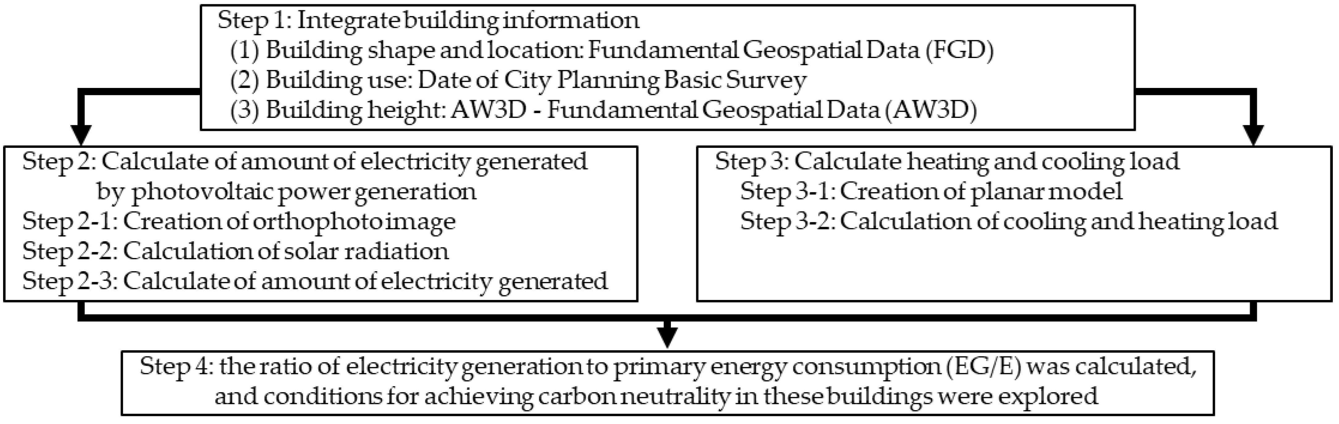
The procedure of this study was divided into four steps. Figure 1 shows an outline of the process.

STEP 1: GIS for the analysis was created from fundamental geospatial data (FGD), data of city planning basic survey (DCPBS), and an Advanced World 3D map (AW3D) [25,26,27].

STEP 2: The amount of electricity generated by the PV installed on walls was calculated with GIS (details of the work are described in Section 2.3). The process of calculating the amount of electricity generated on walls was further divided into three steps.

STEP 2-1: Building information was extracted from the created GIS data, and orthophoto images were created for each building (details of the work are described in Section 2.4).

STEP 2-2: The solar radiation obtained from AMeDAS was processed using orthophoto images to create solar radiation for each building (details of the work are described in Section 2.5).

STEP 2-3: The exterior wall surfaces where the PV would be installed were selected, and the amount of electricity generated at the wall surfaces was calculated from the solar radiation created (details of the work are described in Section 2.6).

STEP 3: The primary energy consumption of the buildings’ HVAC was calculated with the GIS. The process of calculating the primary energy consumption of the HVAC was further divided into two steps.

STEP 3-1: A calculation model was created for each building according to the input items of the calculation program for the primary energy consumption of air conditioning of buildings (details of the work are described in Section 2.7).

STEP 3-2: The primary energy consumption of the buildings’ HVAC was calculated with the calculation model (details of the work are described in Section 2.8).

STEP 4: The ratio of electricity generation to primary energy consumption (EG/E) was calculated, and conditions for achieving carbon neutrality in these buildings were explored (details of the work are described in Section 2.9). The amount of electricity generated was calculated in STEP 3. The primary energy consumption of the building is based on the $E_T$ entry in the BEI. BEI is the primary energy consumption of the designed building divided ($E_T$) by the primary energy consumption based on specified standard equipment specifications ($E_{ST}$). As aforementioned, in Japan, buildings are evaluated on the basis of a primary energy consumption index called BEI. BEI is expressed by the following Equations (1) and (2).

$$BEI=\frac{E_T}{E_{ST}}$$

(1)

$$E_T=E_{AC}+E_V+E_L+E_{SW}+E_{SEV}-E_s$$

(2)

The Energy Conservation Center, Japan (ECCJ) has surveyed energy consumption in office buildings [28]. Major energy-consuming equipment listed by the ECCJ is classified into the various items that make up $E_T$; $E_{AC}$ is the total energy consumption of heat source equipment, auxiliary equipment, water conveyance power, and air heat conveyance, $E_V$ is the energy consumption of ventilation, $E_L$ is the energy consumption of lighting, $E_{SW}$ is the total energy consumption of hot water supply, water supply, and drainage power, and $E_{SEV}$ is the energy consumption of elevators and escalators. The energy consumption of electrical outlets and other kinds of energy consumption are not included in the BEI. $E_{SW}$ and $E_{SEV}$ are 6–7% of the total energy consumption of an entire office building. Therefore, in this paper, the sum of $E_{AC}$, $E_V$, and $E_L$ was used as the energy consumption of an entire office building. $E_S$ is the amount of energy consumption reduced by improving the energy efficiency of facilities and the amount of electricity generated by PV.

R-language was used in this study. R-language is specialized in statistical and data analysis [29]. It can be installed free of charge from the web page of The Comprehensive R Archive Network. It can simplify the code for processing big data because it is capable of vector data processing. R-language has come into use with the processing of big data and the introduction of AI technology. All analyses in this study were performed in R-language except for Step3-2. GIS data in SHP file format can be analyzed in R-language.

An application featuring a simplified method for calculating heating and cooling loads (SKB47) was used to calculate the primary energy consumption. SKB47, which is provided by the Society of Heating, Air-Conditioning, and Sanitary Engineers of Japan (SHASE) [30], is an application that runs on Microsoft Excel, a Microsoft spreadsheet software program. The application can calculate the maximum heat load, annual heat load, annual primary energy consumption, and CO₂ emissions of air conditioning equipment once the calculation conditions are input. The input conditions for the calculations were limited to those that significantly impacted the heat load in an F-test during development. The application simplifies the calculation of the heat load. However, since there are model limitations when using it, the buildings were selected to match the limitations in the primary energy calculations described below.

2.3. Creation of GIS for Simulation

Building geometry and geographic information were obtained from three sources. The first was FGD provided by the Geospatial Information Authority of Japan (GSI) [25]. FGD has both GIS and digital elevation model (DEM) data. FGD’s GIS includes information on coastlines, road edges, and buildings. FGD’s DEM is mesh data on elevation that does not include the height of buildings and trees. This study used FGD’s GIS data surveyed in 2021–2022 and FGD’s DEM data surveyed in 2016–2018.

The second was the DCPBS provided by each municipality. DCPBS is data from periodic surveys conducted under the City Planning Act to determine the current status of cities and to plan for the future. DCPBS is GIS that combines geographic information with population size and the size of the working population by industry, urban area, land use, and traffic volume [26,31]. In this study, we obtained information on building use from DCPBS conducted by the city of Sapporo in 2011.

The third was AW3D, jointly provided by the NTT Data Corporation and the Remote Sensing Technology Center of Japan [27]. AW3D is produced by processing image data observed by the Advanced Land Observing Satellite (ALOS). AW3D’s DSM includes the heights of buildings and trees. In this study, AW3D created in 2015 was used.

Since FGD’s GIS is newer than DCPBS, building shapes were obtained from FGD’s GIS. However, building use details are not available from FGD’s GIS. When the center of gravity values of each building in FGD’s GIS and DCPBS were the same, the building uses from DCPBS were added to FGD’s GIS. Building heights cannot be obtained from FGD’s GIS and DCPBS. The elevation closest to the center of gravity of a building in FGD’s GIS was selected from AW3D’s DSM and FGD’s DEM, and the difference between the two elevations was added to FGD’s GIS as the height.

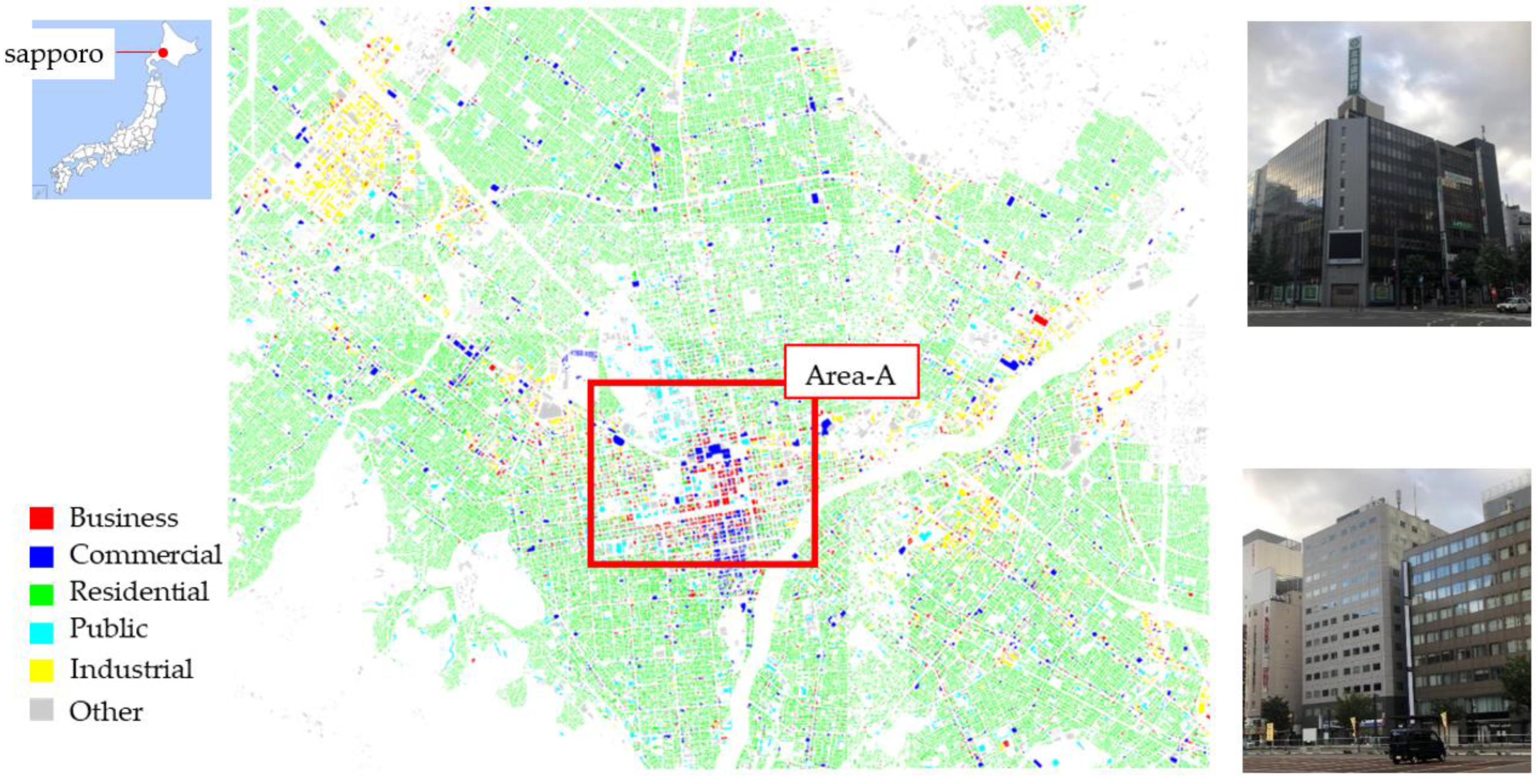
Figure 2 and

Table 2. Number of buildings.

	Business	Commercial	Residential	Public	Industrial	Other
Number	5062	3193	158,223	2679	3766	111,490

display a GIS created as maps classified by use. Buildings whose use could not be confirmed in the GIS were classified as other buildings. Residential buildings are widely distributed throughout Sapporo. Office buildings (BUSINESS), the target of this study, are also distributed throughout Sapporo, but the buildings with large building areas are densely located around Sapporo Station, the largest station in Sapporo. The area with the highest concentration of high-rise office buildings is designated as Area-A. Since Sapporo is a cold, snowy region, many office buildings have high thermal insulation and flat facades to prevent snow accumulation, as shown in the image in Figure 2.

2.4. Creation of Orthographic Images

To calculate the amount of electricity generated by PV installed on a wall, it is necessary to calculate the solar radiation, taking into account the surrounding shielding. By using an orthophoto image, meteorological data can be created that takes into account the effects of surrounding shielding. The sky view factor (SVF) can be calculated from the percentage of the sky in an orthophoto image. SVF is used as an indicator of the characteristics of urban geometry. Some papers have shown the relationship between the urban environment and SVF [32]. SVF is also used as a relevant indicator of both solar and ground radiation [33,34].

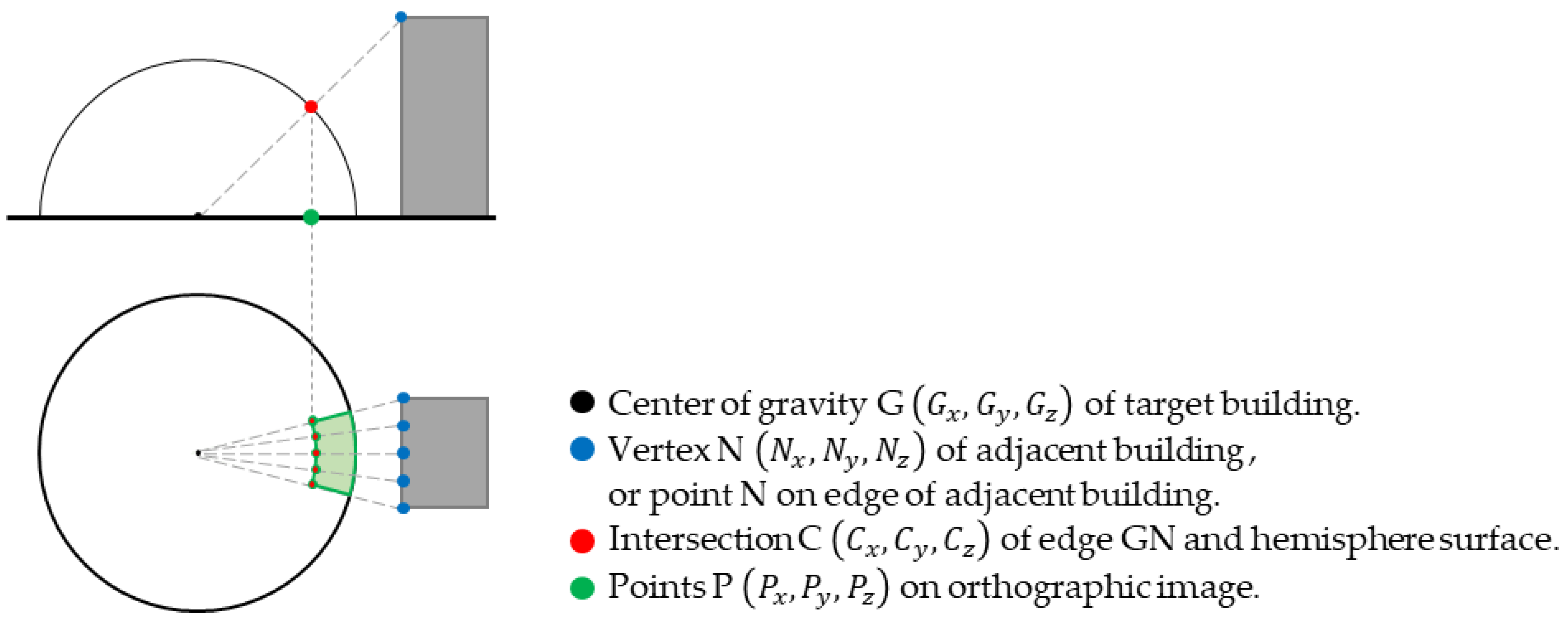
Buildings were selected from the GIS to create a positive projection image. These buildings are referred to as target buildings. In addition, from the GIS, buildings within a radius of 200 m around the center of gravity G of the target buildings were selected. The selected buildings are referred to as adjacent buildings. A hemisphere centered on the center of gravity G of a target building was assumed. Figure 3 shows the method of projecting the adjacent buildings onto an orthographic image. The bottom of the hemisphere is assumed to be an orthographic image. The black points in Figure 3 are assumed to be the center of gravity G $\left(G_x,G_y, G_z\right)$ of the target building. The blue points are the vertices N $\left(N_x,N_y,N_z\right)$ of the adjacent buildings or the points N on the edges. The red points are the points C $(C_x,C_y,C_z)$ on the hemispherical surface. Point C is the intersection of an edge GN and a hemisphere surface. It was calculated using the following Equation (3).

$$(C_x,C_y,C_z)=k\left(N_x-G_x,N_y-G_y,N_z-G_z\right)$$

(3)

k is a coefficient that converts a point on edge GN to a point on the surface of the hemisphere. k was calculated using the following Equation (4).

$$k=\frac{1}{\sqrt{{\left(N_x-G_x\right)}^2+{\left(N_y-G_Y\right)}^2+{\left(N_z-G_z\right)}^2}}$$

(4)

The green points in Figure 3 are the points P $(P_x,P_y,P_z)$ on the orthographic image. These points are projected from point C onto the positive projection image. Each point P was calculated by the following Equation (5).

$$(P_x,P_y,P_z)=\left(C_x,C_y,0\right)$$

(5)

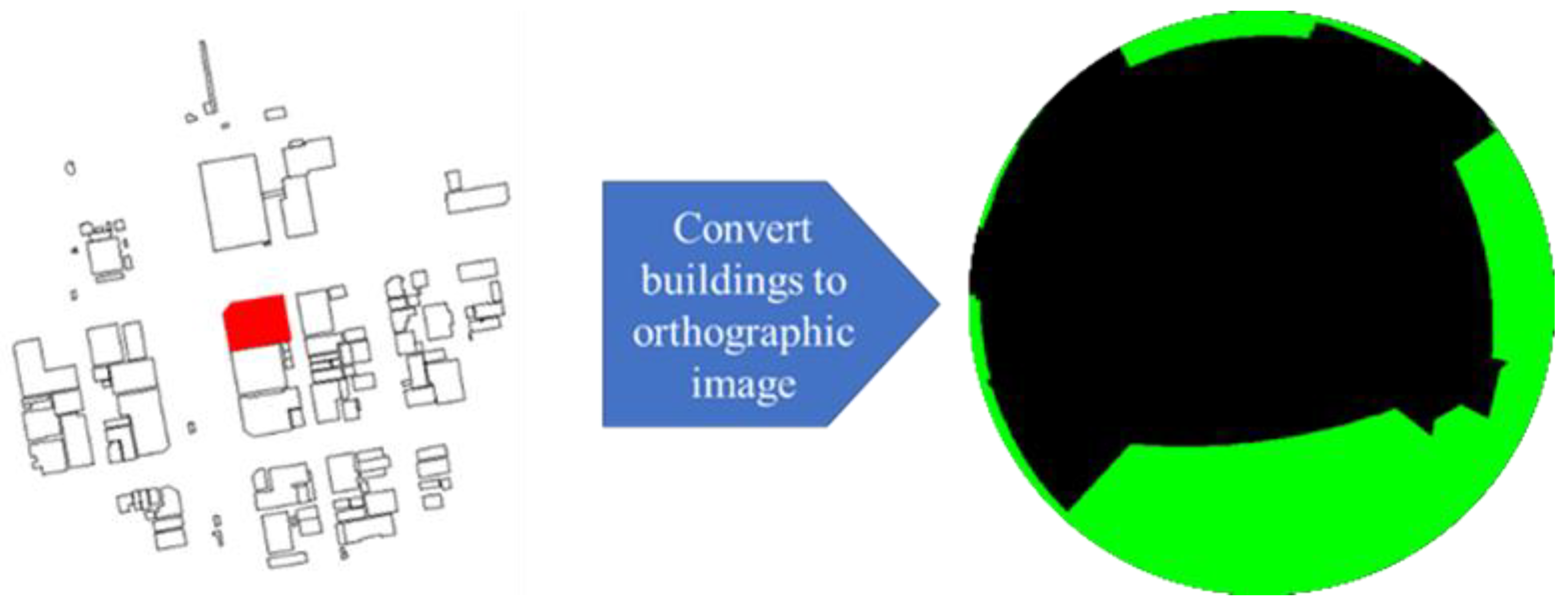
All points N of the adjacent buildings were projected onto the orthographic image by repeating Equations (3)–(5). The buildings were projected by filling in polygons composed of multiple points P projected onto the orthographic image. All adjacent buildings were projected in the same way. The orthographic image created is shown in Figure 4. The red building on the left is the target building, and the rest of the buildings are adjacent buildings. The right figure shows the result of converting the adjacent buildings around the target building into an orthographic image. SVF is the ratio of the sky area ($A_{sky}$) within the circle to the area of the circle ($A_{all}$). The SVF was calculated from the orthographic image using the following Equation (6).

$$SVF=\frac{A_{sky}}{A_{all}}$$

(6)

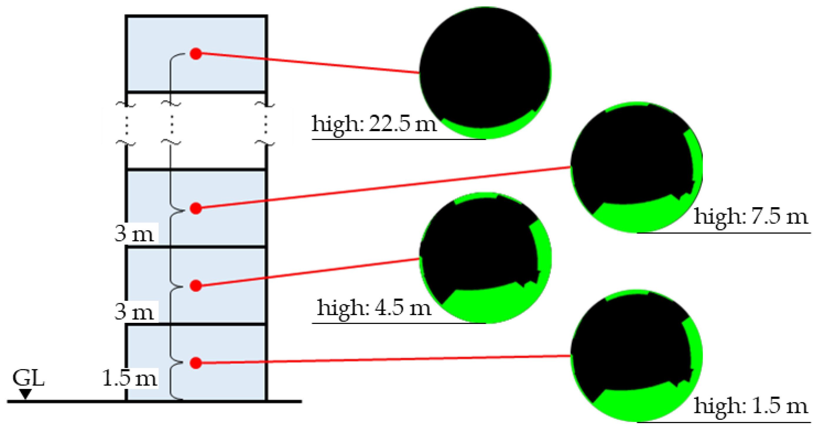
The influence of adjacent buildings varies depending on the height $G_z$ at which the orthographic image is created. Therefore, multiple orthographic images were created for a single building at different heights $G_z$ of the center of gravity. Figure 5 shows different height $G_z$ settings for the center of gravity and the orthographic images for each height. The lowest height was set at 1.5 m from the ground surface. From there, orthographic images were created for every 3 m in accordance with the height of the building. The images created for each height showed different shapes of adjacent buildings, indicating the need to create images for each height.

2.5. Calculation of Solar Radiation

The solar radiation ($I_{wall}$) incident on the wall surface is calculated from orthophoto images. Meteorological data were obtained from the Expanded AMeDAS Weather Data provided for a fee by the Meteorological Data System Co. in Kagoshima, Japan. The annual standard data is a hypothetical one-year data set created by selecting representative years by month from about 10 years of observation data and joining them. Observation data is measured by the Automated Weather Station (AWS) operated by the Japan Meteorological Agency [35]. These meteorological data have been used in other studies, and Akasaka et al. used these data to create climatic maps related to human thermal sensation [36]. In this paper, direct normal radiation ($I_{dire}$), diffuse horizontal radiation ($I_{diff}$), and outdoor temperature were obtained from the annual standard data of Expanded AMeDAS Weather Data from 2001 to 2010. The meteorological data were measured in an unobstructed environment. By using orthophoto images, $I_{dire}$ and $I_{diff}$ were reconstructed to $I_{wall}$ to account for the reduction in solar radiation due to adjacent buildings.

One exterior wall of the target buildings was selected, and the solar radiation obtained at that exterior wall was calculated. The orthophoto image created in Section 2.4 shows sky areas and adjacent buildings that are unnecessary for this calculation. Unnecessary areas were determined from the images in accordance with the orientation of the exterior walls. Figure 6 shows an orthographic image with the unnecessary areas filled in blue.

With an orthographic image, the diffuse radiation ($I_{wall-diff}$) and direct radiation ($I_{wall-dire}$) obtained at the exterior walls are calculated. The $I_{wall-diff}$ obtained at an exterior wall was calculated by $I_{diff}$ and SVF using the following Equation (7).

$$I_{wall-diff}=SVF·I_{diff}$$

(7)

The direct normal radiation not blocked by adjacent buildings was selected, and the direct normal radiation was converted in accordance with the orientation of the exterior walls. The hourly solar position was projected onto an orthographic image. If there was an adjacent building at the projected point, it was determined that direct normal radiation was not incident on the wall surface. The equation for calculating the solar position was based on the method proposed by Shinichi Matsumoto et al. [37,38,39,40,41]. Matsumoto et al. devised a more accurate and simpler equation for calculating the solar position on the basis of the Japan Coast Guard equation, which is highly accurate when calculating solar positions in Japan. The solar altitude (${\alpha }_{sun}$), solar azimuth angle (${\Phi }_{sun}$), and solar position were calculated in units of hours using the method of Matsumoto et al. The $I_{wall-dire}$ can be calculated from ${\alpha }_{sun}$, ${\Phi }_{sun}$, and the outward direction of the outer wall (${\Phi }_{wall}$). The $I_{wall-dire}$ was calculated using the following Equation (8).

$$I_{wall-dire}=c·I_{dire}·\sin {\alpha }_{sun}·\cos ({\Phi }_{sun}-{\Phi }_{wall})$$

(8)

When ${\alpha }_{sun}$ was less than 0°, $I_{wall-diff}$ and $I_{wall-dire}$ were set to 0 Wh/m². Since $I_{wall}$ is the sum of $I_{wall-dire}$ and $I_{wall-diff}$, it was calculated using the following Equation (9).

$$I_{wall}=I_{wall-dire}+I_{wall-diff}$$

(9)

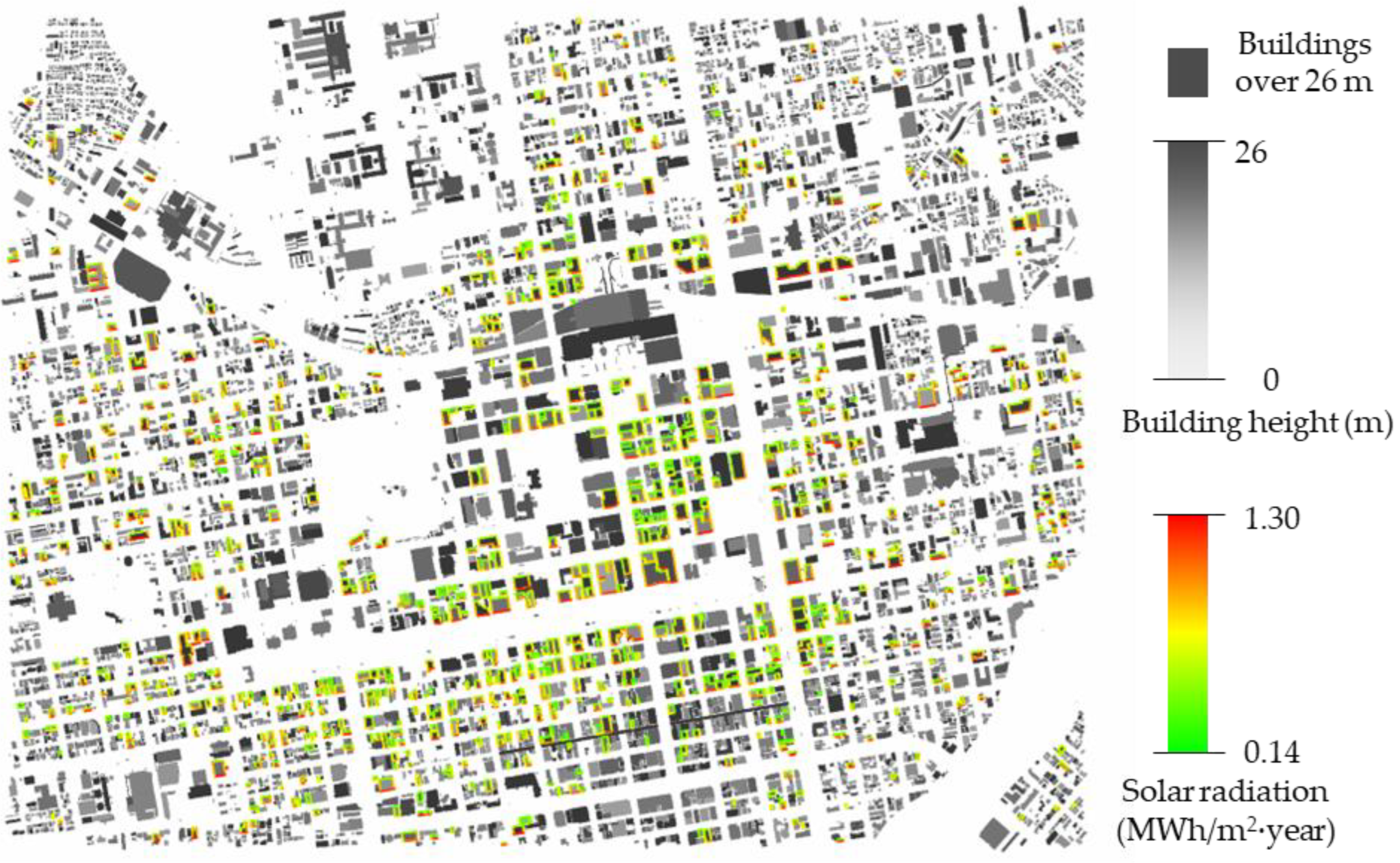
Figure 7 shows a distribution map using the results of calculating $I_{wall}$ in Area-A. As $I_{wall}$ increased, the color changed in the order of green, yellow, and red. The exterior walls in the south were mostly red. The exterior walls with adjacent buildings nearby turned green.

2.6. Calculation of Photovoltaic Electricity Generation

PV should not be installed on exterior walls where it would generate electricity inefficiently. If an adjacent building is in the immediate vicinity of an exterior wall, there is a risk that the solar radiation obtained will be small. Therefore, we decided that exterior walls that meet the following two criteria should not have PV panels installed on them.

(1) If building is within 4 m of exterior wall: if there is an adjacent building near an exterior wall, the generated electricity will be drastically reduced because the adjacent building will block much of the solar radiation. Article 42 of The Building Standard Law of Japan states that the minimum distance for the width of a road is 4 m [42]. If an adjacent building is within 4 m of an exterior wall, the wall is defined as a wall where PV cannot be installed.

(2) If exterior wall is less than 3 m wide: if the exterior wall is less than 3 m wide, it is likely to be part of a curved surface or the side of an area projecting outdoors. Both conditions were defined as exterior walls where PV could not be installed due to structural problems with the PV panels and problems obtaining sufficient solar radiation.

The amount of electricity generated by PV was calculated from the solar radiation on each wall in Section 2.5. Calculations were made by dividing each wall surface by 3 m in the height direction. The formula of JISC8907 was used to calculate the amount of electricity generated [43]. The electricity generated was calculated as the product of the amount of electricity generated per unit area and the exterior wall surface area. However, the amount of electricity generated for exterior walls that met conditions (1) and (2) above was set to 0 kWh/(m²·year). The electricity generated for a building ($E{G}_{build}$) was calculated using the following Equations (10) and (11).

$$E{G}_{wall}=W_{wall}({\displaystyle \sum }_i^{N_{SVF}}E{G}_{high}\left(i\right)·3+E{G}_{high}\left(N_{SVF}\right)·\left(H_{build}-3·N_{SVF}\right))$$

(10)

$$E{G}_{build}={\displaystyle \sum }_i^{N_{wall}}E{G}_{wall}\left(i\right)$$

(11)

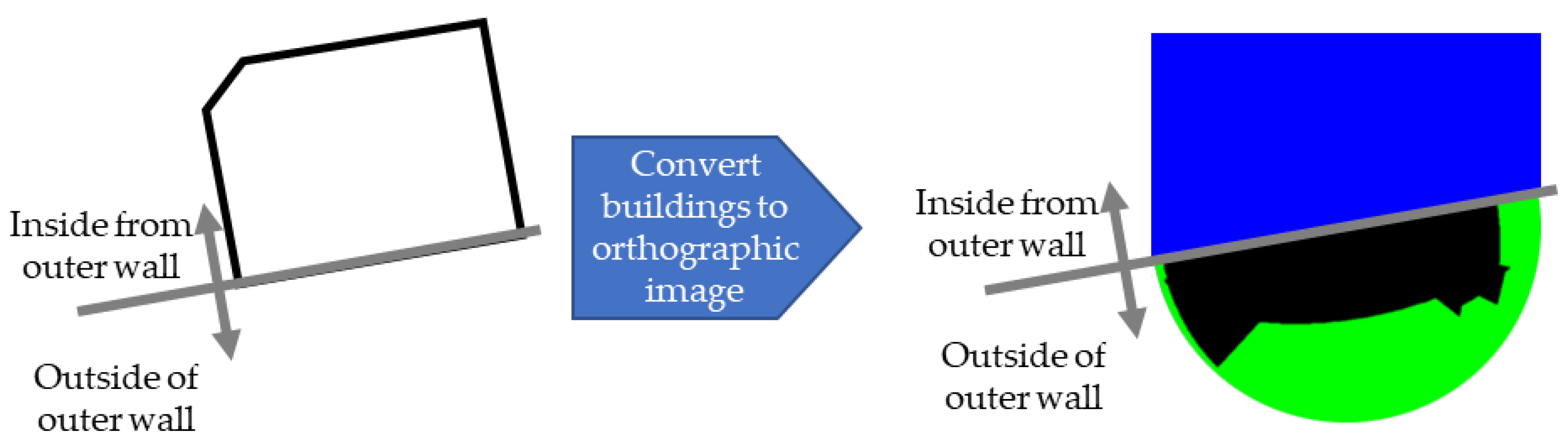
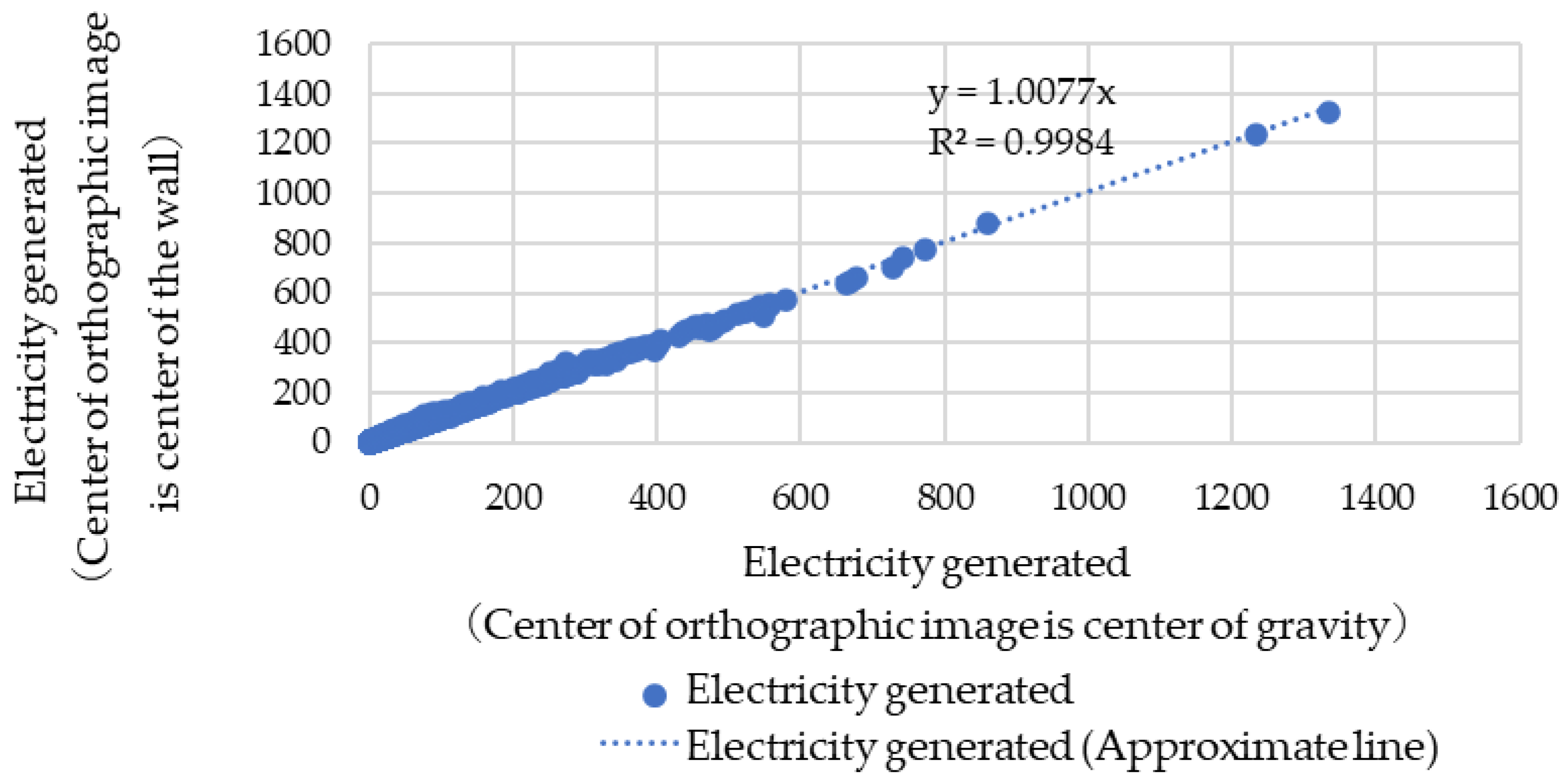
When different orthoimages were created for the same building at different locations, we checked how the differences affected the amount of electricity generated. Suppose there is a building in front of a wall. There may be an error in electricity generation between the orthographic image at the gravity center and that at the wall center. However, in this paper, the above conditions (1) and (2) exclude exterior walls with adjacent buildings that would significantly affect the electricity generated on the wall surface, and thus, the error is small. Figure 8 shows a comparison of the electricity generation of a building in an orthographic image at the gravity center and at the wall center. The data targets 3539 target buildings. Pearson’s product-rate correlation coefficient was used to analyze the two sets of data. Pearson’s product-moment correlation coefficient allows one to analyze the similarity of two sets of data. Since the results for both were almost identical, it indicated that there was little error between the two.

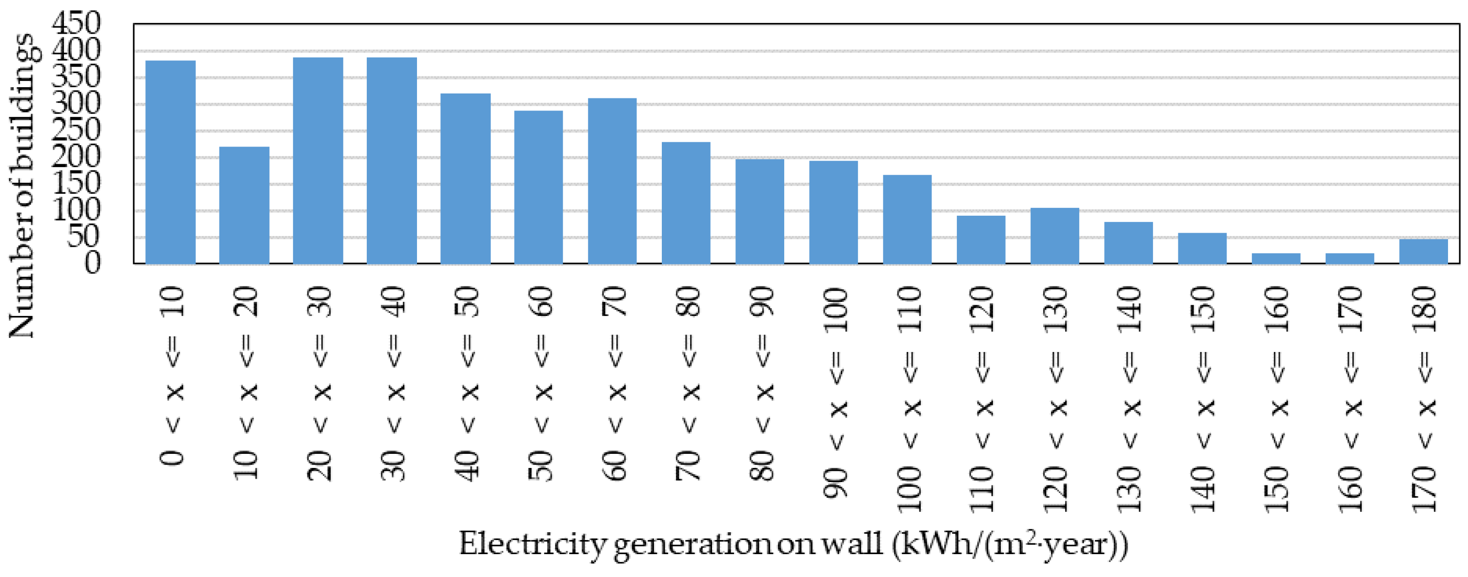
Figure 9 shows a histogram of the annual electricity generation. Many buildings had electricity generation ranging from 0 kWh/(m²·year) to 40 kWh/(m²·year). Some buildings generated 170 kWh/(m²·year) to 180 kWh/(m²·year), depending on the location.

2.7. Model for Primary Energy Consumption

The calculation of the primary energy consumption with SKB47 requires the parameters shown in

Table 3. Room conditions.

Parameter			Unit
Indoor temperature setting	Cooling	26	degree
	Heating	22	degree
Internal heating	Lighting capacity	10	W/m2
	Outlet capacity	15	W/m2
	Number of occupants	0.1	Person/m2
Air conditioning	Heating preheat time	1	Hour
	Amount of outdoor air	5	m3/(m2·h)
	Total heat exchanger efficiency	70	%
Air conditioning equipment	PAC (Annual Performance Factor)	5	-

for each zone. The shape of the interior zones and the perimeter zones were calculated from building outlines. The required calculation conditions for each zone are shown in

Table 4. Calculation conditions.

Item	Input
Number of floors	Number of floors (-)
Floor type	Top floor or Middle floor (-)
Outward orientation of exterior wall with largest windows	Azimuth (°)
Type of zone	Interior zone or Perimeter zone (-)
Floor area of zone	Number (m2)
Percentage of window area to exterior wall	Number (%)
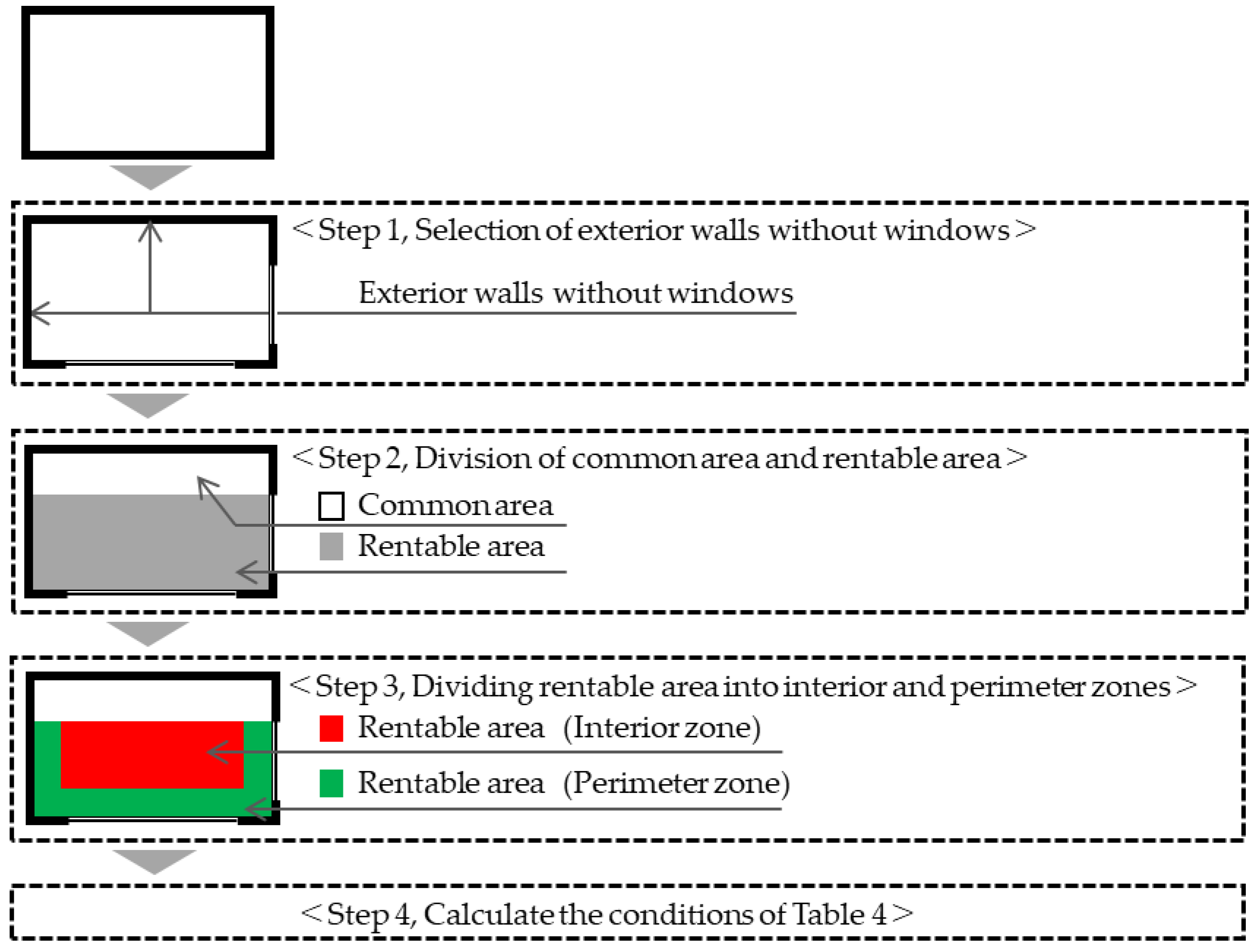
Room depth	Floor area/Exterior wall width (m)

. The flow diagram of the computational modeling procedure is shown in Figure 10. Many buildings in Sapporo have simple facades, as shown in Figure 2, due to the large amount of snowfall. The facade of the model was a flat plane with no eaves or balconies.

The procedure for creating the calculation model from building outlines is as follows.

Step 1. Selection of exterior walls without windows: exterior walls without windows were determined from the outlines of the target buildings. Since the size of a window affects the heating and cooling load, it is necessary to consider whether to install a window on an exterior wall. Suppose there is an adjacent building in the immediate vicinity of an exterior wall. In that case, it would be likely that the installation of windows on that wall would be abandoned during the design phase. Therefore, the conditions for exterior walls where no windows are to be installed are the same as those for not installing PV in Section 2.6.

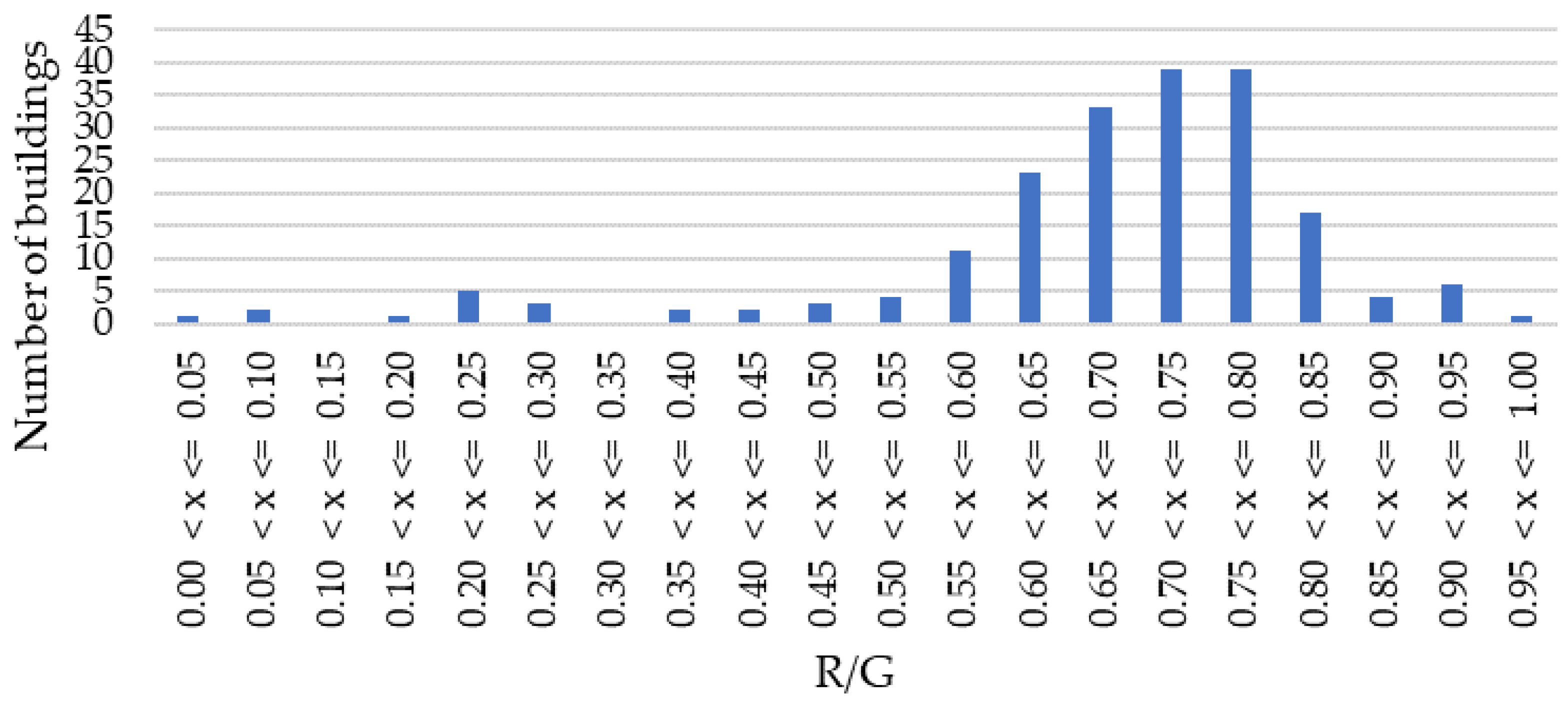
Step 2. Division of common area and rentable area: from building outlines, the building plans were divided into a common area and a rentable area. The exterior wall with the longest width was selected from among the exterior walls where windows could be installed, and an interior wall parallel to the exterior wall was created. The polygonal shape, including the exterior wall, was designated as a rentable area, and the remainder was designated as a common area. In Japan, rentable area divided by gross floor area is used as an indicator of a building’s profitability. In this paper, this index is referred to as R/G. The characteristics of the R/G of Japanese office buildings were confirmed from IR information on Japanese investment corporations [44,45,46,47,48]. IR information allows commercial companies to publicly disclose their business and financial conditions, and information on real estate owned by the company can be obtained from IR information. Figure 11 shows a histogram of R/G. When only office buildings were selected from the IR information, the total number of cases was 196. The range of R/G with the highest number of office buildings was from 70% to 75% and from 75% to 80%. Therefore, the calculation model was created so that the leased area would be between 70% and 75%.

Step 3. Dividing rentable area into interior and perimeter zones: a line was drawn inside the rentable area, 5 m away from the exterior wall, and the area consisting of the exterior wall and the line was designated as the perimeter zone, while another area was designated as the interior zone. The model created divides the plane into three areas, as in the model represented in step 3 of Figure 10. The colorless area is the common area, the red is the interior zone, and the green is the perimeter zone.

Step 4. Calculate the conditions of Table 4: the number of floors was entered by dividing the building height by 4 m. The top floor was entered as the uppermost floor, and the middle floor was entered as the remaining floor. For the exterior orientation of the exterior wall with the largest window, the orientation of the exterior wall with the smallest width, where the window selected in Step 2 could be installed, was entered. The zone type and area were entered by using the results of Step 3. Three cases of window area were assumed: 25%, 50%, and 75% of the exterior wall on which a window could be installed. The window-to-exterior-wall ratio was entered as the ratio of window area to the total exterior wall area of the rentable area. The room depth was entered as the floor area of the rentable area divided by the width of all exterior walls of the rentable area.

2.8. Calculation of HVAC Primary Energy Consumption

The primary energy consumption ($E_{AC}+E_V$) for HVAC was calculated using SKB47. The SKB47 model requires at least 6 m as the room depth. Four hundred and fifteen buildings with an R/G of 70–75%, which were selected from among all office buildings in Sapporo, were calculated. In calculating $E_{AC}+E_V$, a parametric study was conducted on the thermal transmittance of the exterior ($U_{wall}$) walls and the thermal transmittance of the windows ($U_{window}$) and window area ($A_{window}$). For the exterior walls, the thermal transmittance was set for three cases with insulation thicknesses of 50 mm, 100 mm, and 200 mm.

Table 5. Exterior wall model.

	Heat Transmission Coefficient (W/(m2·K))
OW1	0.1792
OW2	0.3391
OW3	0.6122

shows the thermal transmittance of each exterior wall. A total of four cases were examined: two cases for the window type and two cases with and without blinds.

Table 6. Window model.

	Type	Blind	Heat Transmission Coefficient (W/m2·K)	Shading Coefficient
WQ1	Triple glazing	ON	1.0	0.136
WQ2	Triple glazing	OFF	1.3	0.409
WQ3	Double glazing	ON	2.2	0.470
WQ4	Double glazing	OFF	2.6	0.690

shows case studies for each window model. The sizes of the windows are 25%, 50%, and 75% of the area of the exterior wall ($A_{wall-rent-window}$) that is adjacent to the rentable area and where the windows can be installed.

Table 7. Window area sizes.

	${\mathit{A}}_{\mathit{w}\mathit{i}\mathit{n}\mathit{d}\mathit{o}\mathit{w}}$$/{\mathit{A}}_{\mathit{w}\mathit{a}\mathit{l}\mathit{l}-\mathit{r}\mathit{e}\mathit{n}\mathit{t}-\mathit{w}\mathit{i}\mathit{n}\mathit{d}\mathit{o}\mathit{w}}(\%)$
Case-1	25
Case-2	50
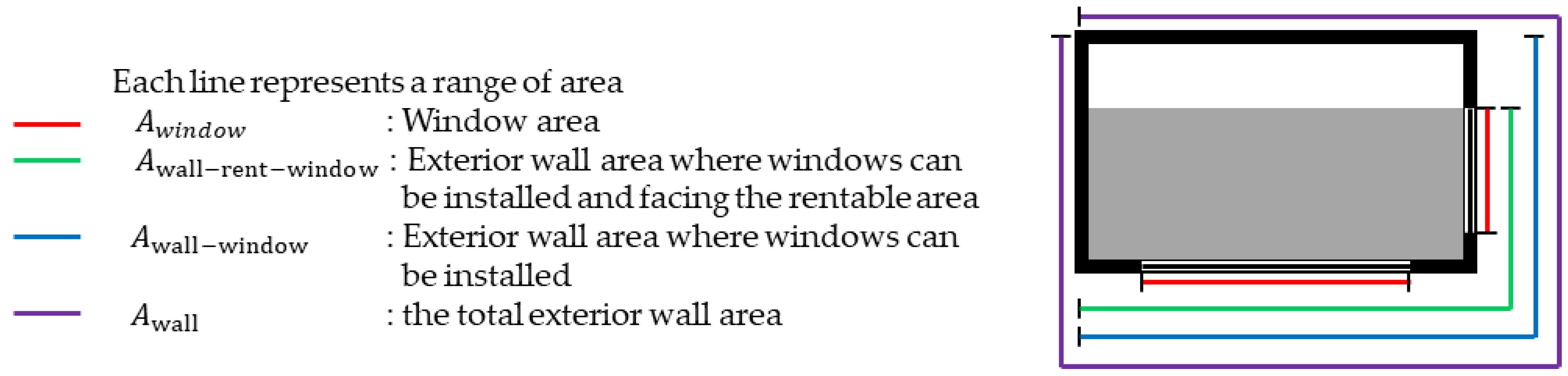
Case-3	75

shows the window area sizes. The PV area is the area of all exterior walls where windows can be installed ($A_{wall-window}$) minus $A_{window}$. $A_{wall-window}$ is the area of the exterior wall that can be installed with the windows selected in STEP1 of Section 2.7. Figure 12 shows the respective ranges of $A_{window}$, $A_{window-rent-window}$, $A_{wall-window}$ and $A_{wall}$. The calculations were performed for 36 cases per building.

2.9. Calculating Electricity Generation as Percentage of Primary Energy Consumption

The amount of electricity generated ($EG/E$) relative to the primary energy consumption of the buildings was calculated. When $EG/E$ is 1, CO₂ emissions are virtually zero, indicating that carbon neutrality has been achieved. $EG/E$ was calculated using the following Equations (12)–(14).

$$EG/E=\frac{E{G}_{build}}{E_{build}}$$

(12)

$$E_{build}=\frac{\left(E_{AC}+E_V+E_L\right)}{3600}$$

(13)

$$E_L=9.97\left(Q_L·h{r}_L·dy·A_{build}\right)$$

(14)

$E{G}_{build}$ is a building’s generated electricity calculated as in Section 2.6. $E_{build}$ is the energy consumption of an entire office building. This value is the sum of the primary energy consumption of air conditioning ($E_{AC}$), ventilation ($E_V$), and lighting ($E_L$), which are organized from the energy consumption section of the BEI in Section 2.2. $E_L$ is the primary energy consumption of lighting. The electricity consumption of lighting ($Q_L$) was assumed to be equal to the internal heat generation of the lighting. The operating hours of lighting ($h{r}_L$) were assumed to be from 8:00 to 21:00 on weekdays, the same as the operating hours of the air conditioning. The number of weekday days in Japan ($dy$) was set to 245. These values were multiplied by the lighting’s primary energy conversion factor of 9.97 MJ/kWh to obtain the primary energy consumption of lighting ($E_L$) [49]. $EG/E$ was calculated for 36 cases per building. Since there were 415 buildings, a total of 14,940 calculations were performed.

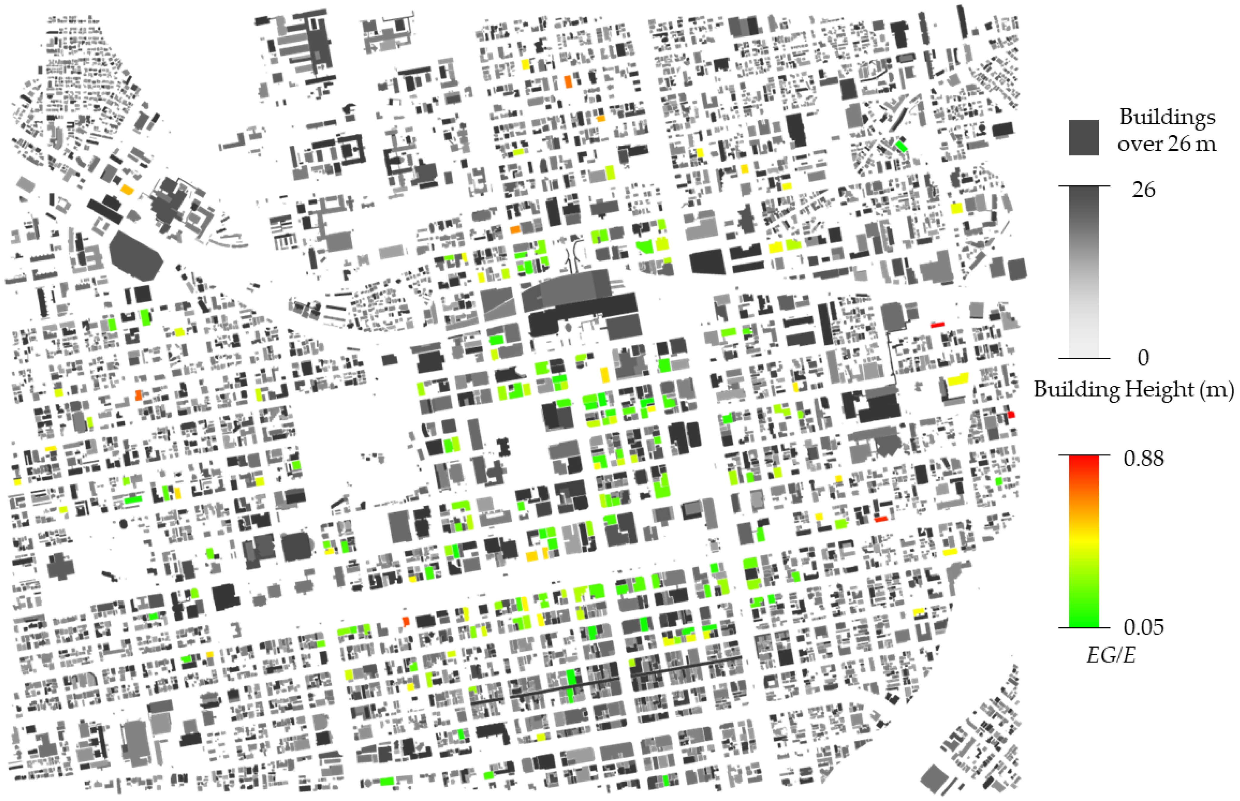
Figure 13 shows the distribution of $EG/E$ calculation results for Area-A with OW1 as the exterior wall model, WQ1 as the window model, and Case-1 as the window area type. Since Area-A is an area with a high concentration of tall buildings, the $EG/E$ of many buildings was green to yellow. The $EG/E$ of buildings with open south sides was mostly red. However, the $EG/E$ of a few buildings was green or yellow, despite the buildings having an open south side. The large difference in $EG/E$ among office buildings in similar surroundings was due to the shape and performance of the buildings themselves; some buildings outside of Area-A had a $EG/E$ greater than 1.

3. Result and Discussion

A multiple regression analysis of $EG/E$, electricity generation ($E{G}_{build}$), and $E_{build}$ was performed. The appropriate sample size for multiple regression analysis was determined by entering the critical values (α), power (1 − β), explanatory variables, and effect size (f ²) into G * power. G * Power is a free software program that can determine the optimal sample size depending on the analysis method. When the critical values were set at 1%, power at 99%, explanatory variables at 11, and effect size at 15% in this paper, an appropriate sample size of 287 cases was calculated. We extracted 287 cases from the 14,940 calculated results. There are no identical buildings in the 287 cases extracted, and the conditions for a total of 36 cases listed in Table 5, Table 6 and Table 7 are also not skewed. Multiple regression analysis can create predictive equations for the objective variable using explanatory variables, and by calculating the standard regression coefficient for each value, the relationship between the objective variable and each explanatory variable can be analyzed. There were 11 explanatory variables, which were divided into 3 groups. The first group represented building performance. This group assumed three explanatory variables: thermal transmittance of windows ($U_{window}$), solar shading coefficient of windows ($S{C}_{window}$), and thermal transmittance of exterior walls ($U_{wall}$). The second group represented building shape. This group assumed four explanatory variables: building area ($A_{floor}$), value obtained by dividing the PV area by $A_{wall}$ ($A{P}_{PV}$), value obtained by dividing $A_{window}$ by $A_{wall}$ ($A{P}_{window}$), and building height ($H_{build}$). $A_{wall}$ is the area of all exterior walls of the building. $A{P}_{window}$ and $A{P}_{PV}$ are different from the window area sizes in Table 7. The window area sizes in Table 7 are the values obtained by dividing $A_{window}$ by $A_{window-rent-window}$. 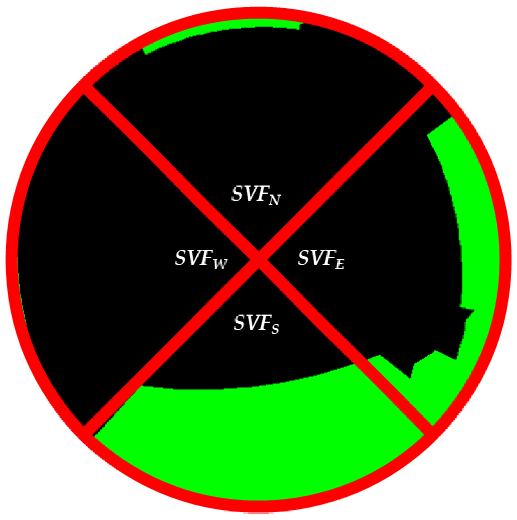The difference between $A_{window}$, $A_{window-rent-window}$ and $A_{wall}$ is shown in Figure 12 in Section 2.8. The third group represented the external environment. This group assumed four explanatory variables with the sky coverage broken down into $SV{F}_N$, $SV{F}_W$, $SV{F}_S$, and $SV{F}_E$. The SVF from northeast to northwest was assumed to be $SV{F}_N$, from northwest to southwest $SV{F}_W$, from southwest to southeast $SV{F}_S$, and from southeast to northeast $SV{F}_E$. Figure 14 shows an imaginary diagram of the four $SVF$. The VIFs of the explanatory variables were all less than 10, so there was no multicollinearity.

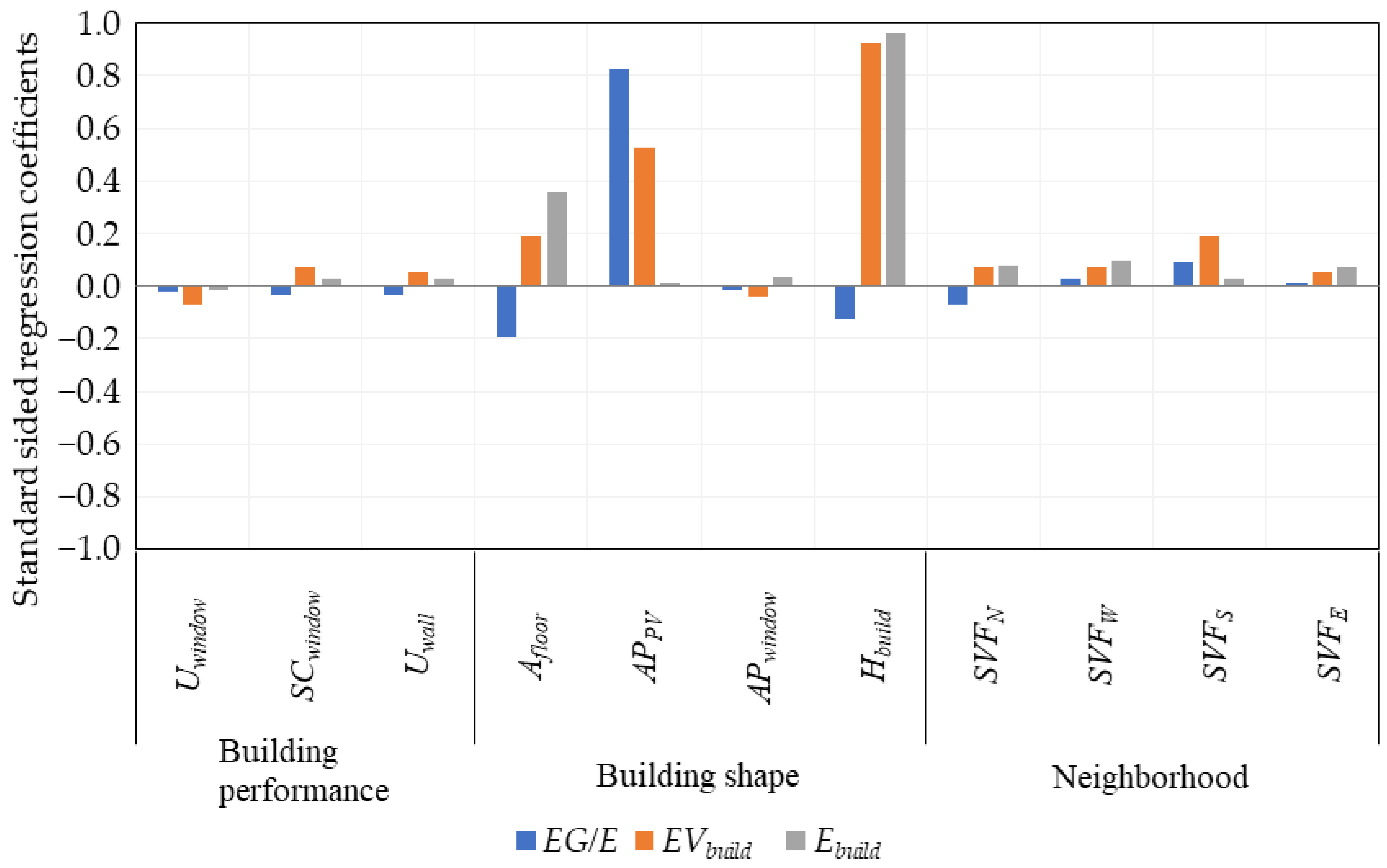
The results of the multiple regression analysis are shown in

Table 8. Results of multiple regression analysis.

Analysis Result of $E_{build}$
	Building Performance			Building Shape				Neighborhood
	$U_{window}$	$S{C}_{window}$	$U_{wall}$	$A_{floor}$	$A{P}_{PV}$	$A{P}_{window}$	$H_{build}$	$SV{F}_N$	$SV{F}_W$	$SV{F}_S$	$SV{F}_E$
Standardized partial regression coefficient	−0.011	0.026	0.032	0.359	0.013	0.035	0.961	0.076	0.097	0.028	0.074
p-value	0.809	0.579	0.101	0.000	0.523	0.083	0.000	0.005	0.001	0.264	0.005
Analysis Result of $E{G}_{build}$
	Building Performance			Building Shape				Neighborhood
	$U_{window}$	$S{C}_{window}$	$U_{wall}$	$A_{floor}$	$A{P}_{PV}$	$A{P}_{window}$	$H_{build}$	$SV{F}_N$	$SV{F}_W$	$SV{F}_S$	$SV{F}_E$
Standardized partial regression coefficient	−0.069	0.071	0.054	0.193	0.525	−0.039	0.921	0.074	0.071	0.194	0.052
p-value	0.266	0.255	0.035	0.000	0.000	0.133	0.000	0.036	0.054	0.000	0.136
Analysis Result of $EG/E$
	Building Performance			Building Shape				Neighborhood
	$U_{window}$	$S{C}_{window}$	$U_{wall}$	$A_{floor}$	$A{P}_{PV}$	$A{P}_{window}$	$H_{build}$	$SV{F}_N$	$SV{F}_W$	$SV{F}_S$	$SV{F}_E$
Standardized partial regression coefficient	−0.020	−0.030	−0.030	−0.196	0.826	−0.017	−0.126	−0.070	0.028	0.091	0.011
p-value	0.727	0.604	0.203	0.000	0.000	0.494	0.002	0.035	0.412	0.004	0.723

and Figure 15. Although many studies indicated that building performance and neighborhood affect the energy consumption of a building and the amount of electricity generated by wall-mounted PV [50,51,52,53,54], the results of this study indicate that building shape has the greatest impact on each of the objective variables. In general, building performance has a large effect on the objective variables, but in this analysis, the effects were small because only those with good building performance were included. $E_{build}$ is significantly different from $A_{floor}$, $H_{build}$, $SV{F}_N$, $SV{F}_W$, and $SV{F}_E$ with p-values less than 0.05. Building performance has an impact on the HVAC primary energy consumption, but its share of $E_{build}$ was small, so it was not significantly different. Explanatory variables of the significant difference for $E_{build}$ were positively correlated. The effect size of H_build was considerable. $E{G}_{build}$ is significantly different from $U_{wall}$, $A_{floor}$, $A_{PV}$, $H_{build}$, $SV{F}_N$, $SV{F}_S$, and $SV{F}_E$ with p-values less than 0.05. $E{G}_{build}$ was positively correlated with $A_{floor}$, $A{P}_{PV}$, and $H_{build}$, which are factors that increase the PV area. $E{G}_{build}$ was positively correlated with all explanatory variables of the external environment, which are factors that increase the solar radiation that can be obtained. $EG/E$ is significantly different from $A_{floor}$, $A_{PV}$, $H_{build}$, $SV{F}_N$, and $SV{F}_S$ with p-values less than 0.05. The $A{P}_{PV}$ for building shape concerning $EG/E$ showed a positive correlation, while $A_{floor}$ and H_wall showed a negative correlation. $SV{F}_S$ for the external environment for $EG/E$ showed positive correlations, while $SV{F}_N$ showed negative correlations. Since $EG/E$ is the value obtained by dividing $E{G}_{build}$ by $E_{build}$, the regression coefficient of each explanatory variable for $EG/E$ changed positively or negatively depending on the amount of effect of each explanatory variable for $E{G}_{build}$ and $E_{build}$. The positives and negatives of the regression coefficients of each explanatory variable on $EG/E$ changed.

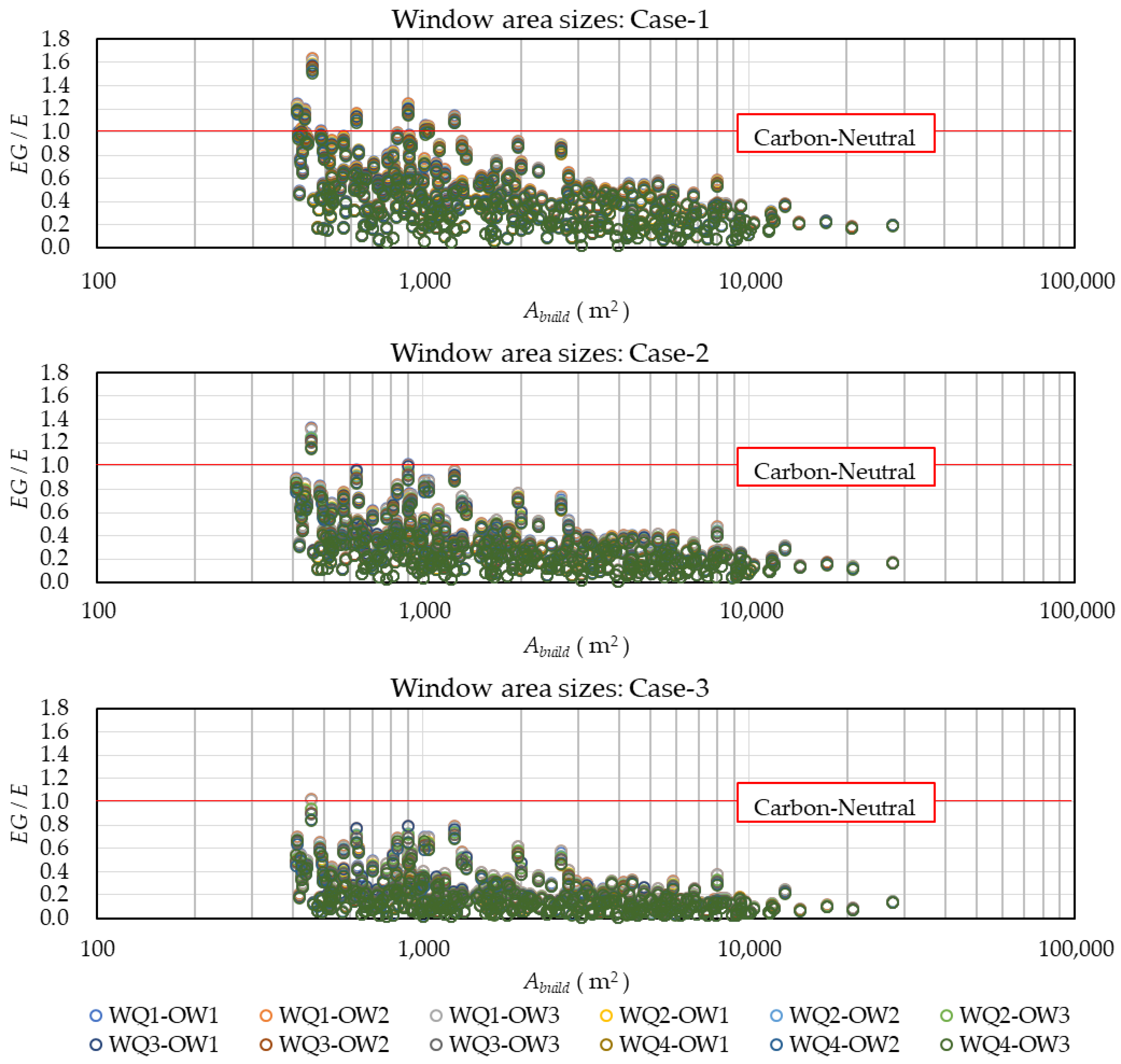
Scatter plots of $EG/E$ against the gross floor area ($A_{build}$) are shown in Figure 16. Three figures in Figure 16 are displayed for each window area size shown in Table 7. The color of the plots was different for each window and exterior wall performance. The maximum fluctuation of $EG/E$ due to differences in the window and exterior wall performance was about 0.13. However, as the gross floor area increased, the fluctuation of $EG/E$ due to these differences disappeared. The fluctuations in $EG/E$ due to changes in the percentage of window area were significant. The below studies indicate that a smaller percentage of window area is advantageous in reducing heating and cooling loads [55,56,57,58]. Comparing Cases 1, 2, and 3 in this analysis, Case 1, which has a smaller window area, had a larger EG/E due to a smaller heating/cooling load and was closer to carbon neutrality. In all cases, there were buildings where $EG/E$ exceeded 1. The smaller the window area ratio, the greater the $EG/E$ value because the heating and cooling loads were reduced, and the PV area was increased. It was shown that for buildings with a small gross floor area, improving the performance of windows and exterior walls and providing a larger PV area would result in a $EG/E$ above 1, indicating that carbon neutrality for such buildings can be achieved. However, for buildings with a large gross floor area, it is difficult to improve $EG/E$ by improving the performance of windows and exterior walls or by increasing the PV area. Therefore, to improve $EG/E$, it is necessary to use equipment with higher performance and consider more efficient operation for HVAC systems.

4. Conclusions

One of the major challenges is achieving carbon neutrality in buildings. PV can make a significant contribution to achieving carbon neutrality. However, to determine the electricity generated by PV, it is necessary to conduct a PV simulation that considers a city’s shape. Although GIS has facilitated the modeling of cities, simulating PV in a 3D model with multiple buildings is still computationally demanding. In this study, we proposed a method for representing the complex geometry of a city in 2D images and simulating the amount of electricity generated by PV using these images over a short period of time and in large quantities. We also calculated the electricity generation ratio to primary energy consumption ($EG/E$) for each building and explored conditions for achieving carbon neutrality in buildings.

(1) The GIS used in this methodology was created using FGD, DCPBS, and AW3D. It was confirmed that office buildings are distributed throughout Sapporo, but buildings with large building areas are concentrated around Sapporo Station, the largest station in Sapporo.

(2) An orthographic image was created from the GIS. Solar radiation was calculated using this image, taking into account the effects of surrounding shielding. The conditions for an exterior wall to obtain a large amount of solar radiation were confirmed to be that the exterior wall faces south and that there are no adjacent buildings in the vicinity of the exterior wall. The electricity generated was calculated from the calculated solar radiation. Many office buildings in Sapporo generate 0 kWh/(m²·year) to 40 kWh/(m²·year). It was confirmed that the generation of 170 kWh/(m²·year) to 180 kWh/(m²·year) can be expected depending on the location.

(3) Models of buildings were created from the GIS, and the primary energy consumption of the buildings was calculated. The electricity generated ($EG/E$) relative to the primary energy consumption of the buildings was also calculated. Some buildings in Area-A had significantly different $EG/E$, even for office buildings in similar environments, depending on the shape and performance of the buildings themselves. Some of the buildings calculated had a $EG/E$ greater than 1.

(4) A multiple regression analysis was performed for $EG/E$, $E_{build}$, and $E{G}_{build}$ using 11 explanatory variables. It was shown that for buildings with a small gross floor area, improving the performance of windows and exterior walls and ensuring a large PV area would result in a $EG/E$ of higher than 1, indicating that carbon neutrality can be achieved. However, for buildings with a large gross floor area, it is difficult to improve $EG/E$ by improving the performance of windows and exterior walls or by having a large PV area. Therefore, to improve $EG/E$, it is necessary to consider improving the performance of the equipment used and the efficient operation of HVAC systems.

The results in this paper are based on the assumption that the climatic conditions are those of Sapporo. However, the proposed method can be used in any city where GIS data is available. In addition, a large number of buildings can be simulated in a short amount of time using this method. This method is useful for studying the introduction of PV to new cities and the carbon neutrality of buildings.

5. Limitations and Future Work

Limitations of this study and prospects for future research are described below.

(1) Addition of radiance distribution: this paper did not consider radiance distribution. In addition, when it comes to wall surfaces, reflections from the ground and buildings must also be taken into account. In the future, we will consider a method that enables simple calculations while including the effects of radiance distribution and reflections by expressing the distance to a building in an orthographic image.

(2) Consideration of influence of trees: it was possible that the difference in elevation between AW3D’s DSM and FGD’s DEM was due to trees in areas where there are no buildings in the GIS. However, when the locations of trees were confirmed from a hollow photograph of Sapporo provided by FGD, the trees were not present at the assumed tree locations in the photograph. The resolution of FGD’s DEM is 5 m. Therefore, when the distance between trees and buildings was less than 5 m, trees were determined to be located on the part of the ground between the trees and buildings. In the future, a method for accurately determining the locations of trees and reflecting them in orthographic images will be investigated.

(3) Simulation of primary energy consumption by Energy Plus: in this study, SKB47 was used to calculate the primary energy consumption of buildings. SKB47 was able to calculate the primary energy consumption of many buildings in a short period of time by simplifying the heat load calculation. However, the number of buildings that could be used for heat load calculations was limited. In addition, the solar radiation data used ignored the effects of urban geometry. In actual office operations, when solar radiation is high, openings are temporarily closed due to glare, but the operation of these openings was not included in the calculations. In the future, Energy Plus will be used for heat load calculations [59]. This software can use the solar radiation calculated by this method, and the operation of the openings can be reflected in the calculation results. It is also possible to calculate the heat load of a building, which was not possible with SKB47. By using the calculation results from Energy Plus, more elaborate studies can be performed.