Open-Circuit Voltage Models for Battery Management Systems: A Review

Abstract

A battery management system (BMS) plays a crucial role to ensure the safety, efficiency, and reliability of a rechargeable Li-ion battery pack. State of charge (SOC) estimation is an important operation within a BMS. Estimated SOC is required in several BMS operations, such as remaining power and mileage estimation, battery capacity estimation, charge termination, and cell balancing. The open-circuit voltage (OCV) look-up-based SOC estimation approach is widely used in battery management systems. For OCV lookup, the OCV–SOC characteristic is empirically measured and parameterized a priori. The literature shows numerous OCV–SOC models and approaches to characterize them and use them in SOC estimation. However, the selection of an OCV–SOC model must consider several factors: (i) Modeling errors due to approximations, age/temperature effects, and cell-to-cell variations; (ii) Likelihood and severity of errors when the OCV–SOC parameters are rounded; (iii) Computing system requirements to store and process OCV parameters; and (iv) The required computational complexity of real-time OCV lookup algorithms. This paper presents a review of existing OCV–SOC models and proposes a systematic approach to select a suitable OCV–SOC for implementation based on various constraints faced by a BMS designer in practical application.

1. Introduction

Li-ion batteries first entered the commercial market as portable batteries for consumer electronics. Today, the use of battery-operated rechargeable systems is envisioned to be the most promising alternative for hazardous emissions due to the use of fossil fuels [1]. Moreover, passenger electric vehicles will continue to see the dominant use of Li-ion batteries [2]. In recent times, it has become customary to constantly monitor and manage a battery using a battery management system (BMS) [3] to ensures the safe, efficient, and reliable operation of the battery. BMSs are usually made of the following three components: a battery fuel gauge (BFG), an optimal charging algorithm (OCA), and cell balancing circuitry (CBC). The BFG is the most important element of a BMS, and it estimates several important states and parameters of the battery, including the state of charge (SOC). The CBC ensures safety by preventing cell imbalance between batteries in a battery pack. The OCA allows faster charging during usage without affecting the battery’s health. It is important to note that accurate SOC estimation by the BFG is crucial for efficient BMS operation, as both CBC and OCA depend on it. Furthermore, the effect of error in the SOC estimation can also lead to compounded problems such as the reduced lifespan of batteries, over-charging/over-discharging, inefficiency, safety, and reliability issues [4]. Thus, research on accurate SOC estimation has intensified over the past decade, and several approaches have been studied for application in BMS.

Open-circuit voltage (OCV) is the measure of the electromotive force of the battery. The OCV of a battery is shown to possess a monotonically increasing relationship with the SOC of a battery. Thus, several approaches and models based on the OCV–SOC characterization have been studied for SOC estimation. For this, an OCV–SOC characterization is conducted in a laboratory setting using a scientific-grade battery cycler that is able to maintain precise voltage and current values across the battery terminals. 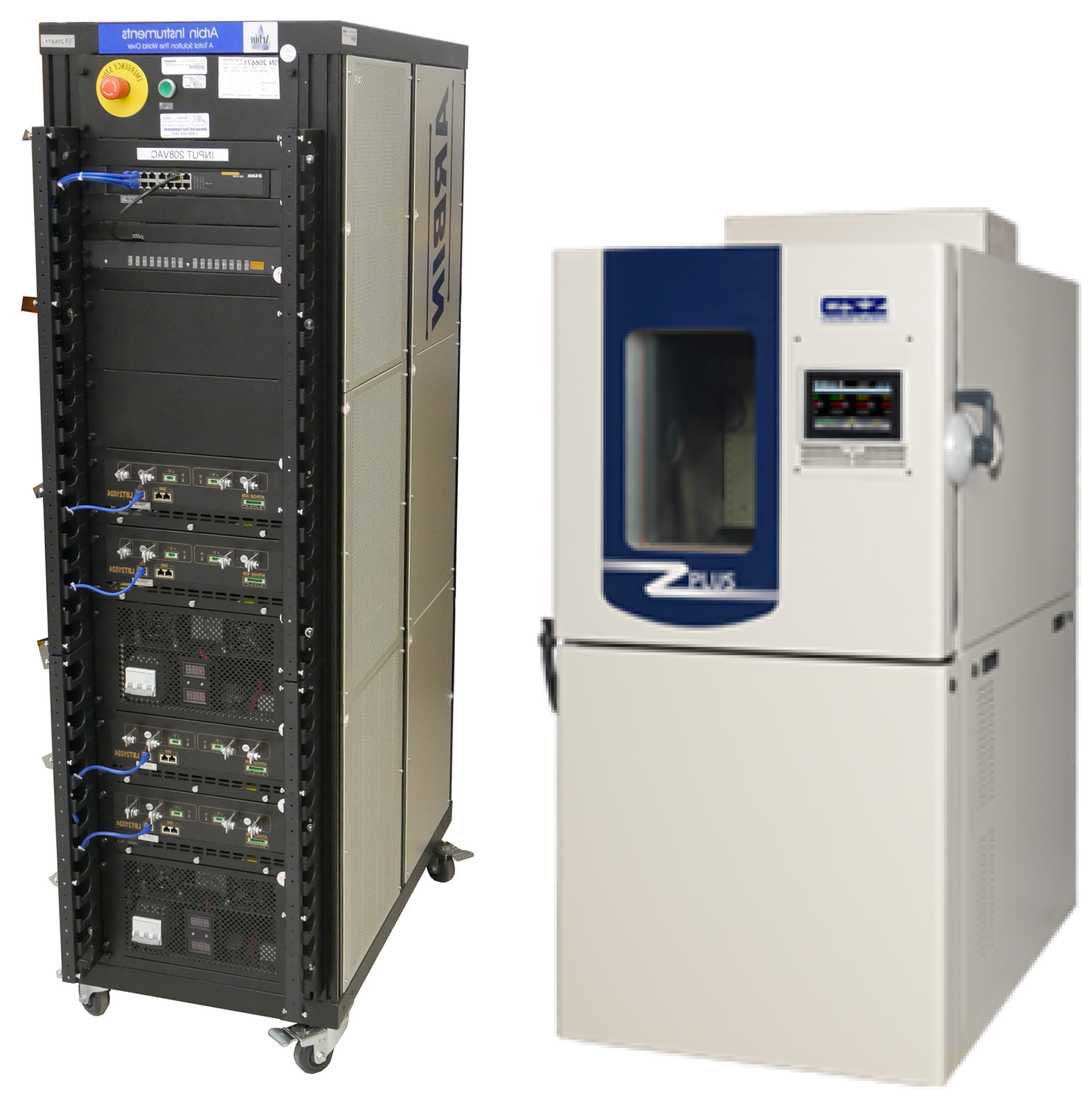Figure 1a shows an 8-channel battery cell cycler made by Arbin; this device allows the collection of battery characterization data simultaneously from eight battery cells at the same time. Moreover, the battery needs to be kept at a fixed temperature in an environmental chamber during the OCV–SOC characterization. Figure 1b shows an environmental chamber made by Cincinnati Subzero for battery research.

Figure 1. Scientific-grade equipment used to collect OCV characterization data.

The data collection for the OCV characterization is designed in a way that the effects of the hysteresis and relaxation phenomenons of the battery can be nullified in the obtained OCV model. Depending on the OCV modeling approach, the data collection may also vary. In [5], a slow-rate data collection approach is demonstrated on various existing OCV–SOC models for parameter estimation. In this approach, a fully charged battery is very slowly discharged (typically at a C/30 rate) using a constant current until it becomes empty. Then, it is charged back to full charge using the same amount of constant current. This entire discharge–charge process takes 60 h. Constant current ensures that the capacitances of the equivalent circuit model remain saturated; a very low magnitude of current assures that the hysteresis effect can be approximated as an equivalent resistance. By measuring the voltage and current values during this entire discharge/charge process, the OCV–SOC parameters are obtained. It is preferred that these data are free of measurement noise and bias. High-precision battery cyclers can maintain constant currents with very little variation and can measure and store voltage and current with very little measurement noise.

Different OCV–SOC models exist in the literature to adequately represent the OCV curve in the entire span of SOC (0–100%). Several reasons can be stated as to why many variations in the parametric expression for different models exist. Each model approximates the OCV curve differently for the lower (≈0–30%) and higher (≈80–100%) ranges of SOC. For example, the OCV–SOC relationship is quite approximately a straight line between 30% and 80% of the SOC. The straight-line model is the most simplistic approach to OCV–SOC characterization, needing just two parameters; however, the accuracy of the model is compromised at very low and very high SOC regions. In order to improve the accuracy of representation, higher-order empirical models utilizing special functions, such as the polynomial [6], trigonometric [7], logarithmic [8,9,10,11], and exponential functions [12,13], are used. The estimated parameters using these special functions often need to be represented up to their nth decimal digit for the precise estimation of SOC (for example, in combined+3 model [11], n needs to be as high as six to preserve the modeling accuracy). This directly translates to using a large number of bits to completely represent, store, and process these parameters. 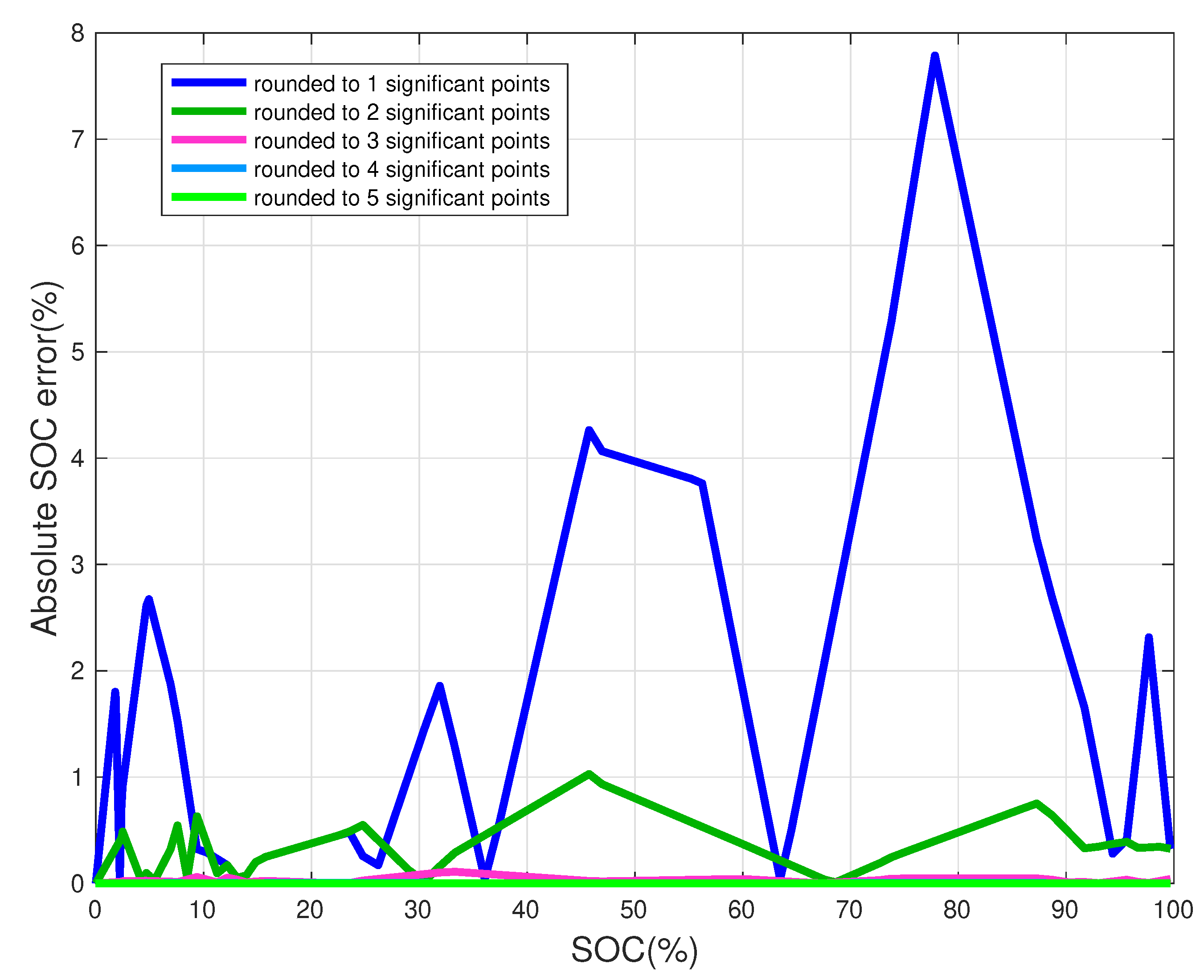However, many practical applications (see examples form Texas Instruments [14] and Maxim Integrated [15]) only allow low-bit processing for BFGs, requiring the traditional OCV–SOC parameters to be rounded. Rounding has been shown to significantly alter the model representation, resulting in poor SOC estimation accuracy [16]. To be able to represent the OCV–SOC curve in low-computing environments precisely, tabular models can be used [16]. Finally, variations in battery chemistries are also a driving factor for varied OCV–SOC representations.

Different OCV–SOC models vary in their formulation, in the methods of estimation of their parameters, and eventually in the resulting SOC estimation error. While accurate SOC estimation is crucial, selecting a model solely based on the accuracy of estimation may not be suitable in many applications. For example, in high-power restrictive medical equipment, such as an implantable cardiac pacemaker, reducing computational complexity is crucial [17], while the accuracy of SOC estimation is also important. In the case of electric vehicles (EV), for example, drivers are found to experience range anxiety [18]. Here, the accuracy of SOC estimation is crucial, and the computational requirement for SOC estimation is not a concern. These examples illustrate that BMS designers need to take multiple constraints before selecting an OCV–SOC model. There needs to be a systematic approach to selecting a particular OCV–SOC model from the numerous models presented in the literature for a specific application.

This paper presents a systematic approach to OCV–SOC model selection based on multiple selection criteria. First, each model is individually evaluated in terms of the different metrics considered—accuracy, numerical stability, computational complexity, and system requirements. The computed metrics for each model are then ranked in increasing order based on the definition of the metric. For example, the model with the highest accuracy is ranked first under the “accuracy” category. However, for computational complexity, the model with the lowest computational complexity is ranked first. Once the individual metrics are ranked, an overall ranking system, based on the Borda count voting system [19], is pursued to combine all the metrics. The Borda count voting system ranks the candidate models in the order of the most preferred to the least based on all the selection criteria. The objective of this work is to give the reader a systematic procedure for selecting a model based on different criteria, depending on the application of their choice. Finally, the proposed approach is demonstrated using the OCV–SOC characterization data collected from a cylindrical battery cell.

In Section 2, the eligibility criteria for the literature review and the summary of OCV–SOC characterization is provided. Section 3 lists possible OCV models that have been used in the literature for OCV characterization. These models are classified under four categories: linear models, nonlinear models, hybrid models, and tabular models. Section 4 details approaches to estimate the parameters for the four types of models presented in Section 3. Given all the possibilities for OCV modeling, which model is suitable for a particular BMS design? Section 5 answers this question by introducing several model selecting metrics. Finally, Section 6 provides an example of selecting a model under multiple constraints.

2. Literature Review

The initial search involved the keyword ‘OCV model-based SOC estimation’, which returned 41 articles on engineering village [20]. Among them, the articles meeting the following inclusion criteria were chosen: (i) written in English, (ii) published in peer-reviewed journals, and (iii) empirical, tabular, and/or fused models. In total, 26 articles were selected based on the inclusion criteria. In addition, a few other articles were also selected from the authors’ previous work on OCV–SOC characterization [5].

A summary of the existing OCV modeling approaches from the articles is provided in Table 1. All the models listed in Table 1 vary in their formulation, in the methods of estimation of such parameters, and eventually in the errors of estimation of SOC. In Section 3, select empirical OCV–SOC modeling approaches from Table 1 are grouped into four categories: linear, nonlinear, hybrid, and tabular. The mathematical equations and parameterization of these approaches are also described in the next section.

Table 1. Literature review OCV modeling approaches.

Ref.	Description	Category
[12,21,22]	A double exponential model with a quadratic term with five parameters each to represent the charging and discharging curves is proposed. It is shown that the proposed model is the most precise among the models compared in terms of evaluation of the root mean square error (RMSE) and $R^2$ metrics.	nonlinear
[23]	In addition to the polynomial terms, a fractional-order model is proposed to show OCV as a fractional-order function of SOC.	Linear
[6,24]	A third-order polynomial combined with exponential terms with six parameters is proposed to denote OCV as a function of SOC.	nonlinear
[8,9,25,26]	A hybrid empirical battery model combining Shepherd, Unnewehr universal, and Nernst models is used to represent the OCV curve.	Linear
[27]	OCV is modeled as the sum of logarithmic, linear, and shifted exponential functions of the SOC with six parameters.	nonlinear
[28,29]	An eighth-order polynomial model with nine parameters is used to demonstrate the OCV–SOC relationship.	Linear
[30]	A complex OCV model with twelve parameters, comprised of linear and shifted exponential terms is proposed.	nonlinear
[31]	A fused OCV model is proposed, where the OCV curve is segmented to local sub-intervals and then fused together. Appropriate models are used to fit the curve in the local regions. The OCV sub-models are then fused into a fusional OCV model. A fourth-degree polynomial and logarithmic and exponential functions are used in each of the local sub-regions.	Hybrid nonlinear
[32]	In addition to the dependence of OCV on SOC, cell voltage recovery and hysteresis are factored in the modeling of the OCV–SOC curve, increasing the total number of parameters to be estimated.	nonlinear
[33,34,35]	An OCV–SOC lookup table is built from the low-current OCV experimental data by linear interpolation of the battery voltages at two consecutive charge and discharge cycles.	Tabular
[36]	An approach based on piecewise cubic Hermite interpolation is used to build the OCV model.	Hybrid
[37]	An improved combined model for modeling the OCV–SOC relationship.	Linear
[13,24,38,39]	Exponential modeling with variations in OCV–SOC formulations.	nonlinear
[7]	Electrical model to determine the short-term battery behavior	nonlinear

3. Empirical OCV–SOC Models

The open-circuit voltage of the battery has a monotonically increasing relationship to the SOC. This relationship is the backbone of the state-of-charge estimation algorithms, i.e., by measuring the voltage across the battery terminals, its SOC can be estimated as long as the OCV–SOC parameter is already available.

3.1. Linear Regression Models

A linear OCV model can be written as

$$\begin{array}{c}\hfill \begin{array}{c}\hfill V_{\circ }\left(s\right)=\sum _{i=0}^{L-1}{p}_i\left(s\right)k_i=\mathbf{p}{\left(s\right)}^T\mathbf{k}\end{array}\end{array}$$

(1)

where $V_{\circ }\left(s\right)$ denotes the OCV, $s\in [0,1]$ denotes the SOC, and p${\left(s\right)}^T=[p_0\left(s\right),p_1\left(s\right),\dots ,p_{L-1}\left(s\right)]$ is a row vector of linear/nonlinear functions of s, and k $= {[k_0,k_1,\dots ,k_{L-1}]}^T$ is the OCV parameter vector. The simplest form of the linear OCV model is the Unnewehr universal model [26,40] which is simply a straight line:

$$\begin{array}{c}\hfill \begin{array}{c}\hfill V_{\circ }\left(s\right)={\mathbf{p}\left(s\right)}^T\mathbf{k}=k_0+k_{1}s\end{array}\end{array}$$

(2)

which has p${\left(s\right)}^T=\left[1s\right]$ and k $= {\left[k_0{k}_1\right]}^T$. Some linear models introduced in the literature are listed below:

• Shepherd model [26,41]

  $$\begin{array}{c}\hfill V_{\circ }\left(s\right)=k_0+\frac{k_1}{s}\end{array}$$

  (3)
• Nernst model [8,9,26]

  $$\begin{array}{c}\hfill V_{\circ }\left(s\right)=k_0+k_{1}ln\left(s\right)+k_{2}ln(1-s)\end{array}$$

  (4)
• Combined model [10]

  $$\begin{array}{c}\hfill V_{\circ }\left(s\right)=k_0+\frac{k_1}{s}+k_{2}s+k_{3}ln\left(s\right)k_{4}ln(1-s)\end{array}$$

  (5)
• Combined+3 model [11]

  $$\begin{array}{cc}\hfill V_{\circ }\left(s\right)=& \hfill k_0+\frac{k_1}{s}+\frac{k_2}{s^2}+\frac{k_3}{s^3}+\frac{k_4}{s^4}+k_{6}s+k_{6}ln\left(s\right)+k_{7}ln(1-s)\hfill \end{array}$$

  (6)
• Polynomial model [6]

  $$\begin{array}{cc}\hfill V_{\circ }\left(s\right)=& \hfill k_0+k_{1}s+\dots +k_m{s}^m+k_{m+1}{s}^{-1}+\dots +k_{m+n}{s}^{-n}\hfill \end{array}$$

  (7)
• Exponential model [27]

  $$\begin{array}{cc}\hfill V_{\circ }\left(s\right)=& \hfill k_0+k_1{e}^s+\dots +k_m{e}^{s^m}+k_{m+1}{e}^{-s}+\dots +k_{m+n}{e}^{-s^n}\hfill \end{array}$$

  (8)

The parameters of all the linear models from (2) to (8) can be estimated through the linear least square estimation approach. Section 4 demonstrates an example of linear least squares model parameter estimation in detail.

3.2. Nonlinear Regression Models

The nonlinear model is written in general form as

$$\begin{array}{c}\hfill V_{\circ }\left(s\right)=f(s,\mathbf{k})\end{array}$$

(9)

where k denotes a vector of model parameters. Similar to before, the number of parameters, i.e., the length of k, depends on the model. Some possible nonlinear models from the literature are listed below:

• Double exponential model [12].

  $$\begin{array}{c}\hfill V_{\circ }\left(s\right)=k_0+k_{1}s+k_2\left(1-e^{-k_{3}s}\right)+k_4\left(1-e^{-\frac{k_5}{1-s}}\right)\end{array}$$

  (10)
• Nonlinear exponential model-1 [13]

  $$\begin{array}{c}\hfill V_{\circ }\left(s\right)=k_0-\frac{k_1}{s}+k_2{e}^{-k_3(1-s)}\end{array}$$

  (11)
• Nonlinear exponential model-2 [24]

  $$\begin{array}{c}\hfill V_{\circ }\left(s\right)=k_0{e}^{-k_{1}s}+k_2+k_{3}s+k_4{s}^2+k_5{s}^3\end{array}$$

  (12)
• Nonlinear exponential model-3 [38,39]

  $$\begin{array}{c}\hfill V_{\circ }\left(s\right)=a_1{e}^{\left(b_{1}s\right)}+a_2{e}^{\left(b_{2}s\right)}+c{s}^2\end{array}$$

  (13)
• Rational approximant [42]

  $$\begin{array}{c}\hfill V_{\circ }\left(s\right)=\frac{{\displaystyle \sum _{i=0}^m}{k}_i{s}^i}{1+{\displaystyle \sum _{j=1}^n}{k}_{j+m}{s}^j},m\ge 0,n>0\end{array}$$

  (14)
• Sum of sine model [7]

  $$\begin{array}{c}\hfill V_{\circ }\left(s\right)=a_1\sin (b_{1}s+c_1)+a_2\sin (b_{2}s+c_2)+a_3\sin (b_{3}s+c_3)\end{array}$$

  (15)

3.3. Hybrid or Piecewise Linear Models

Hybrid modeling seeks to approximate the OCV–SOC curve as piecewise linear functions. One section of the OCV curve, where SOC $\in \left[0\zeta \right]$, is modeled using one of the linear functions presented in Section 3.1, and the other section of the OCV curve, where SOC $\in \left[\zeta 1\right]$, is modeled using another the linear function of Section 3.1. The advantage of hybrid modeling is that it offers better accuracy and computational efficiency in favor of more complex models. The formal representation of the two-piecewise linear OCV model is as follows:

$$\begin{array}{c}\hfill V_{\circ }\left(s\right)=\left\{\begin{array}{cc}\hfill {{\mathbf{p}}_i\left(s\right)}^T{\mathbf{k}}_i\hfill & \hfill \mathrm{if} s\ge \zeta \hfill \\ \hfill {{\mathbf{p}}_j\left(s\right)}^T{\mathbf{k}}_j\hfill & \hfill \mathrm{if} s<\zeta \hfill \end{array}\right.\end{array}$$

(16)

where each of ${\mathbf{p}}_i\left(s\right)$ and ${\mathbf{p}}_j\left(s\right)$ denote one of the several linear OCV models in Section 3.1. When ${\mathbf{p}}_i\left(s\right)$ and ${\mathbf{p}}_j\left(s\right)$ represent two straight lines, the minimum number of parameters will be five: two parameters each for the straight lines and $\zeta$. These five parameters can be obtained using the hybrid optimization step briefed in Section 4.

3.4. Tabular Model

The OCV–SOC characterization approaches discussed so far required the estimation of a parameter vector k. Depending on the model, the parameter k may require a high-precision floating point system for storage in a BMS. The tabular model stores the OCV–SOC pairs as a table. Table 2 shows an 11-point OCV–SOC table. The advantage of storing the OCV–SOC characterization as a table is that it does not require a high-precision floating point system to store the values. The accuracy of the OCV–SOC table is not likely to be severely compromised by rounding these values (based on the available memory system). Some battery fuel gauging (BFG) algorithms require the derivative of the OCV function to recursively estimate SOC using filtering techniques. Hence, it is desired for an OCV–SOC table to store the derivatives as well.

Table 2. A Sample OCV–SOC table.

s	${\mathit{V}}_{\circ }\left(\mathit{s}\right)$	$\frac{{\mathit{dV}}_{\circ }\left(\mathit{s}\right)}{\mathit{ds}}$
0.0	3.0519	44.4073
0.1	3.6594	0.6830
0.2	3.7167	0.8131
0.3	3.7611	0.4807
0.4	3.7915	0.4393
0.5	3.8275	0.6055
0.6	3.8772	0.8113
0.7	3.9401	0.9777
0.8	4.0128	1.0915
0.9	4.0923	1.1822
1.0	4.1797	1.3405

Table 2 was formed by uniformly sampling SOC. The approximation error can be shown to be proportional to the curvature of the OCV–SOC curve. This implies a better strategy is needed to sample the OCV–SOC values for storage as a table. Section 4.4 details an improved approach to obtain samples for OCV–SOC tables.

4. OCV–SOC Model Parameter Estimation

In this section, the detailed approach to estimating the OCV–SOC parameters, from data collection to parameter estimation, is presented. The data collection needs to be performed using professional, high-precision battery cyclers that have very low measurement noise. Figure 1a shows an Arbin battery cycler that can be programmed to execute the above data collection procedure. It is also important to keep the temperature fixed, because the change in temperature translates to changes in internal resistance. A professional environmental chamber, similar to the one shown in Figure 1b, needs to be used to keep the temperature fixed during the experiment.

The data for OCV characterization needs to be collected in a specific way such that the parameter estimation will not be affected by the elements of the equivalent circuit model in a battery.

The following procedure needs to be followed for the data collection of OCV–SOC characterization:

• Fully charge the battery at room temperature. In order to fully charge the battery, the constant-current (CC) constant-voltage (CV) approach can be used. The CV charging is terminated when the charging current i falls below $i_c<C/N$.
• Bring the battery to a fixed temperature in which the OCV characterization is to be performed.
• Slow-discharge the battery with a discharging current of $i_d=C/N$ rate until the terminal voltage reaches $v={\mathrm{OCV}}_{\min }$. Let us denote the total discharge time as $T_d.$
• Slow-charge the battery with a charging current of $i_c=C/N$ rate until the terminal voltage reaches $v={\mathrm{OCV}}_{\max }.$ Let us denote the total discharge time as $T_c.$

Here, the term $C/N$ is used to indicate the magnitude of the current. For example, let us say the manufacturer rated capacity of the battery is $C=1.5\mathrm{Ah}.$ Then, the current at $C/30$ rate is $i_{\mathbf{c}}=i_{\mathrm{d}}=1.5/30=0.05\mathrm{A}.$

The voltage and current data in the discharge and charge process is logged at a reasonable sampling rate. Considering that the discharge rate is very low, a sampling time of $\Delta =60$ seconds is sufficient for OCV modeling. When N is set to $N=30,$ i.e., when the discharging and charging currents are set to $i_{\mathrm{c}}=i_{\mathrm{d}}=C/30,$ the number of samples collected during discharging is $k_d=30\times 60=1800.$ It must be noted that the actual number of $k_d$ may vary depending on the available capacity of the battery, regardless of the labeled capacity.

Using the notations discussed so far, let us denote the voltage and current data collected during the discharging step (step 3) as $v\left(1\right),v\left(2\right),\dots ,v\left(k_d\right)$ and $i\left(1\right),i\left(2\right),\dots ,i\left(k_d\right)$, respectively. Similarly, let us denote the voltage and current data collected during the charging step (step 4) as $v(k_d+1),v(k_d+2),\dots ,v\left(k_c\right)$ and $i(k_d+1),i(k_d+2),\dots ,i\left(k_c\right)$, respectively. Using the notations introduced so far, the discharging and charging time can be written as

$$\begin{array}{cc}\hfill T_d& \hfill =\Delta k_d\hfill \end{array}$$

(17)

$$\begin{array}{cc}\hfill T_c& \hfill =\Delta (k_c-k_d)\hfill \end{array}$$

(18)

The charge/discharge capacities of the battery are defined as

$$\begin{array}{cc}\hfill Q_c& \hfill =i_c{T}_c\hfill \end{array}$$

(19)

$$\begin{array}{cc}\hfill Q_{\mathrm{d}}& \hfill =i_{\mathrm{d}}{T}_d\hfill \end{array}$$

(20)

where Q_c and Q_d denote the charge and discharge capacities, respectively.

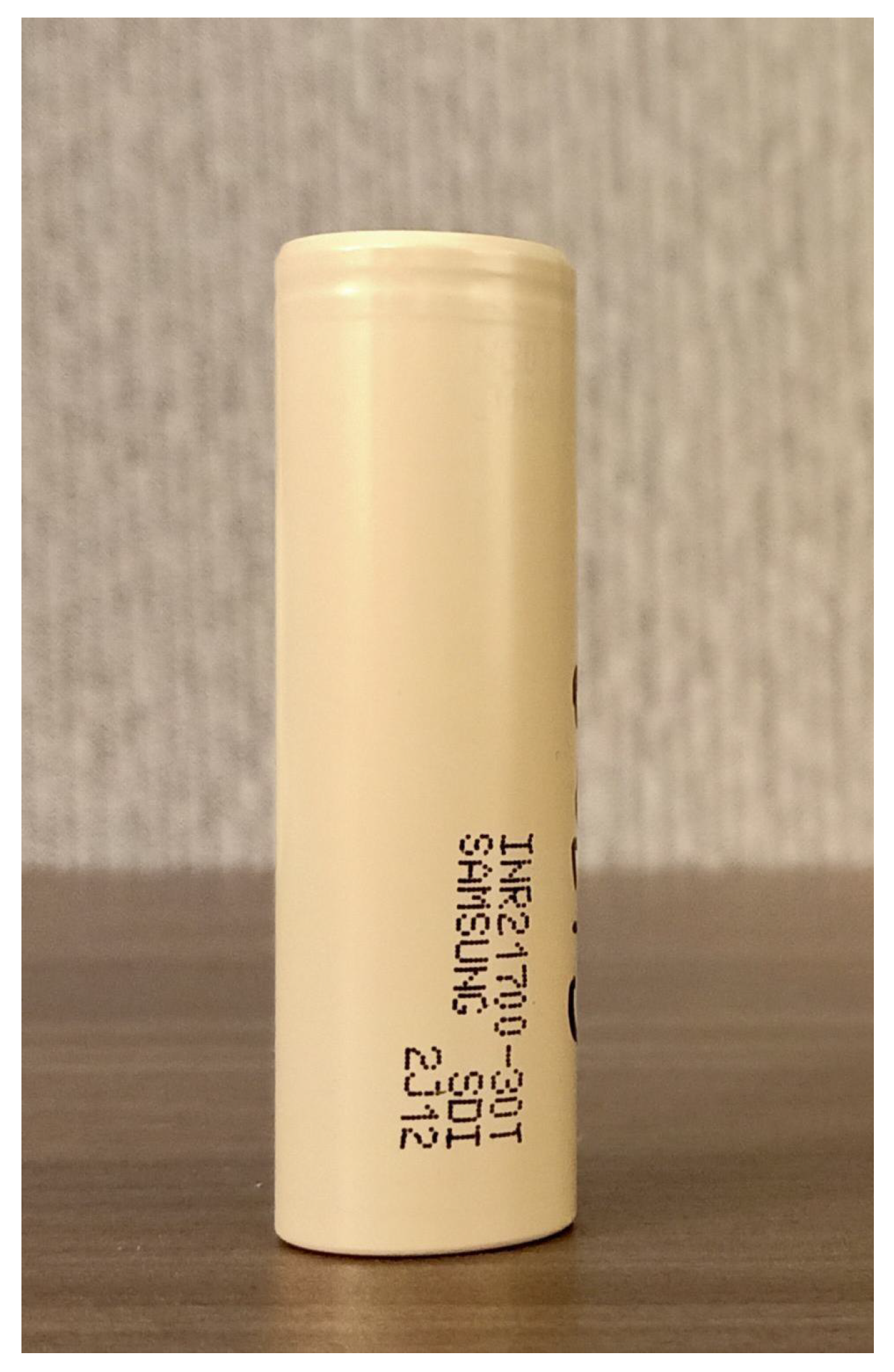
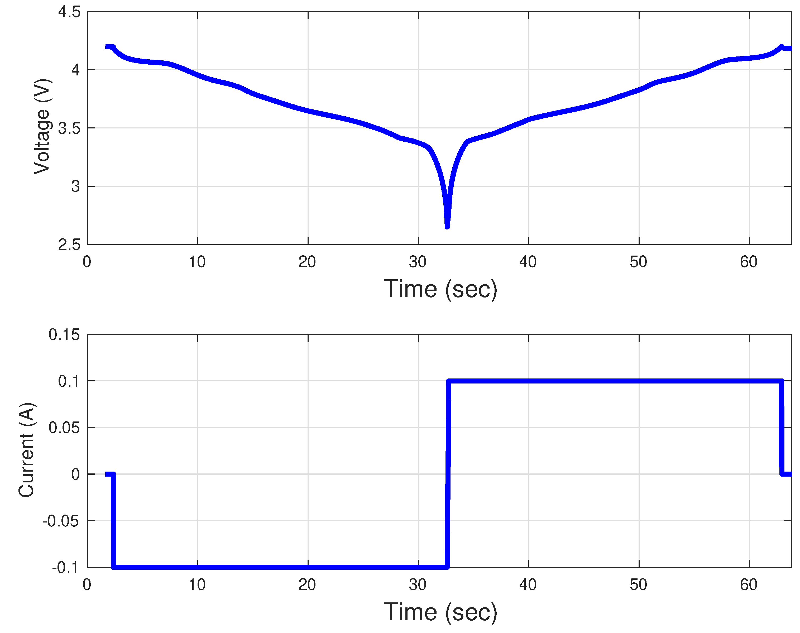
The data for the demonstration was generated using the Samsung-30T INR21700 battery, shown in Figure 2. The features of the battery are summarized in Table 3. Figure 3 shows the voltage $v\left(k\right)$ and current $i\left(k\right)$ measurements during the discharging and charging steps of the data collection [43]. The remainder of this section details how these data are used to estimate the OCV parameters of a battery.

Figure 2. Samsung-30T INR21700 Li-ion battery.

Table 3. Specifications of Li-ion battery.

Specification	Unit
Nominal capacity	3000 mAh
Maximum continuous discharge current	35 A
Nominal voltage	3.6 V
Height	70 mm
Diameter	21 mm
Weight	70 g
Internal resistance	15 m$\Omega$

Figure 3. Measured voltage and current during charge and discharge at 25 °C [43].

First, let us define the SOC at a given time as

$$\begin{array}{c}\hfill s\left(k\right)\triangleq s\mathrm{at} \mathrm{time} k\end{array}$$

(21)

where the notation ≜, that reads “defined as”, is used to assign a new variable name with a slightly different context, e.g., the value s at time k is defined as $s\left(k\right)$ in (21). The true SOC at time k can be recursively computed using the Coulomb counting equation:

$$\begin{array}{c}\hfill s(k+1)=s\left(k\right)+\frac{{\Delta }_{k}i\left(k\right)}{3600Q}\end{array}$$

(22)

where ${\Delta }_k=\Delta$ is the time difference between two measurements in seconds, $i\left(k\right)$ is the current (in Amperes) through the battery, and

$$\begin{array}{c}\hfill Q=\left\{\begin{array}{cc}{Q}_d& i\left(k\right)\le 0\\ Q_c& i\left(k\right)>0\end{array}\right.\end{array}$$

(23)

is the battery capacity in Ampere hour (Ah).

Remark 1.

It is important to note that although Coulomb counting is the easiest approach to calculate SOC at any given instant, it suffers from (i) initial SOC error, (ii) current measurement errors, (iii) current integration error, (iv) timing oscillator error, and (v) uncertainty in battery capacity [44].

So far, $v\left(k\right)$ and $i\left(k\right)$ denoted the voltage across the battery terminals and current through the battery, respectively, during the experiment. Even in high-precision systems, the measured quantities will incur some measurement noise. Let us denote the measured voltage and current using the following

$$\begin{array}{cc}\hfill z_v\left(k\right)=& \hfill v\left(k\right)+n_v\left(k\right)\hfill \end{array}$$

(24)

$$\begin{array}{cc}\hfill z_i\left(k\right)=& \hfill i\left(k\right)+n_i\left(k\right)\hfill \end{array}$$

(25)

where $v\left(k\right)$ and $i\left(k\right)$ denote the true voltage across the battery terminals and current through the battery, $n_v\left(k\right)$ denotes the voltage measurement noise that is assumed to be zero-mean white with standard deviation (s.d.) ${\sigma }_v$, and $n_i\left(k\right)$ denotes the current measurement noise that is assumed to be zero-mean white with s.d. ${\sigma }_i$.

During the OCV experiment, i.e., when the battery is being slowly charged or discharged, the terminal voltage can be written as

$$\begin{array}{c}\hfill z_v\left(k\right)=V_{\circ }\left(s\left(k\right)\right)+h\left(k\right)+i\left(k\right)R_{\mathrm{int}}+n_v\left(k\right)\end{array}$$

(26)

where $h\left(k\right)$ is the hysteresis voltage. By substituting $i\left(k\right)=z_i\left(k\right)-n_i\left(k\right)$ in (26), it can be rewritten in terms of the measured current as follows

$$\begin{array}{c}\hfill z_v\left(k\right)=V_{\circ }\left(s\left(k\right)\right)+h\left(k\right)+z_i\left(k\right)R_{\mathrm{int}}+n\left(k\right)\end{array}$$

(27)

where the noise term $n\left(k\right)$ can be shown to be zero-mean with ${\sigma }_z={\sigma }_v^2+{\sigma }_i^2{R}_{\mathrm{int}}^2$ as the s.d.

Since the OCV test is performed at a very low current, it can be assumed that the hysteresis is proportional to the current only, i.e.,

$$\begin{array}{c}\hfill h\left(k\right)\propto i\left(k\right)\end{array}$$

(28)

Hence, (27) can be rewritten as

$$\begin{array}{c}\hfill z_v\left(k\right)=V_{\circ }\left(s\left(k\right)\right)+z_i\left(k\right)R_{\mathrm{eff}}+n\left(k\right)\end{array}$$

(29)

where the effective resistance

$$R_{\mathrm{eff}}=R_{\mathrm{int}}+R_{\mathrm{h}}$$

(30)

is the summation of the internal resistance $R_{\mathrm{int}}$ and the hysteresis equivalent resistance $R_{\mathrm{h}}.$

The goal is to estimate the parameters that define the OCV $V_{\circ }\left(s\left(k\right)\right)$ in (29). Depending on how the OCV is defined in Section 3, the parameter estimation approach needs to be different. For linear models summarized in Section 3.1, the linear least squares method is explained in Section 4.1. For nonlinear models summarized in Section 3.2, the linear least squares method is explained in Section 4.2. Parameter estimation of the hybrid linear models of Section 3.3 is summarized in Section 4.3, and Section 4.4 summarizes approaches to create OCV–SOC tables.

4.1. Linear Least Squares

The linear OCV–SOC model parameter estimation approach is described in this section using one of the linear models, the combined+3 model (6), presented in Section 3.1. A similar approach can be followed to estimate all other linear models.

Using vector notations, the observation model in (29) can be written as,

$$\begin{array}{cc}\hfill z_v\left(k\right)& \hfill =\underset{{\mathbf{p}\left(k\right)}^T}{\underbrace{\left[{\mathbf{p}}_{\circ }{\left(s\left(k\right)\right)}^{T}i\left(k\right)\right]}}\underset{\mathbf{k}}{\underbrace{\left[\begin{array}{c}{\mathbf{k}}_{\circ }\\ R_{\mathrm{eff}}\end{array}\right]}}+n_v\left(k\right)\hfill \end{array}$$

(31)

where

$$\begin{array}{c}\hfill {\mathbf{k}}_{\circ }={\left[k_0{k}_1{k}_2{k}_3{k}_4{k}_5{k}_6{k}_7\right]}^T\end{array}$$

(32)

and

$$\begin{array}{cc}\hfill {\mathbf{p}}_{\circ }{\left(s\left(k\right)\right)}^T=[& \hfill 1\frac{1}{s\left(k\right)}\frac{1}{s^2\left(k\right)}\frac{1}{s^3\left(k\right)}\frac{1}{s^4\left(k\right)}s\left(k\right)ln\left(s\left(k\right)\right)ln(1-s\left(k\right))]\hfill \end{array}$$

(33)

By considering a batch of N voltage observations, (31) can be written as

$$\begin{array}{cc}& \hfill \mathbf{v} =\mathbf{P}\mathbf{k} + \mathbf{n}\hfill \end{array}$$

(34)

where

$$\begin{array}{cc}& \hfill \mathbf{v}={\left[z_v\left[1\right]z_v\left[2\right]\dots z_v\left[k_d\right]\right]}^T\hfill \end{array}$$

(35)

$$\begin{array}{cc}& \hfill \mathbf{P}={\left[\mathbf{p}\left[1\right]\mathbf{p}\left[2\right]\dots \mathbf{p}\left[k_d\right]\right]}^T\hfill \end{array}$$

(36)

$$\begin{array}{cc}& \hfill \mathbf{n}={\left[n\left[1\right]n\left[2\right]\dots n\left[k_d\right]\right]}^T\hfill \end{array}$$

(37)

$$\begin{array}{cc}& \hfill \mathbf{k}={\left[k_0{k}_1{k}_2{k}_3{k}_4{k}_5{k}_6{k}_7{R}_{\mathrm{eff}}\right]}^T\hfill \end{array}$$

(38)

The least squares estimate of the parameter vector is given by

$$\begin{array}{c}\hfill \widehat{\mathbf{k}}={\left({\mathbf{P}}^T\mathbf{P}\right)}^{-1}{\mathbf{P}}^T\mathbf{v}\end{array}$$

(39)

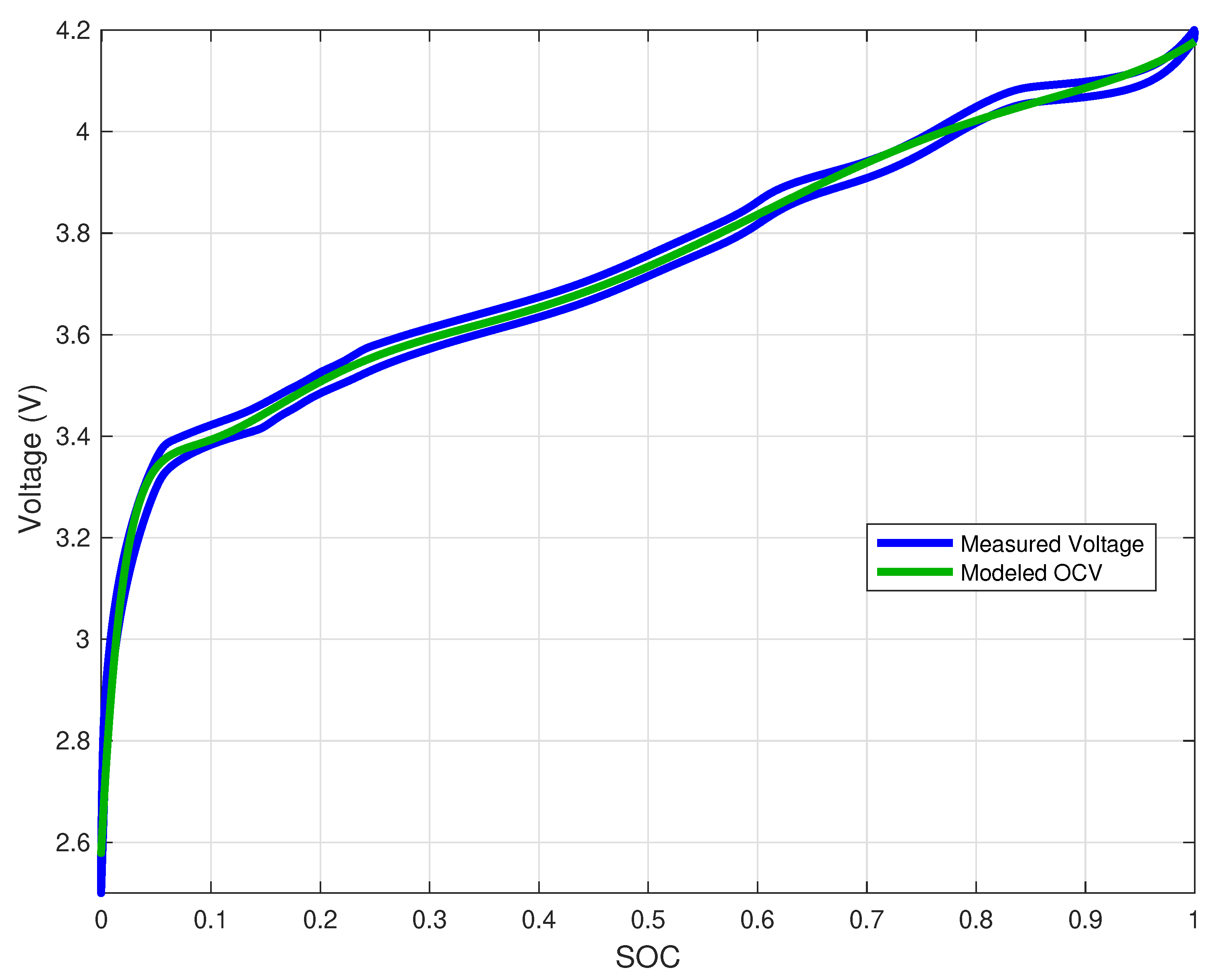
Now, for a given SOC, the corresponding OCV estimate ${\widehat{V}}_{\circ }\left(s\right)$ is computed as

$$\begin{array}{c}\hfill {\widehat{V}}_{\circ }\left(s\right)={\mathbf{p}}_{\circ }{\left(s\right)}^T{\widehat{\mathbf{k}}}_{\circ }\end{array}$$

(40)

where ${\widehat{\mathbf{k}}}_{\circ }$ is formed by the first 8 elements of $\widehat{\mathbf{k}}$. Given the voltage and current data, $v\left(1\right),v\left(2\right),\dots ,v\left(k_c\right)$ and $i\left(1\right),i\left(2\right),\dots ,i\left(k_c\right)$, respectively, corresponding to the plot in Figure 3, the following Matlab codes will generate the parameter vector t corresponding to the combined+3 model and generate Figure 4.

Figure 4. OCV model of a Li-ion battery.

The estimated OCV parameters are

$$\begin{array}{c}\hfill k_0=-6.6266,k_1=157.3029,k_2=-26.8590,\end{array}$$

(41)

$$\begin{array}{c}\hfill k_3=2.9721,k_4=-0.1440,k_5=-127.7601,\end{array}$$

(42)

$$\begin{array}{c}\hfill k_6=224.5953,k_7=-1.8463,k_8=0.1984\end{array}$$

(43)

and the estimated effective resistance is $R_{\mathrm{eff}}=0.14809\Omega .$

4.2. Nonlinear Least Squares

For nonlinear models, we rewrite (34) in the following form

$$\begin{array}{cc}& \hfill \mathbf{v}={\mathbf{v}}_{\circ }\left({\mathbf{k}}_{\circ }\right)+\mathbf{i}{R}_{\mathrm{eff}}+\mathbf{w}\hfill \end{array}$$

(44)

where

$$\begin{array}{c}\hfill \begin{array}{cc}& \mathbf{k}={\left[{\mathbf{k}}_{\circ }{R}_{\mathrm{eff}}\right]}^T\hfill \\ \hfill {\mathbf{v}}_{\circ }\left({\mathbf{k}}_{\circ }\right)& \hfill ={\left[V_{\circ }(s\left(1\right),{\mathbf{k}}_{\circ })\dots V_{\circ }(s\left(k_c\right),{\mathbf{k}}_{\circ })\right]}^T\hfill \\ & \mathbf{i}=\left[i\left(1\right)i\left(2\right)\dots ,i\left(k_c\right)\right]\hfill \end{array}\end{array}$$

(45)

and w is the noise vector.

The coefficients of the nonlinear regression-based models were computed using the Matlab optimization toolbox function for nonlinear least squares lsqnonlin. The nonlinear least squares problem solves the following problem

$$\begin{array}{cc}\hfill \widehat{\mathbf{k}}& \hfill =arg\underset{\mathbf{k}}{min}\parallel \mathbf{v}-\widehat{\mathbf{v}}\parallel \hfill \end{array}$$

(46)

4.3. Hybrid Estimation

Hybrid model parameters are estimated using constrained least squares estimation techniques. The following constraints are used:

• The derivative is always positive. This constraint ensures that the OCV is a monotonically increasing function in terms of SOC.
• Both piecewise functions and their first and second derivatives are the same at the transition point $\zeta .$ This constraint ensures that the transition between one piecewise linear function to another is seamless and without any sudden changes in characteristics.

Let us rewrite the linear observation model (34) as

$$\begin{array}{c}\hfill \begin{array}{cc}\hfill {\mathbf{v}}_1& \hfill ={\mathbf{P}}^1\left(s\right){\mathbf{k}}_1+{\mathbf{n}}_{1}s\in [0,\zeta ]\hfill \\ \hfill {\mathbf{v}}_2& \hfill ={\mathbf{P}}^2\left(s\right){\mathbf{k}}_2+{\mathbf{n}}_{2}s\in [0,\zeta ]\hfill \end{array}\end{array}$$

(47)

The observation model (47) can be combined as follows

$$\begin{array}{cc}\hfill \tilde{\mathbf{v}}& \hfill =\left[\begin{array}{c}{\mathbf{v}}_1\\ {\mathbf{v}}_2\end{array}\right]=\left[\begin{array}{cc}{\mathbf{P}}^1\left(s\right)& \underset{\_}{0}\\ \underset{\_}{0}& {\mathbf{P}}^2\left(s\right)\end{array}\right]\left[\begin{array}{c}{\mathbf{k}}_1\\ {\mathbf{k}}_2\end{array}\right]+\left[\begin{array}{c}{\mathbf{n}}_1\\ {\mathbf{n}}_2\end{array}\right]\hfill \\ \hfill \tilde{\mathbf{v}}& =\tilde{\mathbf{P}}\left(s\right)\tilde{\mathbf{k}}+\tilde{\mathbf{n}}\hfill \end{array}$$

(48)

The model parameters of a hybrid, bi-linear OCV–SOC function are obtained through the following optimization:

$$\begin{array}{cc}\hfill \{{\widehat{\mathbf{k}}}_1,{\widehat{\mathbf{k}}}_2\}& \hfill =arg\underset{{\widehat{\mathbf{k}}}_1,{\widehat{\mathbf{k}}}_2}{min}∥\left(\tilde{\mathbf{P}}\left(s\right)\tilde{\mathbf{k}}-\tilde{\mathbf{v}}\right)∥\hfill \end{array}$$

(49)

subject to

$$\begin{array}{c}\hfill \begin{array}{cc}\hfill \frac{d{\mathbf{P}}^i{\widehat{\mathbf{k}}}_1}{ds}& \hfill >0\hfill \\ \hfill \frac{d{\mathbf{P}}^j{\widehat{\mathbf{k}}}_2}{ds}& \hfill >0\hfill \\ \hfill {\left.{\mathbf{P}}^i\left(s\right){\widehat{\mathbf{k}}}_1\right|}_{s=\zeta }-{\left.{\mathbf{P}}^j\left(s\right){\widehat{\mathbf{k}}}_2\right|}_{s=\zeta }& \hfill =0\hfill \\ \hfill {\left.\frac{d{\mathbf{P}}^i\left(s\right){\widehat{\mathbf{k}}}_1}{ds}\right|}_{s=\zeta }-{\left.\frac{d{\mathbf{P}}^j\left(s\right){\widehat{\mathbf{k}}}_2}{ds}\right|}_{s=\zeta }& \hfill =0\hfill \\ \hfill {\left.\frac{d^2{\mathbf{P}}^i\left(s\right){\widehat{\mathbf{k}}}_1}{d{s}^2}\right|}_{s=\zeta }-{\left.\frac{d^2{\mathbf{P}}^j\left(s\right){\widehat{\mathbf{k}}}_2}{d{s}^2}\right|}_{s=\zeta }& \hfill =0\hfill \end{array}\end{array}$$

(50)

where $∥·∥$ denotes the second norm.

The constrained least squares solution ‘lsqlin’ in the optimization toolbox of Matlab can be used to solve the above optimization for a given value of $\zeta$. The optimization can be repeated for a range of $\zeta$ values to find a better value for $\zeta$ that minimizes the cost function (49).

4.4. Tabular Model Estimation

In order to understand the need to have a better approach than uniform sampling, let us first define the approximation error. Consider a function $f\left(x\right)$ that is defined in $x\in [a,b]$. The goal is to represent this function at n discrete points, i.e.,

$$\begin{array}{c}\hfill g\left(x\right)=\sum _{i=1}^{n}f\left(x\right)\delta (x-x_i)i=1,\dots ,n\end{array}$$

(51)

such that the sampling error is minimized. Let us define the sampling error as the following

$$\begin{array}{c}\hfill e\left(x_i\right)=\frac{{\Delta }_i}{2}(f\left(x_i\right)+f\left(x_{i+1}\right))-{\int }_{x_i}^{x_{i+1}}f\left(x\right)dxi=2,\dots ,n\end{array}$$

(52)

where

$$\begin{array}{c}\hfill {\Delta }_i=x_{i+1}-x_i\end{array}$$

(53)

The objective is to find a nonuniform sampling of the function such that the sum of the squared sampling errors in (52) is minimized. That is, for a given n

$$\begin{array}{c}\hfill \widehat{X}=arg\underset{X}{min}\sum _{i=1}^{n}e{\left(x_i\right)}^2\end{array}$$

(54)

where $X=\{x_1,x_2,\dots x_n\}$.

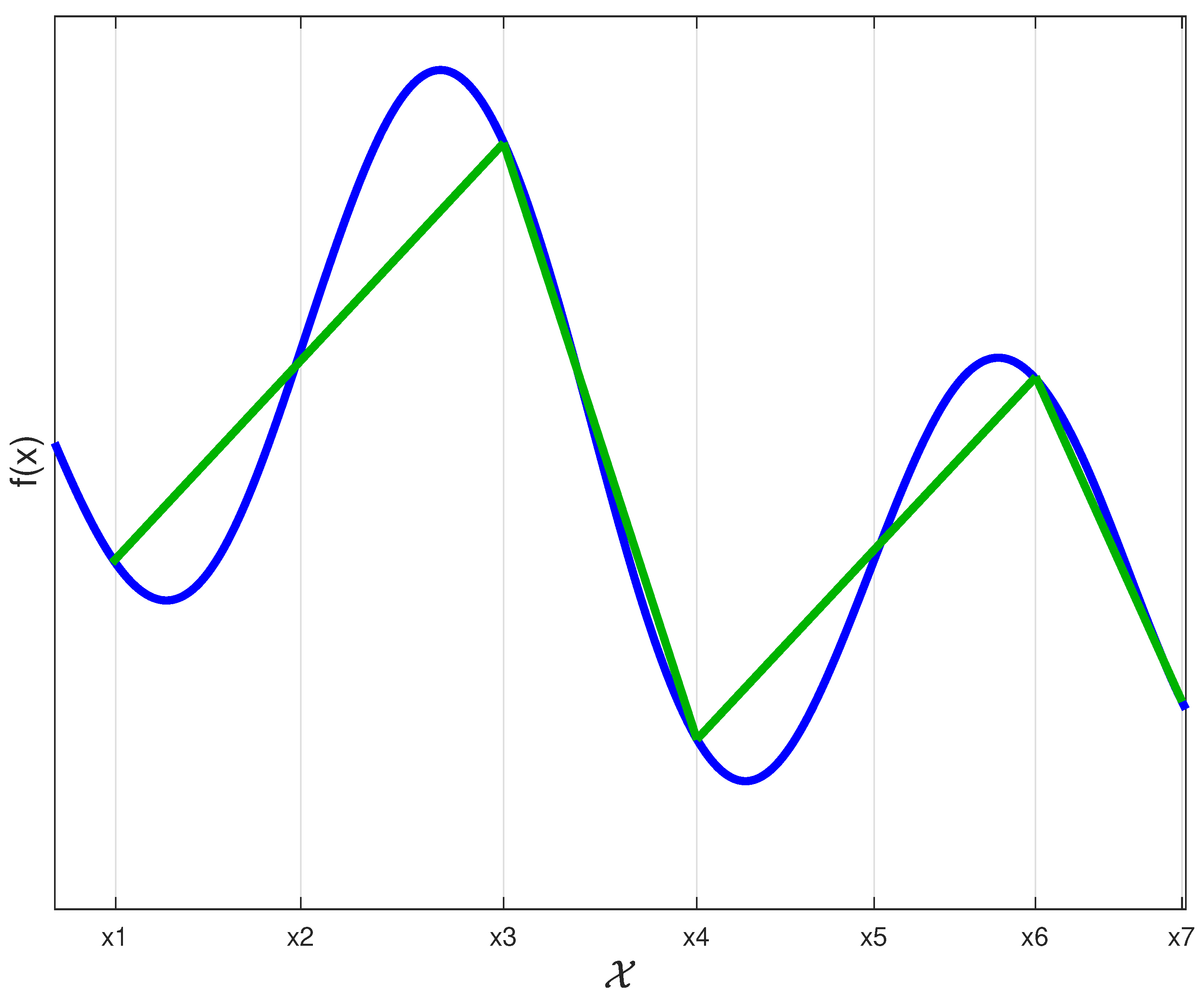
Figure 5 shows an example of a sampling error when ${\Delta }_i=x_{i+1}-x_i=\Delta$, i.e., uniform sampling. It can be seen that the approximation error increases with the curvature (second derivative) of the function.

Figure 5. It can be seen that the uniform sampling error increases with the magnitude of the curvature.

The curvature of the function $f\left(x\right)$ is formally defined as

$$\begin{array}{c}\hfill C\left(x\right)=\frac{d^{2}f\left(x\right)}{d{x}^2}\end{array}$$

(55)

Let us assume, without loss of generality, that the sign of curvature changes at $k(\ge 1)$ points and denote these k values as $x_{i_1},x_{i_2},\cdots ,x_{i_k}$. That is, $x_i=\{x_{i_1},x_{i_2},\cdots ,x_{i_k}\}$ satisfies

$$\begin{array}{c}\hfill C\left(x_{i_j}\right)={\left.\frac{d^{2}f\left(x\right)}{d{x}^2}\right|}_{x=x_{i_j}}=0,j=1,2,\dots ,k\end{array}$$

(56)

These k values of $x_i$ are denoted as the ‘inflection points’ or ‘critical points’ from now on. The nature of the curve significantly changes at critical points. When the function changes from convex to concave, the sign of the curvature changes from positive to negative and vice versa; hence, one support point is assigned to each of the k critical points. Moreover, one support point is assigned, each at the start and end of the interval $[a,b]$, i.e., out of the n available support points, $k+2$ points—$x_1=a$, $x_n=b$ and the k values of $x_i$—are preassigned. These $k+2$ points are denoted as the ‘preassigned points’ from now on. This leaves us with $n-k-2$ points to be assigned to $k+1$ segments created by the k inflection points. The selection of these samples consists of the following two steps:

(a)

Find the number of support points to be allocated to each of the $k+1$ sections created by the k inflection points.

(b)

Place the support points in each section.

The following notations are used to describe these approaches:

$$\begin{array}{cc}\hfill r& \hfill =⌊\frac{n-k-2}{k+1}⌋\hfill \end{array}$$

(57)

$$\begin{array}{cc}\hfill m& \hfill =mod\left(\frac{n-k-2}{k+1}\right)\hfill \end{array}$$

(58)

where $\lfloor ·\rfloor$ denotes the floor operation and $mod\left(·\right)$ denotes the modulus operation. Here, one can see that

$$\begin{array}{c}\hfill n-k-2=r(k+1)+m\end{array}$$

(59)

The absolute area of the curvature in each of the $k+1$ sections is defined as

$$\begin{array}{c}\hfill A_j={\int }_{x_{i_j}}^{x_{i_{j+1}}}\left|C\left(x\right)\right|dxj=0,1,\dots ,k\end{array}$$

(60)

where $x_{i_0}=a$, $x_{i_{k+1}}=b,$ and $x_{i_1},x_{i_2},\dots ,x_{i_k}$ are defined according to (56).

Remark 2.

$x_{i_0}=a$ and $x_{i_{k+1}}=b$ are not the critical points.

Next, an approach is described to fulfill steps (a) and (b).

(a) Number of support points:

• Each section receives r support points.
• The remaining m support points are allocated as follows:

If $m>3$, the m support points are assigned to section j such that

$$\begin{array}{c}\hfill A_j>A_i\forall i=\{0,1,\dots ,k\},i\ne j\end{array}$$

(61)

Else/If $m>3$ and m is even, $m/2$ support points are assigned to each of section $j_1$ and section $j_2$ such that

$$\begin{array}{c}\hfill A_{j_1},A_{j_2}>A_i\forall i=\{0,1,\dots ,k\},i\ne j_1,i\ne j_2\end{array}$$

(62)

Else/If $m>3$ and m is odd, $\lceil m/2\rceil$ support points are assigned to section $j_1$ such that

$$\begin{array}{c}\hfill A_{j_1}>A_i\forall i=\{0,1,\dots ,k\},i\ne j_1\end{array}$$

(63)

$\lfloor m/2\rfloor$ support points are assigned to section $j_2$ such that

$$\begin{array}{c}\hfill A_{j_2}>A_i\forall i=\{0,1,\dots ,k\},i\ne j_1,i\ne j_2\end{array}$$

(64)

(b) Placement of support points: Once the number of points in each section is allocated, the points in each section are then placed equidistantly within that section. Let us assume that section j, which is bounded by $x_{i_j}$ and $x_{i_{j+1}}$, was assigned L support points. The location of these L support points can be written as

$$\begin{array}{c}\hfill x_l=x_{i_j}+d\ast l,l=1,2,\dots ,L\end{array}$$

(65)

where

$$\begin{array}{c}\hfill d=\frac{x_{i_{j+1}}-x_{i_j}}{L+1}\end{array}$$

(66)

where the distance in each section is determined by the difference between the preassigned points of that section divided by the total number of points plus one of that section.

5. Model Selection Metrics

The OCV–SOC modeling approaches described in Section 3 are designed to minimize the mean square error. In this section, several other error metrics are introduced to assess the performance of an OCV–SOC model. A good model is expected to perform well across all error metrics introduced in this section. It is also important that an OCV model consists of as few parameters as possible. Several information theoretic metrics are introduced in this section to collectively evaluate models based on their error performance and the number of parameters that they require. In addition to this, there are other practical selection criteria for an OCV–SOC model: computational complexity, memory requirement, and numerical stability. This section provides brief discussions of these models’ selection criteria.

5.1. OCV Prediction Error

The following four error metrics can be used to evaluate OCV models.

• Best-fit.

  $$\begin{array}{c}\hfill \mathrm{BF}(\%)=\left(1-\frac{∥\widehat{\mathbf{v}}-\mathbf{v}∥}{∥\mathbf{v}-\overline{\mathbf{v}}∥}\right)\times 100\end{array}$$

  (67)
• $R^2$ fit.

  $$\begin{array}{ccc}\hfill {\mathrm{R}}^2(\%)& =& \hfill \left(1-\frac{{∥\widehat{\mathbf{v}}-\mathbf{v}∥}^2}{{∥\mathbf{v}-\overline{\mathbf{v}})∥}^2}\right)\times 100\hfill \end{array}$$

  (68)
• Max-error.

  $$\begin{array}{c}\hfill \mathrm{ME}=\underset{i}{max}\left\{\left|{\mathbf{v}}_i-{\widehat{\mathbf{v}}}_i\right|\right\}\end{array}$$

  (69)
• Root mean square error (RMSE).

  $$\begin{array}{c}\hfill \mathrm{RMSE}=\frac{∥\mathbf{v}-\widehat{\mathbf{v}}∥}{\sqrt{N-M}}\mathrm{or}\sqrt{MSE}\end{array}$$

  (70)

  where N is the number of data points, M is the number of parameters, $\widehat{\mathbf{v}}$ is the predicted value of v using the estimated parameters, for example, for linear models

  $$\begin{array}{c}\hfill \widehat{\mathbf{v}}=\mathbf{P}\widehat{\mathbf{k}}\end{array}$$

  (71)

  and

  $$\begin{array}{c}\hfill \overline{\mathbf{v}}=\frac{1}{N}\sum _{i=1}^N\widehat{\mathbf{v}}\left(i\right)\end{array}$$

  (72)

The best-fit and ${\mathrm{R}}^2$ fit metrics lie between 0 and 1; the higher the value, the better the model. For max-error and RMSE, the lower the value, the better the model. Table 4 contains the values for the four model prediction metrics computed for all models reviewed in Section 3.

Table 4. OCV Prediction errors.

Model	BF	${\mathbf{R}}^2$	ME	RMSE
(2)	80.7150	96.2809	0.6156	0.0533
(3)	69.0215	90.4033	0.2972	0.0856
(4)	84.3122	97.5389	0.5181	0.0433
(5)	90.3010	99.0593	0.3453	0.0268
(6)	96.1031	99.8481	0.1026	0.0108
(7)	92.6999	99.4671	0.2532	0.0202
(8)	94.2150	99.6653	0.4106	0.0160
(10)	94.4633	99.6934	0.1188	0.0153
(11)	85.9646	98.0301	0.4624	0.0388
(12)	83.9417	97.4213	0.5144	0.0444
(13)	83.6839	97.3379	0.5246	0.0451
(14)	95.8975	99.8317	0.1191	0.0113
(15)	82.4227	96.9104	0.5648	0.0486
(65)	97.1593	99.9193	0.0640	0.0078

5.2. Model Evaluation Metrics

Model evaluation metrics consider the trade-off between the number of model parameters and the number of data points. The following four metrics are important ones.

• Akaike’s Information Criterion-1 If the models are fitted using least squares, then [45] suggests the following analog of AIC:

  $$\begin{array}{c}\hfill \mathrm{AIC}=Nln\left(\frac{S_2}{N}\right)+2\left(M+1\right)\end{array}$$

  (73)

  where

  $$\begin{array}{ccc}\hfill S_2& =& \hfill \sum _{i=1}^N{\mathbf{e}}_i^2\hfill \end{array}$$

  (74)

  with

  $$\begin{array}{ccc}& \mathbf{e}=& \hfill \mathbf{v}-\widehat{\mathbf{v}}\hfill \end{array}$$

  (75)
  In the above, $S_2$ is the sum of the squares of errors (SSE), ${\mathbf{e}}_i$ is the ith element of the residual vector e, and M is the number of parameters in the OCV model. The better the model, the lower the AIC.
• Akaike’s Information Criterion-2 The second version of AIC, given below, is useful when $\mathrm{when}N>>M$

  $$\begin{array}{c}\hfill \mathrm{AIC}2=ln\left[{\mathcal{L}}_f\left(1+\frac{2p}{N}\right)\right]\end{array}$$

  (76)

  where the loss function is defined as

  $$\begin{array}{c}\hfill {\mathcal{L}}_f=\frac{{\mathbf{e}}^T\mathbf{e}}{N}\end{array}$$

  (77)
• Akaike’s final prediction error

  $$\begin{array}{c}\hfill \mathrm{FPE}={\mathcal{L}}_f\left[\frac{1+\frac{M}{N}}{1-\frac{M}{N}}\right]\end{array}$$

  (78)
• Bayesian Information Criterion The derivation of BIC assumes equal priors on each model and noninformative priors on the parameters, given each model. The goal of the BIC is to find the best (i.e., highest posterior probability) model for prediction.

  $$\begin{array}{c}\hfill \mathrm{BIC}=2\left(L_N\right)+\left(M+1\right)lnN\end{array}$$

  (79)
  The negative log-likelihood given the pdf of the residuals (assuming normal or Gaussian) conditioned on the parameters k and the s.d. of residuals $\sigma$ is given by

  $$\begin{array}{c}\hfill L_N=-ln\left\{L(\mathbf{k};\mathbf{e})\right\}=\sum _{i=1}^N\left\{\left(\frac{e_i^2}{2{\sigma }^2}\right)+0.5ln\left(2\pi {\sigma }^2\right)\right\}\end{array}$$

  (80)

  where $L_N$ is the negative log-likelihood, L is the likelihood, k is the parameter vector which minimizes $L_N$, and $\sigma$ is the s.d. of the residuals e.
• Minimum description length

  $$\begin{array}{c}\hfill \mathrm{MDL}={\mathcal{L}}_f\left[1+\frac{MlnN}{N}\right]\end{array}$$

  (81)

Table 5 summarizes the five model evaluation metrics computed for all models reviewed in Section 3.

Table 5. Model evaluation metrics.

Model	AIC (${\mathit{e}}^3$)	AIC2	FPE (${\mathit{e}}^{-3}$)	BIC (${\mathit{e}}^3$)	MDL (${\mathit{e}}^{-3}$)
(2)	−2.1841	−5.8644	2.8403	−11.2449	2.8545
(3)	−1.8310	−4.9165	7.3290	−7.7138	7.3656
(4)	−2.3377	−6.2773	1.8805	−12.7746	1.8931
(5)	−2.6955	−7.2390	0.7196	−16.3406	0.7268
(6)	−3.3743	−9.0627	0.1163	−23.1092	0.1181
(7)	−2.9070	−7.8073	0.4079	−18.4492	0.4126
(8)	−3.0803	−8.2725	0.2561	−20.1822	0.2591
(10)	−3.1130	−8.3602	0.2346	−20.5090	0.2374
(11)	−2.4204	−6.4999	1.5060	−13.5956	1.5186
(12)	−2.3197	−6.2306	1.9736	−12.5761	1.9966
(13)	−2.3080	−6.1987	2.0364	−12.4657	2.0567
(14)	−3.3353	−8.9599	0.1292	−22.7015	0.1317
(15)	−2.2518	−6.0498	2.3684	−11.8781	2.4077
(65)	−3.6108	−9.7014	0.0617	−25.4266	0.0633

5.3. Computational Complexity

The OCV–SOC model, once created, is used by the BMS to estimate the SOC of the battery. That is, given the OCV, the BMS needs to use the OCV–SOC model parameters to compute the SOC. For most of the higher-order models, SOC estimation becomes a root-finding problem. For the Unnewehr linear model (2), SOC estimation becomes a closed-form equation, i.e.,

$$\begin{array}{c}\hfill \widehat{s}=\frac{z_v-k_0}{k_1}\end{array}$$

(82)

where $z_v$ is a measure of the open-circuit voltage ($V_{\circ }\left(s\right)$) obtained by the BMS. Similarly, for tabular models, SOC estimation becomes a linear interpolation problem.

Table 6 compares all the models presented in this paper in terms of their required computational complexity to find SOC for a given OCV. It is assumed that in all nonlinear root-finding cases, the bisection method is employed to find the SOC for a given OCV. It is also assumed that the bisection method uses 10 iterations in all cases. It is also assumed that all special functions are approximated for five terms using the Taylor series. The computational complexity shown in Table 6 refers to the number of additions (or subtractions) and multiplications (or divisions) needed to compute the SOC for a given OCV.

Table 6. Computational complexity.

Model	Complexity
(2)	1
(3)	1
(4)	110
(5)	130
(6)	160
(7)	60
(8)	260
(10)	120
(11)	70
(12)	90
(13)	110
(14)	1
(15)	150
(65)	16

5.4. Numerical Stability

Several OCV–SOC models employ functions such as $e^s,ln\left(s\right),sin\left(s\right),$ and $cos\left(s\right).$ The accurate implementation of these functions may require extra computing requirements that may not be affordable in some systems. Approximate implementations may result in errors. For example, the approximate implementation of $ln\left(x\right)$ using Taylor series approximation can be written as

$$\begin{array}{c}\hfill ln(1-x)=-x-\frac{x^2}{2!}-\frac{x^3}{3!}-\frac{x^4}{4!}-\frac{x^5}{5!}-\dots \end{array}$$

(83)

An improved version of the above approximation of natural logarithm through Padé approximation is:

$$\begin{array}{cc}\hfill ln(1-x)& \hfill \approx \frac{0.01812x^5-0.30555x^4-1.30555x^3-2x^2+x}{0.00396x^5-0.11904x^4+0.83333x^3-2.22222x^2+2.5x-1}\hfill \end{array}$$

(84)

$$\begin{array}{cc}\hfill & \hfill \approx \frac{\left(\right(\left(\right(137x-2310)x+9870)x-15120)x+7560)x}{\left(\right(\left(\right(30x-900)x-6300)x-16800)x+18900)x-7560}\hfill \end{array}$$

(85)

which can be implemented efficiently using Horner’s method as follows:

$$\begin{array}{cc}\hfill ln(1-x)& \hfill \approx \frac{\left(\right(\left(\right(137x-2310)x+9870)x-15120)x+7560)x}{\left(\right(\left(\right(30x-900)x-6300)x-16800)x+18900)x-7560}\hfill \end{array}$$

(86)

Figure 6 compares three different implementations of $ln\left(x\right)$: the first one is computed using high-precision computers (Matlab), the second one is computed using (5th-order) Taylor series approximation (83), and the third one is computed using the Padé approximation (86).

Figure 6. Approximate implementation of the natural logarithm.

Figure 6 highlights the importance of numerical stability in the OCV–SOC models. The following two metrics are used to quantify the distortion of an OCV curve in relation to the original, high-precision form.

$$\begin{array}{cc}\hfill \mathrm{KLD}& \hfill =\sum _{i=0}^n{\mathrm{OCV}}_0\left(s_i\right)log\left(\frac{{\mathrm{OCV}}_0\left(s_i\right)}{{\mathrm{OCV}}_1\left(s_i\right)}\right)\hfill \end{array}$$

(87)

$$\begin{array}{cc}\hfill \mathrm{Cos}\mathrm{D}& \hfill =1-\left(\frac{{\sum }_{i=0}^n{\mathrm{OCV}}_0\left(s_i\right){\mathrm{OCV}}_1\left(s_i\right)}{\sqrt{{\sum }_{i=0}^n{\mathrm{OCV}}_0^2\left(s_i\right)}\sqrt{{\sum }_{j=0}^n{\mathrm{OCV}}_1^2\left(s_i\right)}}\right)\hfill \end{array}$$

(88)

where KLD denotes the Kullback–Leiber divergence, CosD denotes the cosine distance, ${\mathrm{OCV}}_0\left(s_i\right)$ denotes the OCV value computed by averaging the collected data for a given (discretized) SOC value $s_i$, and ${\mathrm{OCV}}_1\left(s_i\right)$ denotes the OCV value computed by the model for the same SOC value $s_i$. The KLD and CosD metrics are computed for $n+1$ different SOC values $s_0=0,s_1=1/n,s_2=2/n,\dots ,s_n=1$ spanning the entire SOC range [0, 1]. Table 7 summarizes the stability metrics computed for all the models presented in Section 3.

Table 7. Numerical Stability Metrics.

Model	KLD (${\mathit{e}}^{-4}$)	CosD (${\mathit{e}}^{-4}$)
(2)	1.2328	1.0668
(3)	2.4222	2.3736
(4)	0.7993	0.6909
(5)	0.2592	0.2267
(6)	0.0283	0.0283
(7)	0.1367	0.1252
(8)	0.0705	0.0683
(10)	0.0691	0.0709
(11)	0.6226	0.5446
(12)	0.8277	0.7234
(13)	0.8577	0.7485
(14)	0.0253	0.0267
(15)	1.0064	0.8674
(65)	0.0639	0.0572

5.5. System Requirement

Once an OCV model is selected, its parameters need to be stored by the BMS for SOC estimation. In the case of a combined model (5), the parameters $k_0,\dots ,k_4$ need to be stored. These parameters need to be selected in a way that the computational requirement is minimal. For example, consider the following values for the combined model parameters:

$$\begin{array}{c}\hfill \begin{array}{c}\hfill k_0=-3.265420,k_1=-1.090500,k_2=11.109784,\\ \hfill k_3=2.972069,k_4=-6.158655\end{array}\end{array}$$

(89)

The parameters in (89) have six decimal points. The minimum system requirement to process SOC estimation using these parameters can be approximately stated as follows: 4 bits for the whole number, 20 bits for fractional part, and 1 bit for sign, resulting in a total of 25 bits. In order to fit the above parameters to smaller systems, the parameters in (89) need to be rounded. Let us round the parameters to three decimal points:

$$\begin{array}{c}\hfill \begin{array}{c}\hfill k_0=-3.265,k_1=-1.090,k_2=11.110,\\ \hfill k_3=2.972,k_4=-6.159\end{array}\end{array}$$

(90)

The system requirement to process these new sets of parameters in (90) is as follows: 4 bits for the whole number, 10 bits for fractional part, and 1 bit for sign, resulting in a total of 15 bits.

Rounding the OCV parameters may result in SOC estimation errors. Figure 7 shows the effect of rounding in two different linear models. The rounding error is computed relative to the model that had parameters computed using Matlab in a 64-bit system. Figure 8 shows the effect of rounding for a 16-point tabular approximation. It can be noticed from Figure 7 and Figure 8 that the system requirement to achieve a certain level of maximum SOC error (e.g., 1% max. SOC error) varies from one model to another.

Figure 7. The effect of rounding in two different linear models; (a) the Unnewehr and (b) the Shepherd model is shown.

Figure 8. The effect of rounding in the tabular model is shown.

Table 8 summarizes the system requirement for each model presented in Section 3 in terms of the system requirement to maintain the maximum SOC error below 1%.

Table 8. System requirements for OCV parameters.

Model	Parameters	Bits
(2)	$k_0=3.03,k_1=1.40$	12
(3)	$k_0=4.308,k_1=-0.236$	15
(4)	$k_0=3.982,k_1=0.476,k_2=-0.163$	15
(5)	$k_0=-3.265,k_1=-1.091,k_2=11.109,$$k_4=-6.158$	18
(6)	$k_0=-6.62666$, $k_1=157.30292$, $k_2=-26.85899$, $k_3=2.97206$, $k_4=-0.14404$, $k_5=-127.76012$, $k_6=224.59534$, $k_7=-1.84633$	28
(7)	$k_0=-9.8$, $k_1=27.4$, $k_2=-24.9$, $k_3=9$, $k_4=-258.7$	15
(8)	$k_0=3.3522$, $k_1=-0.8747$, $k_2=4.1821$, $k_3=-3.1107$, $k_4=-0.0017$, $k_5=-2.7797e-15$	19
(10)	$k_0=-228496.9$, $k_1=1.3$, $k_2=492748.6$, $k_3=77.6$, $k_4=-264248.5$, $k_5=15$	22
(11)	$k_0=3.833$, $k_1=0.14$, $k_2=0.866$, $k_3=2.822$	15
(12)	$k_0=1.024$, $k_1=-0.355$, $k_2=1.46$, $k_3=4.611$, $k_4=-6.898$, $k_5=4.016$	15
(13)	$a_1=1.308$, $a_2=1.307$, $b_1=1.503$, $b_2=1.505$, $c=-7.140$	15
(14)	$k_0=-47088.413$, $k_1=838478.954$, $k_2=7077351.741$, $k_3=33622853.695$, $k_4=-77439664.427$, $k_5=68415176.728$, $k_6=3058.908$, $k_7=-379949.127$, $k_8=4021098.125$, $k_9=-12820987.612$, $k_{10}=13436120.396$	38
(15)	$a_1=3.3$, $a_2=3.3$, $a_3=1.76$, $b_1=1.14$, $b_2=1.14$, $b_3=2.72$, $c_1=0.14$, $c_2=0.14$, $c_3=2.11$	12
(65)	rounded to 3 decimal points	8

6. Selection of OCV–SOC Model

The selection of the OCV–SOC model in practical situations is based on requirements that are specific to the application. For example, if high SOC estimation accuracy is required, then models with the lowest error metrics (Section 5.1) will be selected. This would imply that the computational and memory requirements are high. Most practical situations demand more than one constraint in model selection. The Borda count is an intuitive method for combining different selection criteria for a compromised selection. The Borda count was originally a voting method in which each voter gives a complete ranking of all possible alternatives. Table 9 ranks the OCV models presented in this paper based on all the selection criteria discussed in Section 5.

Table 9. Model selection metrics rankings.

Model	BF	${\mathbf{R}}^2$	ME	RMSE	AIC	AIC2	FPE	BIC	MDL	KL	CosD	C	SR	Rank
(65)	1	1	1	1	1	1	1	1	1	4	4	4	1	1
(14)	3	3	4	3	3	3	3	3	3	3	1	1	14	2
(6)	2	2	2	2	2	2	2	2	2	13	2	2	13	3
(10)	4	4	3	4	4	4	4	4	4	10	3	3	12	4
(7)	5	5	5	5	6	6	6	6	6	5	5	5	6	5
(5)	6	6	7	6	7	7	7	7	7	11	6	6	10	6
(11)	8	8	9	8	8	8	8	8	8	6	7	7	7	7
(8)	7	7	8	7	5	5	5	5	5	14	14	14	11	8
(4)	9	9	11	9	9	9	9	9	9	8	8	8	5	9
(12)	10	10	10	10	10	10	10	10	10	7	9	9	8	10
(13)	11	11	12	11	11	11	11	11	11	9	10	10	9	11
(15)	12	12	13	12	12	12	12	12	12	12	11	11	3	12
(2)	13	13	14	13	13	13	13	13	13	1	13	13	2	13
(3)	14	14	6	14	14	14	14	14	14	2	12	12	4	14

7. Conclusions

This paper presents an objective review of models used for OCV–SOC characterization in rechargeable batteries. Available OCV–SOC models are categorized into linear, nonlinear, hybrid, and tabular ones. Model parameter estimation strategies are discussed for each case. A comparative analysis of battery OCV–SOC models is presented in terms of various performance indicators. All models were ranked based on selection metrics, such as OCV prediction accuracy, model evaluation metrics, computational complexity, numerical stability, and system requirement. The proposed systematic approach for OCV–SOC model selection is demonstrated using data collected form a commercially available cylindrical Li-ion battery cell.

A BMS designer can use the proposed approach to select a particular OCV–SOC model for implementation. For instance, in miniature electronics, where memory and computational resources are scarce, one may choose to redo Table 9 based only on the system requirement and computational complexity metrics. The model selection approach can also be modified to give more priority for certain constraints. The proposed approach is general enough to incorporate newer OCV–SOC models and other types model selection metrics. Although the proposed approach is demonstrated using data collected from a Li-ion battery, it can also be applied for model selection in other types of rechargeable batteries.

The proposed approach in this paper is demonstrated using data collected form a particular battery. One should keep in mind that the ranking of models presented in this paper is entirely based on this data; the model order may differ for another battery. It must also be kept in mind that the accuracy of an OCV–SOC model depends on how the OCV–SOC characterization data was obtained. There will be slight cell-to-cell variations, and their effect is neither considered nor quantified in this paper. Future works must consider expanding the approach presented in this paper to incorporate an approach to consider cell-to-cell variances.

References

- Mohammadi, F. Lithium-ion battery State-of-Charge estimation based on an improved Coulomb-Counting algorithm and uncertainty evaluation. J. Energy Storage 2022, 48, 104061. [Google Scholar] [CrossRef]
- Krishna, G.; Singh, R.; Gehlot, A.; Akram, S.V.; Priyadarshi, N.; Twala, B. Digital Technology Implementation in Battery-Management Systems for Sustainable Energy Storage: Review, Challenges, and Recommendations. Electronics 2022, 11, 2695. [Google Scholar] [CrossRef]
- Espedal, I.B.; Jinasena, A.; Burheim, O.S.; Lamb, J.J. Current trends for state-of-charge (SoC) estimation in lithium-ion battery electric vehicles. Energies 2021, 14, 3284. [Google Scholar] [CrossRef]
- Movassagh, K.; Raihan, A.; Balasingam, B.; Pattipati, K. A critical look at coulomb counting approach for state of charge estimation in batteries. Energies 2021, 14, 4074. [Google Scholar] [CrossRef]
- Pattipati, B.; Balasingam, B.; Avvari, G.; Pattipati, K.R.; Bar-Shalom, Y. open-circuit voltage characterization of lithium-ion batteries. J. Power Sources 2014, 269, 317–333. [Google Scholar] [CrossRef]
- Szumanowski, A.; Chang, Y. Battery Management System Based on Battery Nonlinear Dynamics Modeling. IEEE Trans. Veh. Technol. 2008, 57, 1425–1432. [Google Scholar] [CrossRef]
- Relan, R.; Firouz, Y.; Vanbeylen, L.; Timmermans, J.M.; Schoukens, J. Nonparametric analysis of the short-term electrical response of li-ion battery cells. In Proceedings of the 2016 Indian Control Conference (ICC), Hyderabad, India, 4–6 January 2016; pp. 1–6. [Google Scholar]
- Ta, K.P.; Newman, J. Proton Intercalation Hysteresis in Charging and Discharging Nickel Hydroxide Electrodes. J. Electrochem. Soc. 1999, 146, 2769–2779. [Google Scholar] [CrossRef]
- Verbrugge, M.; Tate, E. Adaptive State of Charge Algorithm for Nickel Metal Hydride Batteries Including Hysteresis Phenomena. J. Power Sources 2004, 126, 236–249. [Google Scholar] [CrossRef]
- Plett, G.L. Extended Kalman filtering for battery management systems of LiPB-based HEV battery packs: Part 2: Modeling and Identification. J. Power Sources 2004, 134, 262–276. [Google Scholar] [CrossRef]
- Balasingam, B.; Avvari, G.V.; Pattipati, B.; Pattipati, K.R.; Bar-Shalom, Y. A Robust Approach to Battery Fuel Gauging, Part III: State of Charge Tracking. J. Power Sources 2014. submitted. [Google Scholar]
- Hu, Y.; Yurkovich, S.; Guezennec, Y.; Yurkovich, B.J. Electro-thermal battery model identification for automotive applications. J. Power Sources 2011, 196, 449–457. [Google Scholar] [CrossRef]
- Neumann, D.E.; Lichte, S. A Multi-Dimensional Battery Discharge Model with Thermal Feedback Applied to a Lithium-ion Battery Pack. NDIA Ground Vehicle Systems Engineering and Technology Symposium-Modeling & Simulation, Testing and Validation (MSTV) Mini-Symposium. 2011. Available online: http://gvsets.ndia-mich.org/publication.php?documentID=351 (accessed on 15 July 2022).
- Texas Instruments. 2022. Available online: https://www.ti.com/power-management/battery-management/fuel-gauges/products.html (accessed on 15 July 2022).
- Maxim Integrated. 2022. Available online: https://www.maximintegrated.com/en/products/power/battery-management/MAX17263.html (accessed on 15 July 2022).
- Sundaresan, S.; Devabattini, B.; Kumar, P.; Balasingam, B.; Pattipati, K. Tabular open-circuit Voltage modeling of Li-ion Batteries for Robust SOC Estimation. J. Appl. Energy 2022. submitted. [Google Scholar]
- Mostafa, S.; John, E. Reducing power and cycle requirement for fast fourier transform of electrocardiogram signals through low level arithmetic optimizations for cardiac implantable devices. J. Low Power Electron. 2016, 12, 21–29. [Google Scholar] [CrossRef] [PubMed]
- Pevec, D.; Babic, J.; Carvalho, A.; Ghiassi-Farrokhfal, Y.; Ketter, W.; Podobnik, V. Electric Vehicle Range Anxiety: An Obstacle for the Personal Transportation (R)evolution? In Proceedings of the 2019 4th International Conference on Smart and Sustainable Technologies (SpliTech), Split, Croatia, 18–21 June 2019; pp. 1–8. [Google Scholar] [CrossRef]
- Borda, J.D. Mémoire sur les élections au scrutin. In Histoire de l’Academie Royale des Sciences pour 1781 (Paris, 1784); 1784; pp. 657–665. [Google Scholar]
- Engineering Village. 2022. Available online: https://www.engineeringvillage.com/search/quick.url (accessed on 9 September 2022).
- Baccouche, I.; Jemmali, S.; Manai, B.; Omar, N.; Essoukri Ben Amara, N. Improved OCV model of a Li-ion NMC battery for online SOC estimation using the extended Kalman filter. Energies 2017, 10, 764. [Google Scholar] [CrossRef]
- Lazreg, M.B.; Jemmali, S.; Baccouche, I.; Manai, B.; Hamouda, M. Lithium-ion battery pack modeling using accurate OCV model: Application for SoC and SoH estimation. In Proceedings of the 2020 IEEE 4th International Conference on Intelligent Energy and Power Systems (IEPS), Istanbul, Turkey, 7–11 September 2020; pp. 175–179. [Google Scholar]
- Zhang, Q.; Cui, N.; Li, Y.; Duan, B.; Zhang, C. Fractional calculus based modeling of open-circuit voltage of lithium-ion batteries for electric vehicles. J. Energy Storage 2020, 27, 100945. [Google Scholar] [CrossRef]
- Chen, M.; Rincon-Mora, G.A. Accurate electrical battery model capable of predicting runtime and IV performance. IEEE Trans. Energy Convers. 2006, 21, 504–511. [Google Scholar] [CrossRef]
- Essiet, I.O.; Sun, Y. Optimal open-circuit voltage (OCV) model for improved electric vehicle battery state-of-charge in V2G services. Energy Rep. 2021, 7, 4348–4359. [Google Scholar] [CrossRef]
- ThermoAnalytics, I. Battery modeling. Available online: http://www.thermoanalytics.com/docs/batteries.html (accessed on 15 July 2022).
- Zhang, C.; Jiang, J.; Zhang, L.; Liu, S.; Wang, L.; Loh, P.C. A generalized SOC-OCV model for lithium-ion batteries and the SOC estimation for LNMCO battery. Energies 2016, 9, 900. [Google Scholar] [CrossRef]
- Nejad, S.; Gladwin, D.; Stone, D. A systematic review of lumped-parameter equivalent circuit models for real-time estimation of lithium-ion battery states. J. Power Sources 2016, 316, 183–196. [Google Scholar] [CrossRef]
- Elmahdi, F.; Ismail, L.; Noureddine, M. Fitting the OCV–SOC relationship of a battery lithium-ion using genetic algorithm method. In Proceedings of the E3S Web of Conferences. EDP Sciences, Kenitra, Morocco, 25–27 December 2020; Volume 234, p. 00097. [Google Scholar]
- Weng, C.; Sun, J.; Peng, H. A unified open-circuit-voltage model of lithium-ion batteries for state-of-charge estimation and state-of-health monitoring. J. Power Sources 2014, 258, 228–237. [Google Scholar] [CrossRef]
- Yu, Q.; Wan, C.; Li, J.; E, L.; Zhang, X.; Huang, Y.; Liu, T. An open-circuit voltage model fusion method for state of charge estimation of lithium-ion batteries. Energies 2021, 14, 1797. [Google Scholar] [CrossRef]
- Roscher, M.A.; Sauer, D.U. Dynamic electric behavior and open-circuit-voltage modeling of LiFePO4-based lithium ion secondary batteries. J. Power Sources 2011, 196, 331–336. [Google Scholar] [CrossRef]
- He, H.; Zhang, X.; Xiong, R.; Xu, Y.; Guo, H. Online model-based estimation of state-of-charge and open-circuit voltage of lithium-ion batteries in electric vehicles. Energy 2012, 39, 310–318. [Google Scholar] [CrossRef]
- Ren, Z.; Du, C.; Wu, Z.; Shao, J.; Deng, W. A comparative study of the influence of different open-circuit voltage tests on model-based state of charge estimation for lithium-ion batteries. Int. J. Energy Res. 2021, 45, 13692–13711. [Google Scholar] [CrossRef]
- Li, Y.; Guo, H.; Qi, F.; Guo, Z.; Li, M. Comparative study of the influence of open-circuit voltage tests on state of charge online estimation for lithium-ion batteries. IEEE Access 2020, 8, 17535–17547. [Google Scholar] [CrossRef]
- Pan, H.; Lü, Z.; Lin, W.; Li, J.; Chen, L. State of charge estimation of lithium-ion batteries using a grey extended Kalman filter and a novel open-circuit voltage model. Energy 2017, 138, 764–775. [Google Scholar] [CrossRef]
- Balasingam, B.; Avvari, G.; Pattipati, B.; Pattipati, K.; Bar-Shalom, Y. A robust approach to battery fuel gauging, part I: Real time model identification. J. Power Sources 2014, 272, 1142–1153. [Google Scholar] [CrossRef]
- Weng, C.; Sun, J.; Peng, H. An Open-Circuit-Voltage Model of Lithium-Ion Batteries for Effective Incremental Capacity Analysis. In Proceedings of the ASME 2013 Dynamic Systems and Control Conference, Palo Alto, CA, USA, 21 October 2013; p. V001T05A002. [Google Scholar]
- Safari, M.; Delacourt, C. Modeling of a commercial graphite/LiFePO4 cell. J. Electrochem. Soc. 2011, 158, A562–A571. [Google Scholar] [CrossRef]
- Unnewehr, L.E.; Nasar, S.A. Electric Vehicle Technology; John Wiley & Sons: Hoboken, NJ, USA, 1982. [Google Scholar]
- Moore, S.; Ehsani, M. An empirically based electrosource horizon lead-acid battery model. SAE Tech. Pap. 960448 1996, 105, 421–424. [Google Scholar]
- Khattri, K.S. New close form approximations of ln(1+x). Teach. Math. 2009, 12, 7–14. [Google Scholar]
- Pillai, P.; Sundaresan, S.; Kumar, P.; Pattipati, K.; Balasingam, B. OCV test Voltage and Current Data—Samsung-30T INR21700 Battery. Mendeley Data 2022, 1. [Google Scholar] [CrossRef]
- Balasingam, B.; Ahmed, M.; Pattipati, K. Battery management systems—Challenges and some solutions. Energies 2020, 13, 2825. [Google Scholar] [CrossRef]
- Burnham, K.P.; Anderson, D.R. Model Selection and Inference; Springer: Berlin/Heidelberg, Germany, 1998. [Google Scholar]
Publisher’s Note: MDPI stays neutral with regard to jurisdictional claims in published maps and institutional affiliations. |
© 2022 by the authors. Licensee MDPI, Basel, Switzerland. This article is an open access article distributed under the terms and conditions of the Creative Commons Attribution (CC BY) license (https://creativecommons.org/licenses/by/4.0/).