Abstract
The structure of premixed turbulent flames and governing physical mechanisms of the influence of turbulence on premixed burning are often discussed by invoking combustion regime diagrams. In the majority of such diagrams, boundaries of three combustion regimes associated with (i) flame preheat zones broadened locally by turbulent eddies, (ii) reaction zones broadened locally by turbulent eddies, and (iii) local extinction are based on a Karlovitz number , with differently defined being used to demarcate different combustion regimes. The present paper aims to overview different definitions of , comparing them, and suggesting the most appropriate choice of for each combustion regime boundary. Moreover, since certain Karlovitz numbers involve a laminar flame thickness, the influence of complex combustion chemistry on the thickness and, hence, on various and relations between them is explored based on results of complex-chemistry simulations of unperturbed (stationary, planar, and one-dimensional) laminar premixed flames, obtained for various fuels, equivalence ratios, pressures, and unburned gas temperatures.
1. Introduction
Premixed turbulent combustion is an interplay of turbulent fluid motion, molecular heat and mass transfer, hundreds of chemical reactions between thousands of species, and intensive localized heat release. It is a highly non-linear phenomenon that involves processes whose length or time scales can differ by several orders of magnitude. Therefore, the development of a rigorous theory of turbulent flames is not feasible, whereas direct numerical simulations of them are affordable for the simplest flame configurations only.
In such a situation, governing physical mechanisms of premixed turbulent combustion and turbulent flame structure are often discussed by comparing velocity, length, and time scales of the unperturbed laminar flame, i.e., a planar and one-dimensional flame, which propagates at a constant speed and has a constant thickness, with the counterpart scales of turbulence. More specifically, a laminar premixed flame is commonly characterized by its speed , thickness , and time scale . Since turbulence involves a wide spectrum of eddies of significantly different scales, the simplest and widely accepted approach to characterizing the turbulence spectrum consists in adopting both scales of the largest eddies and scales of the smallest eddies. The former includes the rms turbulent velocity , an integral length scale , and a time scale . The latter includes Kolmogorov velocity , length scale , and time scale . Within the framework of the Kolmogorov theory [1,2,3,4], , , and , where is the turbulent Reynolds number and is the kinematic viscosity of unburned reactants. Note that the three scaling laws written above contain unity–order constants, which will be discussed later. Moreover, the entire inertial range of Kolmogorov turbulence is characterized by a single scalar quantity, the mean rate of viscous dissipation of turbulent kinetic energy [1,2,3,4]. Here, is the rate of the strain tensor, is the i-th component of the velocity vector , and the summation convention applies to repeated indexes.
Depending on the relations between the aforementioned flame and turbulence scales, different scenarios of the influence of turbulence on premixed combustion can be assumed. For example, in their classical papers, Damköhler [5] and Shelkin [6] have hypothesized that the influence of turbulence on combustion can be reduced to a wrinkling flame surface (or flame sheet) if the turbulence length scales are much larger than the thickness , i.e., in contemporary terms. Under these conditions, the local flame structure was considered to be similar to the structure of the unperturbed laminar flame, with the bulk burning rate being increased due to wrinkling of the flame surface by turbulent eddies. Today, such a premixed turbulent combustion regime is well established and is called “flamelet regime”, where the word “flamelet” refers to a thin, inherently laminar flame wrinkled and strained by turbulent eddies.
In the opposite limit case of , the influence of turbulence on combustion was hypothesized to be reduced to intensifying mixing [5] within a flame broadened significantly by turbulent eddies [6,7]. The existence of this regime is still under discussion, and this issue will be briefly addressed later.
While the pioneering papers by Damköhler [5] and Shelkin [6] highlighted relations between length scales, over (velocity and time) scales were later used to specify boundaries of the two limit combustion regimes discussed above and to explore other combustion regimes. That research resulted in the appearance of premixed turbulent combustion regime diagrams. Today, such diagrams are widely used in the literature. The first combustion regime diagrams were invented by Bray [8], Barrere [9], Borghi [10,11], Williams [12,13,14], and Peters [15], with a number of modified diagrams being introduced later, e.g., see Refs. [16,17,18,19,20,21,22]. The goal of such diagrams is to speculate what physical mechanisms of the influence of turbulence on combustion are of importance under specific conditions and what structure local reaction zones have under such conditions. The following discussion is restricted to premixed combustion in a turbulent flow characterized by a low Mach number, and almost all such combustion regime diagrams are restricted to considering the influence of turbulence on an adiabatic, single-step-chemistry (i.e., thousands of reactions between hundreds of species are modeled with a single reaction between two reactants), and equidiffusive (i.e., molecular diffusivities of all reactants and products are equal to molecular heat diffusivity of the mixture) flames. Important effects that stem from the influence of combustion-induced thermal expansion on turbulence [23,24,25,26,27], differences in molecular transport coefficients [28], heat losses, and complex combustion chemistry are often beyond the scope of such diagrams. Thus, a typical combustion regime diagram deals with a constant-density single-reaction wave, which passively propagates in turbulence described by the Kolmogorov theory [1,2,3,4].
Moreover, in the classical combustion regime diagrams [8,9,10,11,12,13,14,15], the following simplifications were invoked: (i) all constants in the aforementioned scaling laws were set equal to unity, i.e., , , , and , (ii) all molecular transport coefficients were set equal to the kinematic viscosity of the mixture, and (iii) the laminar flame thickness was evaluated as follows . Under these simplifications,
where the Karlovitz number characterizes a ratio of the flame and Kolmogorov time scales, whereas the Damköhler number involves the time scale of the largest turbulent eddies. Here, a single symbol is adopted to designate various numbers, which are different in a general case, e.g., if . Differences in these numbers will be discussed in Section 3. According to Equation (1), among various non-dimensional characteristics of flame–turbulence interaction, e.g., , etc., only two characteristics are independent. Therefore, typical combustion regime diagrams are 2D planes with different coordinate axes, e.g., and [8], and [9,11,15], and [12], or and [14].
In all the combustion regime diagrams [8,9,10,11,12,13,14,15,16,17,18,19,20,21,22], lines of constant Karlovitz numbers are of particular importance, while different definitions of these numbers are adopted in different diagrams. Equation (1) shows that the same can be obtained by invoking different non-dimensional characteristics of the influence of turbulence on premixed combustion. However, if (i) differences between unity and the aforementioned constants adopted to link small-scale and large-scale turbulence characteristics are taken into account, (ii) Prandtl number , (iii) the thickness is defined using a molecular transport coefficient evaluated inside the flame, i.e., at a higher temperature , etc., none of the equalities in Equation (1) are met. Moreover, in this case, physical mechanisms that are hypothesized to play an important role under conditions of either or , should be associated with different areas of a combustion regime diagram, whereas these areas coincide if Equation (1) holds. While these ambiguities are rarely emphasized in the literature, they should be borne in mind when analyzing published data and, especially, when comparing results reported by different research groups. Accordingly, the present paper aims to summarize the use of differently defined Karlovitz numbers for demarcating combustion regimes. Moreover, the paper aims to discuss the influence of combustion chemistry on the thickness and, consequently, on differences between differently defined Karlovitz numbers. It is worth stressing, however, that the focus of the following discussion will be restricted to the ambiguity of the term “Karlovitz number”, whereas consideration of various regimes of premixed turbulent combustion or boundaries of such regimes is beyond the major scope of the present article, while these issues will briefly be addressed in the following.
In the next section, physical mechanisms whose importance is commonly assessed by invoking criteria of const are discussed. A summary of differently used in the literature is given in Section 3. Effects of complex combustion chemistry on thicknesses of different zones in a laminar premixed flame and, hence, on differently defined Karlovitz numbers are addressed in Section 4, followed by conclusions summarized in Section 5.
2. Combustion Regime Boundaries and Karlovitz Numbers: A Historical Overview
To the best of the authors’ knowledge, Kovasznay [29] was the first who proposed to use a criterion of to characterize the transition from (i) combustion localized to thin inherently laminar flames wrinkled by turbulent eddies (at low values of ) to (ii) chemical reactions distributed in wide zones (at high values of ). Here, designates the transverse Taylor microscale of turbulence and, under the simplifications invoked to arrive at Equation (1), . Kovasznay [29] attributed the transition to the local break-up of laminar flames by turbulence-induced velocity gradients and, following the Kolmogorov theory, adopted to characterize the magnitude of the largest velocity gradients created by the smallest-scale turbulent eddies [2,3,4]. Earlier, the quenching of laminar premixed flames by an external velocity gradient was predicted by Karlovitz et al. [30], and another Karlovitz number was used as a criterion of such quenching in the laminar combustion literature [31]. Here, is the transverse gradient of the -component of the velocity of a laminar flame upstream of a flame.
Later, by theoretically studying the response of twin laminar premixed flames to a strain rate created by two identical counter-flows, Klimov [32] obtained a number of seminal results. In particular, (i) the flame speed can be negative if the strain rate is sufficiently high, and (ii) the flame can be quenched by a higher strain rate, but (iii) the quenching process takes time. Based on these findings, Klimov [32] hypothesized three combustion regimes: (i) combustion localized to thin inherently laminar flames wrinkled by turbulent eddies (at low values of ), (ii) combustion localized to thin reaction zones strongly perturbed by turbulent eddies, with the probability of local combustion extinction being low (if is of unity order), and (iii) intermittency of such reaction zones and reacting (self-igniting) hot volumes appearing due to local combustion quenching by turbulent eddies (if is much larger than unity). The third regime is similar to a turbulent combustion regime hypothesized earlier by Shetinkov [33] and discussed subsequently in his book [34] in a more detailed manner. The reader interested in Shetinkov’s concept is also referred to [35].
Based on the theoretical results obtained by Klimov [32], Williams [36] highlighted the appearance of negative flame speeds in a turbulent flow, which could cause the annihilation of hot spots of burned gas. Due to this mechanism, combustion was hypothesized to be localized to thin inherently laminar flames wrinkled by turbulent eddies only if and a criterion of was adapted [36,37], i.e., Williams [36,37] wrote this criterion in a form of by invoking the assumptions taken to arrive at Equation (1). Subsequently, by introducing a premixed turbulent combustion regime diagram, Williams [13] (i) placed the focus of consideration on the limit cases of and , (ii) did not highlight a constraint of at high , but (iii) noted that an intermediate regime or more than one intermediate regime could exist if .
By referring to the papers by Klimov [32] and Williams [36,37], Bray [8] considered a constraint of to limit the existence of laminar flames in a turbulent flow. Moreover, Bray [8] drew a line of as a boundary of the flamelet combustion regime on a 2D plane but did not specify other combustion regimes on this plane, contrary to subsequent multi-regime diagrams [9,10,11,12,13,14,15,16,17,18,19,20,21,22].
Kovasznay [29], Klimov [32], Williams [12,13,14,36,37], and Bray [8] did not apply the term “Karlovitz number” to turbulent combustion, while Bray [8] introduced a criterion of and used a similar symbol to designate the Karlovitz stretch factor when referring to combustion quenching in laminar flows and to the pioneering study by Karlovitz et al. [30]. To the turbulent combustion literature, the term “Karlovitz flame stretch factor was likely introduced by Abdel-Gayed et al. [38], who discussed that premixed combustion could be quenched by turbulence when
Thus, the authors of Refs. [8,29,32,36,37,38] stressed the importance of the number for characterizing the influence of turbulence on the local flame structure. All these authors agreed that, at , (i) combustion should be localized to thin inherently laminar flames and (ii) an increase in burning rate resulted from an increase in the wrinkled flame surface area, in line with the first Damköhler hypothesis [5]. As far as combustion at a large is concerned, scenarios discussed in the cited papers are different. Kovasznay [29] and Klimov [32] hypothesized a transition to distributed burning due to local combustion quenching. Williams [36] emphasized the annihilation of hot spots of burned gas. Bray [8] highlighted local combustion quenching by velocity gradients and noted that the quenching could play an important role even if was smaller than unity. Abdel-Gayed et al. [38] also highlighted flame quenching by turbulence based mainly on their experimental data obtained from statistically spherical flames expanding in turbulence generated by fans in a closed vessel.
There is another important difference between phenomenological scenarios presented in Refs. [8,13,29,32,36,37,38]. While a constraint of was written in Refs. [8,29,36,37,38], Klimov [32] clearly stated that thin reaction zones could dominate even at significantly larger . Accordingly, Klimov (private communications, 1981–2010) never accepted the term “Klimov-Williams criterion”, which was widely applied to the constraint . Recent experimental and numerical data reviewed elsewhere [22,39,40], as well as experimental [41] and numerical [42,43,44,45,46,47] papers published over the past two years, indicate that inherently laminar flamelets can survive and control statistical characteristics of premixed turbulent flames at large , in line with Klimov’s standpoint. Williams did not highlight the constraint in his book [13] either.
While the studies cited above placed the focus of consideration on the straining of local laminar flames by velocity gradients created by small-scale turbulent eddies, such eddies can also perturb the local flame structure by entering the local flames and intensifying mixing inside them. This mechanism was emphasized in the premixed turbulent combustion regime diagrams by Borghi [10,11] and Peters [15]. Under the simplifications invoked to arrive at Equation (1), the “quenching criterion”, i.e., , occasionally coincides with the “mixing criterion”, i.e., . Therefore, the two criteria simply read . Accordingly, in the majority of premixed turbulent combustion regime diagrams [8,10,11,15,16,17,18,19,20,21,22], the same line plays the most important role and is considered to be (i) a boundary of a regime associated with a substantial probability of local flame quenching and (ii) a boundary of a regime associated with local flames broadened by small-scale turbulent eddies. However, in a general case, the two boundaries should be different, as will be discussed in the next section.
In addition, in many recent diagrams, there is another line of . This line was first drawn by Peters [18,48] to highlight the so-called thin reaction zone regime of premixed turbulent combustion. In this regime, the smallest turbulent eddies are sufficiently small to enter the preheat zones of the local flames, i.e., , but are too large to enter significantly thinner reaction zones of these flames, i.e., . Here, is the reaction zone thickness, and Peters [18,48] assumed that . It is worth remembering that, within the framework of the classical Activation Energy Asymptotics (AEA) theory of laminar premixed flames [49], and the flame speed is controlled by a reaction time scale and molecular heat diffusivity in the reaction zone. Accordingly, penetration of small-scale eddies into thicker preheat zones and intensification of mixing inside these zones can change the local flame structure but weakly affect the local burning rate in a turbulent flow, provided that [50]. Thus, the influence of turbulent eddies on local flames can be different in the flamelet and thin reaction zone regimes. In the former regime, the entire local flames retain their laminar structure, whereas preheat zones are broadened in the latter regime, but the local burning rates retain the laminar values. However, while the division of a laminar premixed flame into a thick preheat zone and a thin reaction zone is fully justified within the framework of the classical AEA theory of single-step-chemistry laminar premixed flames [49], such a division could be disputed for certain complex-chemistry flames. Moreover, for the latter flames, an estimate of appears to be too strong. These two points, which are of importance for accurately specifying the upper boundary of the thin reaction zone regime, will be discussed in Section 4.
3. Differently Defined Karlovitz Numbers
Let us, following common practice [2,3,4], define Kolmogorov length, time, and velocity scales as follows:
Henceforth, all turbulence characteristics are evaluated in unburned gas upstream of a flame if the opposite is not specified.
In homogeneous isotropic turbulence [51],
Here, is a constant, which is often assumed to be of unity order, but its exact value is not known a priori. In the simplest case of homogeneous isotropic turbulence, an increase in with decreasing Reynolds number is well documented in Direct Numerical Simulation (DNS) studies [52,53], with the effect being strongly pronounced at . These DNS data also indicate that tends to a finite constant value (about 0.5) as , but this asymptotic value depends on “details of forcing at low wavenumbers” [52]. Burattini et al. [54] summarized experimental data on , obtained by themselves and by other research groups from different flows under different conditions. Figure 1 in the cited paper shows that measured at approximately the same (in a range of ) in different flows varies from 0.5 to 2.6, with a dependence of on being either weakly pronounced or even increasing in some of the experiments. Accordingly, Burattini et al. [54] have concluded that “a universal value for” “is not tenable” and “the flow type and initial conditions (for any given flow type) seem to have a persistent influence even in the fully developed region of the flow”. Recently, Vassilicos [55] has argued that in spatially decaying turbulent flows (e.g., flows behind various grids or wakes), there exists a significant nonequilibrium region, where is roughly proportional to a ratio of an inlet Reynolds number, which is constant for each specific flow, to the local turbulent Reynolds number, which could vary as the turbulence decays. Accordingly, data measured at different distances from a grid or wake could show an increase in with a decreasing turbulent Reynolds number.
In the combustion literature, the values of are even more scattered because different methods are adopted to evaluate the length scale , with the chosen method being poorly described in many papers. For instance, if the length scale is evaluated as follows , the constant . This value of was adopted in some experimental [56,57,58,59] and DNS [60,61,62,63,64,65] studies. If [51,66,67], where designates the mean value of turbulent kinetic energy, then . If designates longitudinal or transverse integral length scale, the “constant” is poorly known and is not constant [51,52,53,54,55]. By referring to the results of their measurements, Abdel-Gayed et al. [38] have set , which is equivalent to in Equation (3). In commercial CFD codes, the default value of is commonly equal to , i.e., if . Steinberg et al. [27] recommended in . Accordingly, , because . These examples show that the values of can differ by a factor as large as 30. In an anisotropic turbulent flow associated with a typical burner, evaluation of is even more difficult.
Using Equations (2) and (3), the following relations could be obtained:
Subsequently, substituting Equations (3) and (4) into Equation (1) and introducing a flame-thickness factor (or a flame counterpart of Reynolds number):
we arrive at:
Various parts of Equation (6) were earlier adopted to calculate a Karlovitz number. For instance, Abdel-Gayed et al. [38] have introduced a Karlovitz number as follows:
by setting in Equation (4) and assuming that . Since that seminal work, Equation (7) was adopted in many papers. In certain papers, the second equality in Equation (7) was not invoked, and the Karlovitz number was evaluated using measured values of rms turbulent velocity and Taylor microscale [56,68].
In other experimental papers, e.g., see Ref. [57], these measured values were adopted to calculate a differently defined Karlovitz number:
The same Karlovitz number written in the form of is sometimes used in DNS papers, e.g., see Ref. [66], where the dissipation rate is directly evaluated.
Conditions of experiments are often characterized by setting both and [69,70,71], i.e., by invoking the following number:
The same number is widely used in DNS [63,72,73,74] and review [22,39] articles also. This number may be interpreted to characterize a ratio of the dissipation rate to its flame counterpart , i.e., .
In other DNS papers [61,65,75,76], the factor is retained, i.e., the DNS conditions are characterized with:
Finally, many authors evaluate one more Karlovitz number using a ratio of a laminar flame thickness and Kolmogorov length scale [58,77,78,79,80,81,82], i.e.,
The above brief review shows that several differently defined Karlovitz numbers are adopted in the literature. It is worth stressing that this ambiguity is even greater because differently defined laminar flame thicknesses could be substituted in each of Equations (7)–(11), e.g., (i) , (ii) and is inversely proportional to Prandtl number in this case, (iii) , where designates molecular diffusivity of deficient reactant, and is inversely proportional to Schmidt number in this case, (iv) each of the aforementioned molecular transport coefficients could be taken at an intermediate temperature, etc.
Based on the historical overview provided in Section 2, the use of the ratio as a Karlovitz number appears to be the most appropriate choice. While application of Equations (7) and (9) or (10) seems to be easier, the Taylor microscale can be evaluated in the state-of-the-art measurements and DNSs either directly or indirectly (e.g., , where the dissipation rate is either measured or sampled from DNS data). In the following,
and Equations (6) and (8)–(11) read:
It is also worth noting that (i) DNS data by Girimaji et al. [83,84] show that the mean strain rate in a turbulent flow is about , in line with the above relation between and , and (ii) difference in and can reach an order of magnitude depending on the value of .
The use of the term “Karlovitz number”, i.e., , defined by Equation (11), as a criterion of penetration of the smallest-scale turbulent eddies into flame preheat zones does not seem to be historically justified because Karlovitz did not highlight this physical mechanism. Moreover, the criteria of and are different in a general case (see Equation (13)), where can be large, as discussed in the next section. Therefore, another name for a ratio of as a boundary of broadened preheat zone regime appears to be more appropriate both from the historical and fundamental perspectives.
The same comments hold for a criterion of , introduced by Peters [18,48]. Relation between the number or and or depends on a ratio of , which, in its turn, depends on mixture composition, pressure, and temperature, as discussed in the next section.
4. Preheat and Reaction Zone Thicknesses of Complex-Chemistry Flames
To evaluate and , numerical simulations of unperturbed, complex-chemistry, adiabatic, laminar premixed flames were performed by running PREMIX code [85] of CHEMKIN-II software package [86] to numerically integrate stationary, one-dimensional transport equations for species mass fractions and energy, supplemented with the ideal gas state equation and the continuity equation. Thermo-diffusion and multi-species diffusion options were activated for H2, CH4, and C3H8. For methane, the GRI mechanism [87] (53 species and 325 reversible reactions) was adopted. Hydrogen, propane, and n-heptane–air flames were simulated, invoking chemical mechanisms by Konnov [88] (15 species and 75 reversible reactions), Chaos et al. [89] (117 species and 755 reversible reactions), and Huang et al. [90] (114 species and 632 reversible reactions), respectively.
Figure 1, Figure 2, Figure 3 and Figure 4 show profiles of the temperature-based combustion progress variable (solid red lines), fuel-based combustion progress variable (black dashed lines), fuel consumption rate (FCR) (blue dotted-dashed lines), and heat release rate (HRR) (magenta or violet double-dashed-dotted lines) obtained from complex-chemistry lean, stoichiometric, and rich hydrogen–air (Figure 1), methane–air (Figure 2), propane–air (Figure 3), and n-heptane–air (Figure 4) unperturbed laminar flames under room conditions. Here, designates fuel mole fraction, subscripts u and b refer to unburned reactants and burned products, respectively, and the rates are normalized using their peak values in the flame. Differently defined flame thicknesses obtained using these profiles are reported in Figure 5.
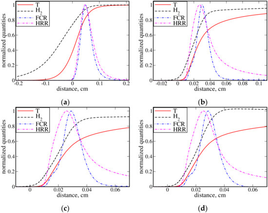
Figure 1.
Profiles of , , fuel consumption rate, and heat release rate, normalized using their peak values. The profiles have been obtained from unperturbed hydrogen–air premixed flames characterized by different equivalence ratios: (a) , (b) , (c) , and (d) .
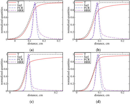
Figure 2.
Profiles of , , fuel consumption rate, and heat release rate, normalized using their peak values. The profiles have been obtained from unperturbed methane–air premixed flames characterized by different equivalence ratios: (a) , (b) , (c) , and (d) .
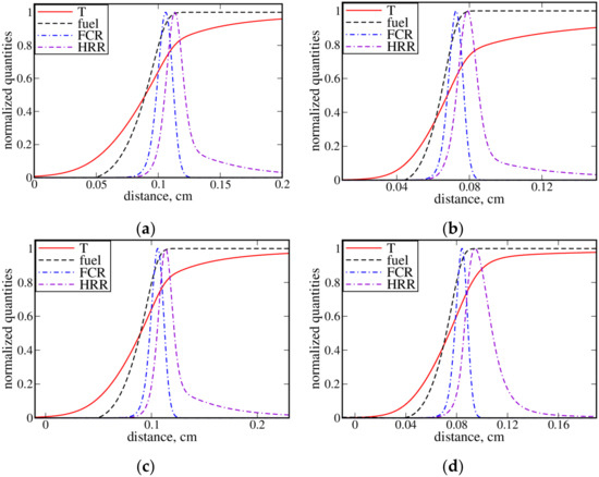
Figure 3.
Profiles of , , fuel consumption rate, and heat release rate, normalized using their peak values. The profiles have been obtained from unperturbed propane–air premixed flames characterized by different equivalence ratios: (a) , (b) , (c) , and (d) .
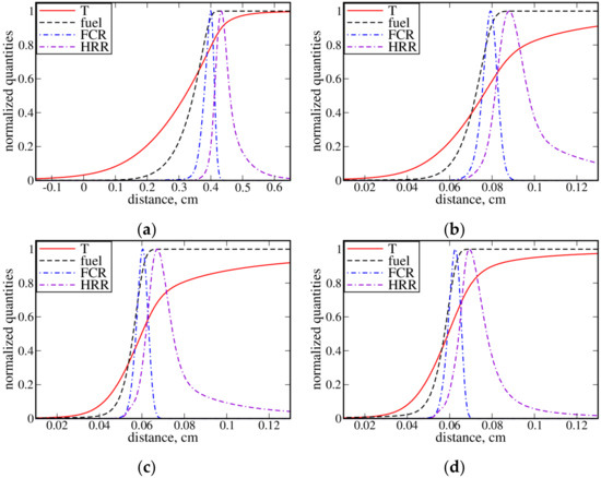
Figure 4.
Profiles of , , fuel consumption rate, and heat release rate, normalized using their peak values. The profiles have been obtained from unperturbed n-heptane–air premixed flames characterized by different equivalence ratios: (a) , (b) , (c) , and (d) .
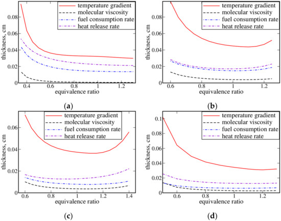
Figure 5.
Dependencies of differently defined laminar flame thicknesses on the equivalence ratio, computed for (a) H2–air, (b) CH4–air, (c) C3H8–air, and (d) n-C7H16–air mixtures under room conditions.
In all studied flames (maybe, with the exception of the leanest n-heptane–air flame, see Figure 4a), the laminar flame thickness is controlled by the maximal temperature gradient and evaluated as follows:
seems to be quite comparable with the reaction zone thickness or equal to the halfwidth of the fuel consumption rate profile or the heat release rate profile, respectively. In the H2–air mixtures, with the exception of the leanest one, see Figure 1a, the thickness seems to be close to , cf. curves plotted in red solid and magenta double-dashed-dotted lines in Figure 1b–d. Moreover, in these flames, there are wide radical recombination zones, where the temperature grows gradually due to heat release in slow three-molecular reactions between radicals [91]. Thus, in these three moderately lean, stoichiometric, and moderately rich H2–air flames, reaction zones are not significantly thinner than other (preheat and radical recombination) zones, and the separation of broadened preheat zone and broadened reaction zone regimes of premixed turbulent combustion does not seem to be fundamentally justified. Therefore, a criterion of , introduced by Peters [18,48] as a boundary of thin reaction zone regime, appears to be irrelevant to moderately lean, stoichiometric, and moderately rich H2–air flames.
In the leanest H2–air flame, see Figure 1a, fuel consumption and heat release zones are a little thinner than preheat zone. While difference in or and a laminar flame thickness is substantially increased if the latter thickness is evaluated as follows:
This measure of laminar flame thickness is seldom used in the literature, contrary to Equation (14). Here, designates fuel mass fraction and is significantly larger than the thickness defined by Equation (14) because the molecular diffusivity of hydrogen is much larger than the molecular heat diffusivity in a lean H2–air mixture.
In hydrocarbon–air flames, see Figure 2, Figure 3 and Figure 4, the thickness is distinctly larger than or , but the difference seems to be really large in the leanest n-heptane–air flame only, see Figure 4a. Note that the difference is significantly reduced if the thickness of propane–air or n-heptane–air flame is quantified with defined by Equation (15).
Figure 5 further emphasizes that in hydrogen–air or paraffin–air complex-chemistry laminar premixed flames under room conditions, differences between thicknesses of preheating zones, see solid red lines, and reaction zones, see blue and violet dotted-dashed lines, are sufficiently small. As shown in Figure 6, such differences are substantially less than an order of magnitude. More specifically, is close to in the studied H2–air mixtures, see red circles, with a ratio of (i) being slowly increased with decreasing the equivalence ratio and (ii) reaching two at . In the studied paraffin–air flames, the ratio is slightly above two in rich mixtures, increases moderately with decreasing the equivalence ratio, is close to four in the richest methane–air and propane-flames and is about 5.5 in the richest n-heptane–air flame.
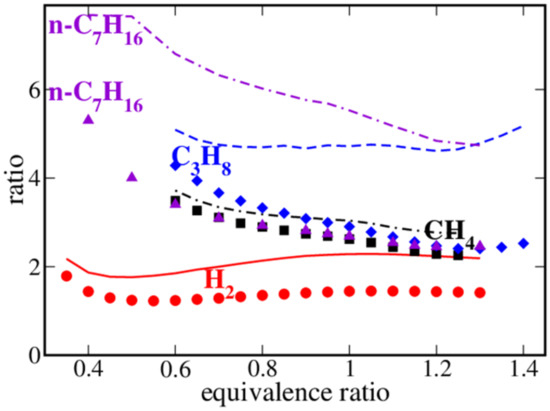
Figure 6.
Dependencies of the ratios (lines) and (symbols) calculated for various fuels specified in legends.
All in all, Figure 1, Figure 2, Figure 3, Figure 4, Figure 5 and Figure 6 do show that a factor of 0.1 in the criterion , considered to demarcate thin reaction zone regime [18,48] on a premixed turbulent combustion regime diagram, is too small for complex-chemistry flames. Moreover, for the vast majority of the studied mixtures, , thus, putting into question the foundation of the concept of a thin reaction zone (especially for hydrogen–air flames, where ). Under room conditions, such a concept appears to deserve consideration for very lean mixtures of heavy paraffin and air only. One may note that , cf. symbols and lines in Figure 6, because a fuel consumption rate zone is thinner than a heat release zone, cf. curves plotted in blue and violet dotted-dashed lines, respectively, in Figure 5. However, penetration of small-scale turbulent eddies into a thicker heat release zone is sufficient to claim that the boundary of the discussed regime is crossed. Therefore, the boundaries of regimes of broadened preheat zones and broadened reaction zones are so close that the separation of the two regimes does not seem to be fundamentally justified under room conditions. Figure 7 and similar results obtained for (not shown for brevity) indicate that this separation is not fundamentally justified under elevated pressures and temperatures either.
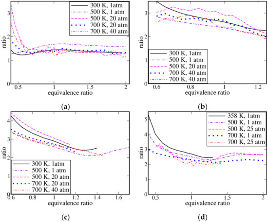
Figure 7.
Dependencies of the ratio on the equivalence ratio, calculated for (a) H2, (b) CH4, (c) C3H8, and (d) n-C7H16, calculated for various pressures and unburned gas temperatures , specified in legends.
Dependencies of the factor on the equivalence ratio, calculated for various fuels under different pressures and unburned gas temperatures are reported in Figure 8. These numerical results indicate that the factor (i) is significantly larger than unity, (ii) is very large for near stoichiometric and moderately rich hydrogen–air mixtures, (iii) depends on the equivalence ratio, (iv) is increased by the unburned gas temperature, and (v) is decreased with increasing pressure. Therefore, the number , defined by Equation (11) and widely used as a criterion of penetration of the smallest-scale turbulent eddies into flame preheat zones, is not equal to the Karlovitz number , defined by Equation (12) and adopted as a criterion of local combustion quenching. Consequently, if the influence of complex combustion chemistry on the laminar flame thickness is taken into account, the use of a single line of as a boundary of (a) broadened preheat zone regime, and (b) regime associated with local combustion quenching is not justified. In other words, the single line , drawn in many combustion regime diagrams, should be split into two different lines. As is significantly larger than unity, the boundary of the former (broadened preheat zone regime) is associated with less intense turbulence (a lower Karlovitz number) when compared to the boundary of the latter regime, see Equation (13). Moreover, distance (in a 2D combustion regime diagram) between the boundaries of the two regimes should depend on fuel formula, equivalence ratio, unburned gas temperature, and pressure, which affect the factor .
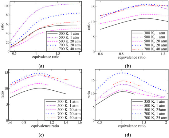
Figure 8.
Dependencies of the factor on the equivalence ratio, calculated for (a) H2, (b) CH4, (c) C3H8, and (d) n-C7H16, calculated for various pressures and unburned gas temperatures , specified in legends.
5. Concluding Remarks
First, while the numbers (i) or (ii) , which are widely adopted to demarcate (i) a combustion regime associated with the importance of local flame quenching by small-scale turbulent eddies or (ii) a combustion regime associated with broadening of preheating zones by small-scale turbulent eddies, respectively, are both proportional to the same , the critical values of the two numbers, used to demarcate the combustion regimes, are significantly different in complex-chemistry flames. More specifically, a constraint of should be reached at a substantially lower when compared to a constraint of . Moreover, a ratio of the two numbers, and , depends on fuel formula, equivalence ratio, unburned gas temperature, and pressure. In particular, the ratio of these numbers can be very large in moderately lean, stoichiometric, or rich hydrogen–air mixtures, especially at elevated unburned gas temperatures.
The use of Kolmogorov time and length scales in the discussed constraints can be disputed by noting that Kolmogorov eddies rapidly disappear and, consequently, cannot substantially affect a premixed flame during the eddy lifetime. For instance, following Klimov [32], the criterion of could be changed to . Moreover, based on results of numerical [92,93] and experimental [94] studies of vortex filaments (worms or tubes) in incompressible turbulence, the smallest eddy length scale was argued to be larger than by a factor of about 8. We may also note that experimental data analyzed by Monin and Yaglom ([2], Figure 77) show that the highest rate of dissipation of turbulent energy is also localized at a length scale of about . If this smallest length scale, which was already used in combustion research [27,95], is compared with , then, the classical criterion of , should be changed to , where can be as large as 64. These simple reasoning could explain the utility of the flamelet paradigm even at high Karlovitz numbers, which (utility) was emphasized in recent review articles [22,39,40], as well as in subsequent experimental [41] and numerical [42,43,44,45,46,47] papers. In any case, criteria of local flame broadening, i.e., , and local flame quenching, i.e., , should be different in a general case.
Second, numerical simulations of complex chemistry laminar premixed flames do not warrant separation of a thick preheat zone and a much thinner reaction zone, especially in moderately lean, stoichiometric, and rich hydrogen–air mixtures. Such separation could be acceptable for lean mixtures of heavy paraffin with air, but the ratio of the two thicknesses is significantly less than 10, even in this case. Nevertheless, recent experimental and numerical studies reviewed elsewhere [22,39,40] do show that the reaction zone can retain its (laminar flame) thickness even if turbulence is sufficiently intense to significantly broaden preheating zones. This apparent inconsistency (comparable thicknesses of preheating and reaction zones in laminar flames and well-pronounced broadening of the former zone in certain turbulent flames) could be attributed to the rapid disappearance of the smallest eddies in thick preheat zones due to thermal expansion and a significant increase in the mixture viscosity with the temperature, e.g., see Ref. [96]. DNS data by Bobbitt et al. [97] and by Apsden [98] do indicate that an increase in with the temperature significantly affects the evolution of enstrophy in premixed flames. While recent experiments by Wabel et al. [99] did not show substantial variations in the local turbulent kinetic energy within broadened preheat zones, an increase in the length scale of turbulent eddies conditioned to such zones, was reported in the cited paper, thus, implying a decrease in the local turbulent strain rates. While the discussed hypothesis definitely requires further assessment, it is worth stressing already now that, if confirmed, the hypothesis challenges the utility of combustion regime diagrams that do not allow for the influence of combustion on turbulence. Such an influence has yet been addressed in a few diagrams either by considering [19,20,100] hydrodynamic instability of laminar premixed flames [49,101] or by parameterizing results [17] of 2D DNS of the interaction of premixed flames with a vortex pair [102].
Third, the above discussion was restricted to combustion regime boundaries given by a constant Karlovitz number. Other criteria have also been proposed to demarcate regimes of premixed turbulent combustion. For instance, by analyzing recent experimental data, Driscoll et al. [22,103] argued that preheat zones are broadened by turbulent eddies if , but we are not aware of any support for this criterion from the fundamental perspective. Governing physical mechanisms and regimes of highly turbulent combustion characterized by large Karlovitz numbers and small Damköhler numbers are still poorly understood, as reviewed elsewhere [21,22,27], and further research in this direction is definitely required.
Author Contributions
Investigation, A.N.L. and V.A.S.; Methodology, A.N.L. and V.A.S.; Numerical simulations, A.N.L.; Writing—original draft, A.N.L.; Writing—review and editing, V.A.S. All authors have read and agreed to the published version of the manuscript.
Funding
This research was funded by ONERA, Ministry of Science and Higher Education of the Russian Federation (Grant agreement of 8 December 2020 № 075-11-2020-023) within the program for the creation and development of the World-Class Research Center “Supersonic” for 2020–2025, and the Combustion Engine Research Center (CERC).
Data Availability Statement
All equations are reported in the paper.
Conflicts of Interest
The authors declare no conflict of interest.
References
- Kolmogorov, A.N. The local structure of turbulence in incompressible viscous fluid for very large Reynolds number. Dokl. Akad. Nauk SSSR 1941, 30, 299–303, [English translation Proc. R. Soc. Lond. A Math. Phys. Sci. 1991, 434, 9–13]. [Google Scholar]
- Monin, A.S.; Yaglom, A.M. Statistical Fluid Mechanics: Mechanics of Turbulence; The MIT Press: Cambridge, MA, USA, 1975; Volume 2. [Google Scholar]
- Frisch, U. Turbulence. The Legacy of A.N. Kolmogorov; Cambridge University Press: Cambridge, UK, 1995. [Google Scholar]
- Tsinober, A. An Informal Conceptual Introduction to Turbulence; Springer: Berlin/Heidelberg, Germany, 2009. [Google Scholar]
- Damköhler, G. Der einfuss der turbulenz auf die flammengeschwindigkeit in gasgemischen. Zeitschrift für Elektrochemie und Angewandte Physikalische Chemie 1940, 46, 601–652, [in German, English translation NACA TM 1112, 1947]. [Google Scholar]
- Shelkin, K.I. On combustion in a turbulent flow. J. Tech. Phys. USSR 1943, 13, 520–530, [in Russian, English translation NACA TM 1110, 1947]. [Google Scholar]
- Summerfield, M.; Reiter, S.H.; Kebely, V.; Mascolo, R.W. The structure and propagation mechanism of turbulent flames in highspeed flow. J. Jet Propuls. 1955, 25, 377–384. [Google Scholar] [CrossRef]
- Bray, K.N.C. Turbulent flows with premixed reactants. In Turbulent Reacting Flows; Libby, P.A., Williams, F.A., Eds.; Springer: Berlin/Heidelberg, Germany, 1980; pp. 115–183. [Google Scholar]
- Barrere, M. Quelques recherches sur la combustion de la dernière décennie. J. Chim. Phys. 1984, 81, 519–531. [Google Scholar] [CrossRef]
- Borghi, R. On the structure and morphology of turbulent premixed flames. In Recent Advances in Aerospace Science; Casci, S., Bruno, C., Eds.; Plenum: New York, NY, USA, 1985; pp. 117–138. [Google Scholar]
- Borghi, R. Turbulent combustion modeling. Prog. Energy Combust. Sci. 1988, 14, 245–292. [Google Scholar] [CrossRef]
- Williams, F.A. Turbulent combustion. In The Mathematics of Combustion; Buckmaster, J.D., Ed.; SIAM: Philadelphia, PA, USA, 1985; pp. 97–128. [Google Scholar]
- Williams, F.A. Combustion Theory, 2nd ed.; Benjamin/Cummings: Menlo Park, CA, USA, 1985. [Google Scholar]
- Abraham, J.; Williams, F.A.; Bracco, F.V. A Discussion of Turbulent Flame Structure in Premixed Charges; Technical Paper 850345; SAE International: Warrendale, PA, USA, 1985. [Google Scholar] [CrossRef]
- Peters, N. Laminar flamelet concepts in turbulent combustion. Proc. Combust. Inst. 1986, 21, 1231–1249. [Google Scholar] [CrossRef]
- Abdel-Gayed, R.G.; Bradley, D.; Lung, F.K.K. Combustion regimes and the straining of turbulent premixed flames. Combust. Flame 1989, 76, 213–218. [Google Scholar] [CrossRef]
- Poinsot, T.; Veynante, D.; Candel, S. Diagrams of premixed turbulent combustion based on direct simulation. Proc. Combust. Inst. 1990, 23, 613–619. [Google Scholar] [CrossRef]
- Peters, N. Turbulent Combustion; Cambridge University Press: Cambridge, UK, 2000. [Google Scholar]
- Lipatnikov, A.N.; Chomiak, J. Turbulent flame speed and thickness: Phenomenology, evaluation, and application in multi-dimensional simulations. Prog. Energy Combust. Sci. 2002, 28, 1–74. [Google Scholar] [CrossRef]
- Chaudhuri, S.; Akkerman, V.; Law, C.K. Spectral formulation of turbulent flame speed with consideration of hydrodynamic instability. Phys. Rev. E 2011, 84, 026322. [Google Scholar] [CrossRef]
- Lipatnikov, A.N. Fundamentals of Premixed Turbulent Combustion; CRC Press: Boca Raton, FL, USA, 2012. [Google Scholar]
- Driscoll, J.F.; Chen, J.H.; Skiba, A.W.; Carter, C.D.; Hawkes, E.R.; Wang, H. Premixed flames subjected to extreme turbulence: Some questions and recent answers. Prog. Energy Combust. Sci. 2020, 76, 100802. [Google Scholar] [CrossRef]
- Bray, K.N.C. Turbulent transport in flames. Proc. R. Soc. Lond. Ser. A Math. Phys. Sci. 1995, 451, 231–256. [Google Scholar]
- Lipatnikov, A.N.; Chomiak, J. Effects of premixed flames on turbulence and turbulent scalar transport. Prog. Energy Combust. Sci. 2010, 36, 1–102. [Google Scholar] [CrossRef]
- Sabelnikov, V.A.; Lipatnikov, A.N. Recent advances in understanding of thermal expansion effects in premixed turbulent flames. Annu. Rev. Fluid Mech. 2017, 49, 91–117. [Google Scholar] [CrossRef]
- Chakraborty, N. Influence of thermal expansion on fluid dynamics of turbulent premixed combustion and its modelling implications. Flow Turbul. Combust. 2021, 106, 753–848. [Google Scholar] [CrossRef]
- Steinberg, A.M.; Hamlington, P.E.; Zhao, X. Structure and dynamics of highly turbulent premixed combustion. Prog. Energy Combust. Sci. 2021, 85, 100900. [Google Scholar] [CrossRef]
- Lipatnikov, A.N.; Chomiak, J. Molecular transport effects on turbulent flame propagation and structure. Prog. Energy Combust. Sci. 2005, 31, 1–73. [Google Scholar] [CrossRef]
- Kovasznay, L.C.G. Combustion in turbulent flow. J. Jet Propuls. 1956, 26, 485–497. [Google Scholar]
- Karlovitz, B.; Denniston, D.W.; Knapschaefer, D.H.; Wells, F.E. Studies of turbulent flames. A. Flame propagation across velocity gradients. B. Turbulence measurement in flames. Proc. Combust. Inst. 1953, 4, 613–620. [Google Scholar] [CrossRef]
- Lewis, B.; Von Elbe, G. Combustion, Flames and Explosions of Gases, 2nd ed.; Academic Press Inc.: New York, NY, USA, 1961. [Google Scholar]
- Klimov, A.M. Laminar flame in a turbulent flow. Zhur. Prikl. Mekh. Tekhn. Fiz. 1963, 4, 49–58. [Google Scholar]
- Shetinkov, E.S. Calculation of flame velocity in turbulent stream. Proc. Combust. Inst. 1958, 7, 583–589. [Google Scholar] [CrossRef]
- Shchetinkov, E.S. The Physics of the Combustion of Gases; Nauka: Moscow, Russia, 1965; [in Russian, machinery translation to English FTD-HT-23-496-48]. [Google Scholar]
- Sabelnikov, V.; Lipatnikov, A.; Bai, X.-S.; Swaminathan, N. Turbulent flame structure and dynamics—Combustion regimes: Historical and physical perspective of turbulent combustion. In Advanced Turbulent Combustion Physics and Applications; Swaminathan, N., Bai, X.-S., Haugen, N.E.L., Fureby, C., Brethouwer, G., Eds.; Cambridge University Press: Cambridge, UK, 2021; pp. 26–44. [Google Scholar]
- Williams, F.A. A review of some theoretical considerations of turbulent flame structure. In Analytical and Numerical Methods for Investigation Flow Fields with Chemical Reactions, Especially Related to Combustion; AGARD Conference Proceedings No. 164; AGARD: Paris, France, 1975; pp. II.1–II.25. [Google Scholar]
- Williams, F.A. Criteria for existence of wrinkled laminar flame structure of turbulent premixed flames. Combust. Flame 1976, 26, 269–270. [Google Scholar] [CrossRef]
- Abdel-Gayed, R.G.; Al-Khishali, K.J.; Bradley, D. Turbulent burning velocities and flame straining in explosions. Proc. R. Soc. Lond. A Math. Phys. Sci. 1984, 391, 393–414. [Google Scholar]
- Driscoll, J.F. Turbulent premixed combustion: Flamelet structure and its effect on turbulent burning velocities. Prog. Energy Combust. Sci. 2008, 34, 91–134. [Google Scholar] [CrossRef]
- Sabelnikov, V.A.; Yu, R.; Lipatnikov, A.N. Thin reaction zones in constant-density turbulent flows at low Damköhler numbers: Theory and simulations. Phys. Fluids 2019, 31, 055104. [Google Scholar] [CrossRef]
- Skiba, A.W.; Carter, C.D.; Hammack, S.D.; Driscoll, J.F. Experimental assessment of the progress variable space structure of premixed flames subjected to extreme turbulence. Proc. Combust. Inst. 2021, 38, 2893–2900. [Google Scholar] [CrossRef]
- Lipatnikov, A.N.; Sabelnikov, V.A. Evaluation of mean species mass fractions in premixed turbulent flames: A DNS study. Proc. Combust. Inst. 2021, 38, 6413–6420. [Google Scholar] [CrossRef]
- Lipatnikov, A.N.; Sabelnikov, V.A.; Hernández-Pérez, F.E.; Song, W.; Im, H.G. A priori DNS study of applicability of flamelet concept to predicting mean concentrations of species in turbulent premixed flames at various Karlovitz numbers. Combust. Flame 2020, 222, 370–382. [Google Scholar] [CrossRef]
- Lipatnikov, A.N.; Sabelnikov, V.A. An extended flamelet-based presumed probability density function for predicting mean concentrations of various species in premixed turbulent flames. Int. J. Hydrogen Energy 2020, 45, 31162–31178. [Google Scholar] [CrossRef]
- Lipatnikov, A.N.; Sabelnikov, V.A.; Hernández-Pérez, F.E.; Song, W.; Im, H.G. Prediction of mean radical concentrations in lean hydrogen-air turbulent flames at different Karlovitz numbers adopting a newly extended flamelet-based presumed PDF. Combust. Flame 2021, 226, 248–259. [Google Scholar] [CrossRef]
- Lipatnikov, A.N.; Nilsson, T.; Yu, R.; Bai, X.S.; Sabelnikov, V.A. Assessment of a flamelet approach to evaluating mean species mass fractions in moderately and highly turbulent premixed flames. Phys. Fluids 2021, 33, 045121. [Google Scholar] [CrossRef]
- Lee, H.C.; Dai, P.; Wan, M.; Lipatnikov, A.N. Influence of molecular transport on burning rate and conditioned species concentrations in highly turbulent premixed flames. J. Fluid Mech. 2021, 928, A5. [Google Scholar] [CrossRef]
- Peters, N. The turbulent burning velocity for large-scale and small-scale turbulence. J. Fluid Mech. 1999, 384, 107–132. [Google Scholar] [CrossRef]
- Zeldovich, Y.B.; Barenblatt, G.I.; Librovich, V.B.; Makhviladze, G.M. The Mathematical Theory of Combustion and Explosions; Consultants Bureau: New York, NY, USA, 1985. [Google Scholar]
- Chen, J.H.; Lumley, J.L.; Gouldin, F.C. Modeling of wrinkled laminar flames with intermittency and conditional statistics. Proc. Combust. Inst. 1986, 21, 1483–1491. [Google Scholar] [CrossRef]
- Pope, S.B. Turbulent Flows; Cambridge University Press: Cambridge, UK, 2000. [Google Scholar]
- Sreenivasan, K.R. An update of the energy dissipation rate in isotropic turbulence. Phys. Fluids 1998, 10, 528–529. [Google Scholar] [CrossRef]
- Donzis, D.A.; Sreenivasan, K.R.; Yeung, P.K. Scalar dissipation rate and dissipative anomaly in isotropic turbulence. J. Fluid Mech. 2005, 532, 199–216. [Google Scholar] [CrossRef]
- Burattini, P.; Lavoie, P.; Antonia, R.A. On the normalized turbulent dissipation range. Phys. Fluids 2005, 17, 098103. [Google Scholar] [CrossRef]
- Vassilicos, J.C. Dissipation in turbulent flows. Annu. Rev. Fluid Mech. 2015, 47, 95–114. [Google Scholar] [CrossRef]
- Chen, Y.-C.; Bilger, R.W. Experimental investigation of three-dimensional flame-front structure in premixed turbulent combustion—I: Lean hydrogen/air Bunsen flames. Combust. Flame 2004, 138, 155–174. [Google Scholar] [CrossRef]
- Liu, C.C.; Shy, S.S.; Peng, M.W.; Chiu, C.W.; Dong, Y.C. High-pressure burning velocities measurements for centrally-ignited premixed methane/air flames interacting with intense near-isotropic turbulence at constant Reynolds numbers. Combust. Flame 2012, 159, 2608–2619. [Google Scholar] [CrossRef]
- Kheirkhah, S.; Gülder, Ö.L. Turbulent premixed combustion in V-shaped flames: Characteristics of flame front. Phys. Fluids 2013, 25, 055107. [Google Scholar] [CrossRef]
- Carbone, F.; Smolke, J.L.; Fincham, A.M.; Egolfopoulos, F.N. Comparative behavior of piloted turbulent premixed jet flames of C1–C8 hydrocarbons. Combust. Flame 2017, 180, 88–101. [Google Scholar] [CrossRef]
- Dunstan, T.D.; Swaminathan, N.; Bray, K.N.C. Influence of fame geometry on turbulent premixed flame propagation: A DNS investigation. J. Fluid Mech. 2012, 709, 191–222. [Google Scholar] [CrossRef]
- Hawkes, E.R.; Chatakonda, O.; Kolla, H.; Kerstein, A.R.; Chen, J.H. A petascale direct numerical simulation study of the modelling of flame wrinkling for large-eddy simulations in intense turbulence. Combust. Flame 2012, 159, 2690–2703. [Google Scholar] [CrossRef]
- Savard, B.; Blanquart, G. Broken reaction zone and differential diffusion effects in high Karlovitz n-C7H16 premixed turbulent flames. Combust. Flame 2015, 162, 2020–2033. [Google Scholar] [CrossRef]
- Nilsson, T.; Carlsson, H.; Yu, R.; Bai, X.-S. Structures of turbulent premixed flames in the high Karlovitz number regime—DNS analysis. Fuel 2017, 216, 627–638. [Google Scholar] [CrossRef]
- Kulkarni, T.; Buttay, R.; Kasbaoui, M.H.; Attili, A.; Bisetti, F. Reynolds number scaling of burning rates in spherical turbulent premixed flames. J. Fluid Mech. 2021, 906, A2. [Google Scholar] [CrossRef]
- Rieth, M.; Gruber, A.; Williams, F.A.; Chen, J.H. Enhanced burning rates in hydrogen-enriched turbulent premixed flames by diffusion of molecular and atomic hydrogen. Combust. Flame 2022, 239, 111740. [Google Scholar] [CrossRef]
- Wang, H.; Hawkes, E.R.; Chen, J.H. A direct numerical simulation study of flame structure and stabilization of an experimental high Ka CH4/air premixed jet flame. Combust. Flame 2017, 180, 110–123. [Google Scholar] [CrossRef]
- Dave, H.L.; Mohan, A.; Chaudhuri, S. Genesis and evolution of premixed flames in turbulence. Combust. Flame 2018, 196, 386–399. [Google Scholar] [CrossRef]
- Wang, S.; Elbaz, A.M.; Wang, Z.; Roberts, W.L. The effect of oxygen content on the turbulent flame speed of ammonia/oxygen/nitrogen expanding flames under elevated pressures. Combust. Flame 2021, 232, 111521. [Google Scholar] [CrossRef]
- Kuenne, G.; Seffrin, F.; Fuest, F.; Stahler, T.; Ketelheun, A.; Geyer, D.; Janicka, J.; Dreizler, A. Experimental and numerical analysis of a lean premixed stratified burner using 1D Raman/Rayleigh scattering and large eddy simulation. Combust. Flame 2012, 159, 2669–2689. [Google Scholar] [CrossRef]
- Zhou, B.; Brackmann, C.; Wang, Z.; Li, Z.; Richter, M.; Aldén, M.; Bai, X.-S. Thin reaction zone and distributed reaction zone regimes in turbulent premixed methane/air flames: Scalar distributions and correlations. Combust. Flame 2017, 175, 220–236. [Google Scholar] [CrossRef]
- Kazbekov, A.; Steinberg, A.M. Flame- and flow-conditioned vorticity transport in premixed swirl combustion. Proc. Combust. Inst. 2021, 38, 2949–2956. [Google Scholar] [CrossRef]
- Aspden, A.J.; Day, M.S.; Bell, J.B. Lewis number effects in distributed flames. Proc. Combust. Inst. 2011, 33, 1473–1480. [Google Scholar] [CrossRef]
- Aspden, A.J.; Day, M.S.; Bell, J.B. Turbulence-flame interactions in lean premixed hydrogen: Transition to the distributed burning regime. J. Fluid Mech. 2011, 680, 287–320. [Google Scholar] [CrossRef]
- Uranakara, H.A.; Chaudhuri, S.; Dave, H.L.; Arias, P.G.; Im, H.G. A flame particle tracking analysis of turbulence-chemistry interaction in hydrogen-air premixed flames. Combust. Flame 2016, 163, 220–240. [Google Scholar] [CrossRef]
- Poludnenko, A.Y. Pulsating instability and self-acceleration of fast turbulent flames. Phys. Fluids 2015, 27, 014106. [Google Scholar] [CrossRef]
- Manias, D.M.; Tingas, E.A.; Hernández Pérez, F.E.; Galassi, R.M.; Ciottoli, P.P.; Valorani, M.; Im, H.G. Investigation of the turbulent flame structure and topology at different Karlovitz numbers using the tangential stretching rate index. Combust. Flame 2019, 200, 155–167. [Google Scholar] [CrossRef]
- Buschmann, A.; Dinkelacker, F.; Schäfer, T.; Schäfer, M.; Wolfrum, J. Measurement of the instantaneous detailed flame structure in turbulent premixed combustion. Proc. Combust. Inst. 1996, 26, 437–445. [Google Scholar] [CrossRef]
- Kim, S.H.; Pitsch, H. Scalar gradient and small-scale structure in turbulent premixed combustion. Phys. Fluids 2007, 19, 115104. [Google Scholar] [CrossRef]
- Han, I.; Huh, K.Y. Effects of the Karlovitz number on the evolution of the flame surface density in turbulent premixed flames. Proc. Combust. Inst. 2009, 32, 1419–1425. [Google Scholar] [CrossRef]
- Nikolaou, Z.M.; Swaminathan, N.; Chen, J.-Y. Evaluation of a reduced mechanism for turbulent premixed combustion. Combust. Flame 2014, 161, 3085–3099. [Google Scholar] [CrossRef][Green Version]
- Cecere, D.; Giacomazzi, E.; Arcidiacono, N.M.; Picchia, F.R. Direct numerical simulation of a turbulent lean premixed CH4/H2-air slot flame. Combust. Flame 2016, 165, 384–401. [Google Scholar] [CrossRef]
- Luca, S.; Attili, A.; Schiavo, E.L.; Creta, F.; Bisetti, F. On the statistics of flame stretch in turbulent premixed jet flames in the thin reaction zone regime at varying Reynolds number. Proc. Combust. Inst. 2019, 37, 2451–2459. [Google Scholar] [CrossRef]
- Girimaji, S.S.; Pope, S.B. Propagating surfaces in isotropic turbulence. J. Fluid Mech. 1990, 220, 247–277. [Google Scholar] [CrossRef]
- Yeung, P.K.; Girimaji, S.S.; Pope, S.B. Straining and scalar dissipation of material surfaces in turbulence: Implications for flamelets. Combust. Flame 1990, 79, 340–365. [Google Scholar] [CrossRef]
- Kee, R.J.; Grcar, J.F.; Smooke, M.D.; Miller, J.A. PREMIX: A Fortran Program for Modeling Steady Laminar One-Dimensional Premixed Flames; Report No. SAND-89-8249; Sandia National Laboratories: Albuquerque, NM, USA, 1985.
- Kee, R.J.; Rupley, F.M.; Miller, J.A. CHEMKIN-II: A FORTRAN Chemical Kinetics Package for the Analysis of Gas-Phase Chemical Kinetics; Report No. SAND-89-8009; Sandia National Laboratories: Albuquerque, NM, USA, 1989.
- Smith, G.P.; Golden, D.M.; Frenklach, M.; Moriarty, N.W.; Eiteneer, B.; Goldenberg, M.; Bowman, C.T.; Hanson, R.K.; Song, S.; Gardiner, J.W.C.; et al. GRI-Mech 3.0. 1999. Available online: http://combustion.berkeley.edu/gri-mech/version30/text30.html (accessed on 5 May 2022).
- Konnov, A.A. Yet another kinetic mechanism for hydrogen combustion. Combust. Flame 2019, 203, 14–22. [Google Scholar] [CrossRef]
- Chaos, M.; Kazakov, A.; Zhao, Z.; Dryer, F.L. A high-temperature chemical kinetic model for primary reference fuels. Int. J. Chem. Kinet. 2007, 39, 399–414. [Google Scholar] [CrossRef]
- Huang, C.; Golovitchev, V.; Lipatnikov, A. Chemical Model of Gasoline-Ethanol Blends for Internal Combustion Engine Applications; SAE Paper 2010-01-0543; SAE: Warrendale, PA, USA, 2010. [Google Scholar]
- Williams, F.A. Progress in knowledge of flamelet structure and extinction. Prog. Energy Combust. Sci. 2000, 26, 657–682. [Google Scholar] [CrossRef]
- Jiménez, J.; Wray, A.A.; Saffman, P.G.; Rogallo, R.S. The structure of intense vorticity in isotropic turbulence. J. Fluid Mech. 1993, 255, 65–90. [Google Scholar] [CrossRef]
- Tanahashi, M.; Kang, S.-J.; Miyamoto, T.; Shiokawa, S.; Miyauchi, T. Scaling law of fine scale eddies in turbulent channel flows up to . Int. J. Heat Fluid Flow 2004, 25, 331–340. [Google Scholar]
- Ganapathisubramani, B.; Lakshminarasimhan, K.; Clemens, N.T. Investigation of three-dimensional structure of fine scales in a turbulent jet by using cinematographic stereoscopic particle image velocimetry. J. Fluid Mech. 2008, 598, 141–175. [Google Scholar] [CrossRef]
- Kobayashi, H.; Hagiwara, H.; Kaneko, H.; Ogami, Y. Effects of CO2 dilution on turbulent premixed flames at high pressure and high temperature. Proc. Combust. Inst. 2007, 31, 1451–1458. [Google Scholar] [CrossRef]
- Paes, P.L.K.; Shah, Y.G.; Brasseura, J.G.; Xuan, Y. A scaling analysis for the evolution of small-scale turbulence eddies across premixed flames with implications on distributed combustion. Combust. Theory Model. 2020, 24, 307–325. [Google Scholar] [CrossRef]
- Bobbitt, B.; Lapointe, S.; Blanquart, G. Vorticity transformation in high Karlovitz number premixed flames. Phys. Fluids 2016, 28, 015101. [Google Scholar] [CrossRef]
- Aspden, A.J. A numerical study of diffusive effects in turbulent lean premixed hydrogen flames. Proc. Combust. Inst. 2017, 36, 1997–2004. [Google Scholar] [CrossRef]
- Wabel, T.M.; Skiba, A.W.; Driscoll, J.F. Evolution of turbulence through a broadened preheat zone from conditionally averaged velocity measurements. Combust. Flame 2018, 188, 13–27. [Google Scholar] [CrossRef]
- Boughanem, H.; Trouvé, A. The domain of influence of flame instabilities in turbulent premixed combustion. Proc. Combust. Inst. 1998, 27, 971–978. [Google Scholar] [CrossRef]
- Landau, L.D.; Lifshitz, E.M. Fluid Mechanics; Pergamon Press: Oxford, UK, 1987. [Google Scholar]
- Poinsot, T.; Veynante, D.; Candel, S. Quenching processes and premixed turbulent combustion diagrams. J. Fluid Mech. 1991, 228, 561–606. [Google Scholar] [CrossRef]
- Skiba, A.W.; Wabel, T.M.; Carter, C.D.; Hammack, S.; Temme, J.E.; Driscoll, J.F. Premixed flames subjected to extreme levels of turbulence part I: Flame structure and a new measured regime diagram. Combust. Flame 2018, 189, 407–432. [Google Scholar] [CrossRef]


Publisher’s Note: MDPI stays neutral with regard to jurisdictional claims in published maps and institutional affiliations. |
© 2022 by the authors. Licensee MDPI, Basel, Switzerland. This article is an open access article distributed under the terms and conditions of the Creative Commons Attribution (CC BY) license (https://creativecommons.org/licenses/by/4.0/).