Article

Influence of Local Gas Sources with Variable Density and Momentum on the Flow of the Medium in the Conduit

by
Bogusław Ptaszyński
,
Rafał Łuczak
*,
Zbigniew Kuczera
and
Piotr Życzkowski
Faculty of Civil Engineering and Resource Management, AGH University of Science and Technology, 30-059 Krakow, Poland
*
Author to whom correspondence should be addressed.
Retired employee.
Energies 2022, 15(16), 5834; https://doi.org/10.3390/en15165834
Submission received: 28 June 2022 / Revised: 8 August 2022 / Accepted: 9 August 2022 / Published: 11 August 2022
(This article belongs to the Special Issue Factor Analysis and Mathematical Modeling of Coals)

Abstract

:
In this article, the analysis of mechanical energy changes in a gas medium flow with stable and variable density was presented. To determine the energy losses, the various sources of momentum and mass were used, which had an influence on air flow through the conduit in the system without heat exchange with the environment. The occurrence of varying density gas flow in the conduit (caused by local inflow of mass and momentum) in inclined pipes generates a natural depression–internal mechanical energy. The local momentum sources can facilitate or hinder the gas flow through the conduit. This phenomenon often appears in the network of underground mine workings and in ventilation and air conditioning installations. The characteristic for gas flow through a pipe or mining excavation is the equivalent aerodynamic resistance, the value of which is influenced by the mass and momentum of local sources. This value determines the facilitation or difficulty in gas transport through a section of conduit in relation to the mass stream of the medium. In this article, the dependency of mass flow and gas momentum with different densities on the value of the gas medium flow resistance in the conduit was analyzed. On the basis of the obtained results, the loss of mechanical energy and energy efficiency of flows were determined. In this work, two cases of fan work in suction and blowing modes were analyzed. For these examples, a gas inflow with three different mass streams, a density higher than the main stream density, and with a zero momentum value for this stream was modeled. Ten cases of mass inflow sources were considered. The results of the gas mass flow calculation through the fan m ˙ w and gas m ˙ 0 and the coefficient of transport efficiency are graphically presented in the paper.

1. Introduction

In order to eliminate the exchange of heat with the environment in service supply systems that transport gaseous media, density and temperature can be assumed to be constant. If a gas stream with varying gas densities, but the same temperature, enters the duct, the resulting mixture continues to have the same temperature in the absence of gaseous chemical reactions. Conversely, the density of this mixture along the duct section through which it is transported will be different. This case of gas transport is often found in industrial processes. This paper considers gas flow in a duct with local sources of mass, with a momentum of zero. The mechanical energy in such a duct comes from a fan installed at the duct’s end, which works in the suction or blowing mode. Mechanical energy losses were determined based on the law of conservation of mass and momentum applicable to gas streams based on the assumption that there was no exchange of heat with the environment [1,2,3,4,5]. As in [3,6,7,8], the difficulty posed by a tight duct to the fully developed turbulent flow of a gaseous medium is expressed as the specific drag R [kg/m7] or as R* [1/(kg·m)]. The usage of the specific drag of the duct R* (this is proposed by the authors and not found in the literature of fluid mechanics) is necessary to explain the influence of local mass efficiency of the gas sources (sinks) D ˙ with different density on the main mass flow gas without heat exchange along the length of duct (heat depression). From the literature [3,5,9] it is known that heat depression in the duct is defined for loops in which the source of mechanical energy d p ρ does not exist. It is concluded that at constant density of gas along the length of the duct, the natural depression is equal to zero. This proposition applies when no local mass and energy sources occur in the duct, and there is no heat exchange with the environment [3].
In a duct with sources of inflowing mass and momentum, the mass flow rate of gas varies between different sections of the duct. The mass flow rate of gas m ˙ 0 in kg/s is the flow rate of the gas entering the duct, the opposite end of which features a mechanical suction source, or leaving the duct on the opposite end, if there is a mechanical blowing source in the duct. Divided by the mass flow rate of gas, the mechanical energy loss (total head) expressed in WL [N/m2] can be used to determine the gas transport efficiency [7]. This paper determines the gas flow rates in the duct, the gas energy losses in the duct due to the forces opposing motion, and the work done by the mechanical source of energy for various gas-source parameters, including the gas-source location. The gas transport efficiencies were determined for the considered cases involving the flow of gaseous media, with densities varying between duct sections.
In the article [7], the thesis was proved that the presence of the gas sources or sinks in the duct has an influence on the size of the gas stream in the duct. On the other hand, the results of the research which are presented in this article additionally confirm (by changing the energy efficiency ef—Figure 5) the energetic impact of the local source or sink of gas with different density on its flow in the duct. The aim of the research is to indicate that the reason of gas flow in the duct (in the absence of a mechanical fan in the duct) may not only be the heat depression (the density change as a result of heat exchange), but also an occurrence of a local source or sink of the gas stream with different density and momentum, or the lack thereof. The authors proposed the usage of the concept of specific drag of the duct (R*), and in the case of mechanical ventilation (suction), the influence of density change of gas flowing through the fan on its characteristic were included.
This issue has a significant impact on the ventilating fan work in mining excavations and should also be included in all ventilation systems, for instance, in comfort or industrial ventilation [10]. It is possible to include this issue in the modeling and forecasting of air flow and separate ventilation in underground mines. For the condition of ventilation network forecasting in Polish mines, the programs: VentGraph, AERO 2014D, AutoWent, and VentSim [11,12,13] are used. These programs are based on the H.Cross method, which was used by F. Hinsley and D. Scott for ventilation network calculations.
This method is widely used in practice. It consists of the calculation of the successive approximation method determined by air flow in the loops network, taking into account the main ventilation fan work, duct fans, and natural depression activity [3,4,12,13]. In the global mining industry, the following programs for simulation calculations of the mine ventilation network are used: MineFire, Mivena, Eolaval, VentSim, VnetPC, Vuma, and 3D-Canvent2000, which carry out the calculations for the steady air flow state, which is based on the Cros method. Only some of them, including MineFire, Vuma-fire, VnetPC MineFire, and Mivena conduct additional calculations for unsteady air flow state, similar to the VentGraph program [12,13]. The described problem can also be applied to predict flows in industrial ventilation using multiple regression or mathematical modeling with the use of computational fluid dynamics (CFD) [14,15,16,17,18,19].
The CFD methods are also used for modeling media flows in the heat exchanger ducts in renewable energy sources (solar collectors) [20]. Advanced modeling of gas flows in porous mass structures is used for forecasting and designing the installations for shale gas extraction [21].

2. Considered Flow Cases and Calculation Results

This paper investigates a case involving the flow of constant density gas ρ [kg/m3] forced by a fan working at the end of the duct (at a point with the coordinate x = xw [m]). A gas mass source is present in the duct, with a gas density of ρd [kg/m3], (different from density ρ) and specific mass efficiency D ˙ [kg/s]. As in [7], it is understood that the mass source flow rate is lower than the mass flow rate of gas flowing through the duct m ˙ 0 [kg/s]. The local source is at a point with the coordinate xA [m]. The fan installed in the duct can work in the suction or blowing mode. The investigated systems are demonstrated in Figure 1.
Using the continuity equation and the conservation of momentum equation, and based on [7], we can write the following system of equations for Example 1a to define a steady, one-dimensional mathematical model of such a flow:
{ d m ˙ ( x ) d x = D ˙ δ ( x x a ) 1 2   F 2 · 1 ρ ( x ) · d [ [ m ˙ ( x ) ] 2 ] d x + d p ( x ) d x + ρ ( x ) g d z d x + D ˙ δ ( x x a ) F 2 · m ˙ ( x ) ρ ( x ) + + r Z A S ( x ,   ρ ( x ) ) [ m ˙ ( x ) ] 2 = Δ p c ( ρ ( x ) ) · δ ( x x w )
The value of r Z A S can be determined using Formula (2):
r Z A S ( x ,   ρ ( x ) ) = r Z A S ( x ) ρ 2 ( x ) = r + ξ ρ 2 F 2 δ ( x x L ) ρ 2 ( x )
The integration of the continuity equation included in the system (1) along the path gives:
m ˙ ( x ) = m ˙ ( x 0 = 0 ) + D ˙ ( x a ) = m ˙ 0 + D ( x a ) ˙
where ( x a ) is the Heaviside step function equal to 0 for x < xa and equal to 1 for xxa [4]. The function plotted in Figure 2 and Figure 3 shows the graph of the equation ρ(x).
After integrating the equation of motion included in the system of Equation (1) along a circular path, the equation can be written as:
1 2   F 2 1 ρ ( x ) d [ [ m ˙ ( x ) ] 2 ] d x d x + d p ( x ) d x d x + g ρ ( x ) d z d x d x + D ˙ δ ( x x a ) F 2 ρ ( x ) m ˙ ( x ) d x + r z a s ( x ,   ρ ( x ) ) m ˙ ( x ) 2 d x = Δ p c ( ρ w ) δ ( x x w ) d x
The second component of the left side of Equation (4) is equal to:
d p ( x ) d x d x = d p ( x ) = 0
because the circular integral from the exact differential is equal to 0.
The component on the right side of Equation (4) is equal to:
Δ p c ( ρ w ) δ ( x x w ) d x = Δ p c ( ρ w ) ( x w ) = Δ p c ( ρ s r ) ( x w )
Formula (6) involves the suction mode of the fan, when the gas passing through the fan has a density of ρsr—thus:
Δ p c ( ρ s r ) = Δ p c ( ρ ) · ( ρ s r ρ )
If the fan is working in the blowing mode, the following equation exists:
Δ p c ( ρ w ) δ ( x x w ) d x = Δ p c ( ρ w ) ( x w ) = Δ p c ( ρ ) ( x w )
The pressure increase Δpc(ρ) can be approximated with a cubic polynomial due to variable m ˙ w , so Equation (8) can be written as:
Δ p c ( ρ ) = a · m ˙ w 3 + b · m ˙ w 2 + c · m ˙ w + d
The function describing the source of mechanical energy working in the suction mode is as follows:
Δ p c ( ρ s r ) ( x w ) = ( a · m ˙ w 3 + b · m ˙ w 2 + c · m ˙ w + d ) ( ρ s r ρ ) ( x w )
In all the remaining four components of Formula (4), which are closed-path circular integrals, a significant effect has the function ρ(x), which, according to Figure 3, is described by the equation:
ρ ( x ) = ρ + Δ ρ ( x a )
Δ ρ = ρ s r ρ = ρ · m ˙ 0 + D ˙ ρ d m ˙ 0 + D ˙ ρ = D ˙ ( ρ d ρ ) m ˙ 0 + D ˙
As can be seen in Formulas (10) and (11), the density function ρ(x) is a continuous function in the ranges x0xxA and xAxxw.
We substitute these four integrals in Equation (4) with the sum of linear integrals from the integrand on the oriented path C1 from x0x < xA, on the path C2 from xAx < xw, and on the path C3 by external atmosphere (with the drag equal to zero) from xwx < x0. On the path C3 by the external atmosphere of: ρ(x) = ρ and m ˙ ( x ) = m ˙ 0 , which stems from the atmosphere’s infinite capacity. The circular integral, which is the last component on the left side of Equation (4), can be substituted with:
r z a s ( x ,   ρ ( x ) ) m ˙ 2 ( x ) d x = C 1 r z a s ( x ,   ρ ( x ) ) m ˙ 2 ( x ) d x + C 2 r z a s ( x ,   ρ ( x ) ) m ˙ 2 ( x ) d x + C 3 0 · m ˙ 2 ( x ) d x = x 0 x a r z a s ( ρ ) [ m ˙ 0 + D ˙ ( x a ) ] 2 d x + x a x w r z a s ( ρ s r ) · [ m ˙ 0 + D ˙ ( x a ) ] 2 d x + x w x 0 0 d x
The first component on the right side of Equation (13) can be written as:
x 0 x a r z a s ( ρ ) [ m ˙ 0 + D ˙ ( x a ) ] 2 d x = r z a s ( ρ ) ( x a x 0 ) · m ˙ 0 2 = R ( ρ ) ( x a x 0 ) · m ˙ 0 2
The second component on the right side of Formula (13) is equal to:
x a x w r z a s ( ρ s r ) · [ m ˙ 0 + D ˙ ( x a ) ] 2 d x = r z a s ( ρ s r ) · ( x w x a ) · ( m ˙ 0 + D ˙ ) 2 = R ( ρ s r ) ( x a x w ) · ( m ˙ 0 + D ˙ ) 2 = R ( ρ ) ( x a x w ) ( ρ ρ s r ) 2 · ( m ˙ 0 + D ˙ ) 2
From Formula (15), it follows that the gas flowing along the duct section from xa to xw has a density of ρsr, which should be taken into account in the calculation of the duct’s drag:
R ( ρ ) ( x a x w ) = R ( ρ ) ( x a x w ) ( ρ ρ s r ) 2
For a fan working in the suction mode, the linear integral from the last component of the left side of Equation (4) is ultimately written as:
r z a s ( ρ ( x ) ) m ˙ 2 ( x ) d x = R ( x 0 x a ) · m ˙ 0 2 + R ( x a x w ) ( ρ ρ s r ) 2 · ( m ˙ 0 + D ˙ ) 2
For a fan working in the blowing mode, the linear integral from the last component of the left side of Equation (4) is written as:
r z a s ( ρ ( x ) ) m ˙ 2 ( x ) d x = R ( x 0 x a ) · ( ρ ρ s r ) 2 · m ˙ 0 2 + R ( x a x w ) · ( m ˙ 0 D ˙ ) 2
The third component on the left side of Equation (4) can be written as:
g ρ ( x ) d z d x d x = g [ ρ + Δ ρ ( x a ) ] d z d x d x = g ρ d z d x d x + g Δ ρ ( x a ) d z d x d x = g ρ d z + g Δ ρ ( x a ) d z
Since g ρ d z = 0 , as the linear integral from the exact integral, and Δ ρ ( x a ) 0 only along the duct section (xaxw) and considering Equation (11), the following can be written for the fan working in the suction mode:
g ρ ( x ) d z d x d x = g Δ ρ x a x w d z = g D ˙ ( ρ d ρ ) ( m ˙ 0 + D ˙ ) ( z w z a ) = g   Δ ρ   Δ z
where: zw, za—spot heights at a point of the current coordinates xw and xa; Δ ρ = D ˙ ( ρ d ρ ) ( m ˙ 0 + D ˙ ) and Δz = zwza for the suction mode of the fan.
For the fan working in the blowing mode, the duct section (xax0) is the only section where there is a density difference Δρ, which, in this case, is equal to:
Δ ρ = D ˙ ( ρ d ρ ) m ˙ 0
Thus, the following can be written for the forcing fan in the considered duct:
g ρ ( x ) d z d x d x = g Δ ρ x a x 0 d z = g D ˙ ( ρ d ρ ) m ˙ 0 ( z 0 z a )
The fourth component on the left side of Equation (4) can be written as:
D ˙ δ ( x x a ) F 2 ρ ( x ) m ˙ ( x ) d x = 1 F 2 ρ s r ( x ) [ m ˙ 0 · D ˙ ( x a ) + 1 2 D ˙ 2 ( x a ) ]
assuming that the average gas density is constant ρsr = const. Density ρsr(x) is constant along the duct section (xa ÷ xw), where D ˙ ( x a ) 0 (fan suction work). When the fan is working in the blowing mode, Equation (23) is the same, but the density ρsr(x) is constant along the duct section (xa ÷ x0), where for this case D ˙ ( x a ) 0 .
Hence, Formula (23) is the same, although the constant of ρsr is unknown.
The first component on the left side of Equation (4) can be written as:
1 2 F 2 1 ρ ( x ) d [ [ m ˙ ( x ) ] 2 ] d x d x = 1 2 F 2 d [ [ m ˙ ( x ) ] 2 ] ρ ( x )
Since [ m ˙ ( x ) ] 2 = ( m ˙ 0 + D ˙ ( x a ) ) 2 = m ˙ 0 2 + 2 m ˙ 0 D ˙ ( x a ) + D ˙ 2 2 ( x a ) ,
d [ [ m ˙ ( x ) ] 2 ] = m ˙ 2 ( x ) m ˙ 0 2 = 2 m ˙ 0 D ˙ ( x a ) + D ˙ 2 2 ( x a )
so taking into account (25), the following can be written:
1 2 F 2 1 ρ ( x ) d [ [ m ˙ ( x ) ] 2 ] d x d x = 1 2 F 2 ( 2 m ˙ 0 D ˙ ( x a ) + D ˙ 2 2 ( x a ) ) ρ ( x )
We see that the numerator of the integrand is not a zero only within the range of the independent variable x in which ρ(x) = ρsr =const. Hence, ρsr can be moved in front of the integral sign such that both considered working modes of the fan can be written as:
1 2 F 2 d [ [ m ˙ ( x ) ] 2 ] ρ s r ( x ) = 1 2 F 2 ρ s r d [ [ m ˙ ( x ) ] 2 ] = 1 F 2 ρ s r [ m ˙ 0 D ˙ ( x a ) + 1 2 D ˙ 2 2 ( x a ) ]
The result of the equation of motion (4) integration for the suction mode of the fan can ultimately be written as:
1 ρ s r F 2 [ m ˙ 0 D ˙ ( x a ) + 1 2 D ˙ 2 2 ( x a ) ] + 0 + g ( ρ d ρ ) D ˙ ( x a ) m ˙ 0 + D ˙ ( z ( x w ) z ( x a ) ) + 1 ρ s r F 2 [ m ˙ 0 D ˙ ( x a ) + 1 2 D ˙ 2 ( x a ) ] + R ( x 0 x a ) m ˙ 0 2 + R ( x a x w ) ( ρ ρ s r ) 2 · ( m ˙ 0 + D ˙ ) 2 = Δ p c ( ρ ) ( ρ s r ρ ) ( x w )
After ordering, the following can be written for the suction work of the fan:
1 ρ s r F 2 [ 2 m ˙ 0 D ˙ ( x a ) + D ˙ 2 2 ( x a ) ] + g ( ρ d ρ ) D ˙ ( x a ) m ˙ 0 + D ˙ ( z ( x w ) z ( x a ) ) + R ( x 0 x a ) ( ρ ) · m ˙ 0 2 + R ( x a x w ) ( ρ ) · ( ρ ρ s r ) 2 · ( m ˙ 0 + D ˙ ) 2 = Δ p c ( ρ ) ( ρ s r ρ ) ( x w )
In Equation (29), which is the integral of the equation of motion for the considered case, the following values are known: F, D ˙ , ρd, ρ, z(xw), z(xa), R ( x 0 x a ) ( ρ ) , R ( x a x w ) ( ρ ) , and approximation ratios of the cubic polynomial (a, b, c, d) that defines the fan pressure increase Δpc(ρ).
For the blowing mode of the fan (forcing fan) in the duct, the equation corresponding to (29) is:
1 ρ s r F 2 [ 2 m ˙ 0 D ˙ ( x a ) + D ˙ 2 2 ( x a ) ] + g ( ρ d ρ ) D ˙ ( x a ) m ˙ 0 ( z ( x 0 ) z ( x a ) ) + R ( x 0 x a ) ( ρ ) · ( ρ ρ s r ) 2 · m ˙ 0 2 + R ( x a x w ) ( ρ ) · ( m ˙ 0 D ˙ ) 2 = Δ p c ( ρ ) ( x w )
In Equations (29) and (30), m ˙ 0 and ρsr are the unknowns. Considering the ρsr equation which is written as follows for the suction mode of the fan:
ρ s r = ρ m ˙ 0 + D ˙ ρ d m ˙ 0 + D ˙
and as follows for the suction mode of the fan:
ρ s r = ρ ( m ˙ 0 D ˙ ) + D ˙ ρ d m ˙ 0
Based on these considerations, we can develop a procedure for successive calculations to determine the positive root of Equation (29) or (30). In this work, the numerical calculations investigated how the location of a local source of mass affects the flow parameters. Assuming the equations defining the location of the local source using n , where n is a number within the range 0 ≤ n ≤ 1, we obtain the following equations:
R 1 ( ρ ) = R ( x 0 x a ) ( ρ ) = n · R ( ρ )
R 2 ( ρ ) = R ( x a x w ) ( ρ ) = ( 1 n ) · R ( ρ )
With the fan working in the suction mode, the loss of mechanical energy due to forces resisting motion is written as:
W L = [ ( 1 ( ρ ρ s r ) 2 ) n + ( ρ ρ s r ) 2 ] R ( ρ ) · m 0 2 ˙ + 2 ( 1 n ) ( ρ ρ s r ) 2 · D ˙ · R ( ρ ) + ( 1 n ) ( ρ ρ s r ) 2 · D 2 ˙ · R ( ρ )
With the fan working in the blowing mode, the loss of mechanical energy is written as:
W L = [ n ( ( ρ ρ s r ) 2 1 ) + 1 ] R ( ρ ) · m 0 2 ˙ 2 ( 1 n ) D ˙ · R ( ρ ) · m ˙ 0 + ( 1 n ) · D 2 ˙ · R ( ρ )
For the fan working in the suction mode, further approximations are applied using Equation (37):
[ ( 1 ( ρ ρ s r ) 2 ) n + ( ρ ρ s r ) 2 ] R ( ρ ) · m 0 2 ˙ + 2 [ D ˙ ρ s r · F 2 + ( 1 n ) ( ρ ρ s r ) 2 · R ( ρ ) · D   ˙ ] · m 0 ˙ + g Δ ρ Δ z + D ˙ ρ s r · F 2 + ( 1 n ) ( ρ ρ s r ) 2 · D 2 ˙ · R ( ρ ) = ( ρ ρ s r ) [ d + c ( m ˙ 0 + D ˙ ) + b ( m ˙ 0 + D ˙ ) 2 + a ( m ˙ 0 + D ˙ ) 3 ]
and for the fan working in the blowing mode, using Equation (38):
[ n ( ( ρ ρ s r ) 2 1 ) + 1 ] R ( ρ ) · m 0 2 ˙ + 2 [ D ˙ ρ s r · F 2 ( 1 n ) · D ˙ · R ( ρ ) ] · m 0 ˙ + g Δ ρ Δ z + D ˙ 2 ρ s r · F 2 + ( 1 n ) · D 2 ˙ · R ( ρ ) = d + c ( m ˙ 0 D ˙ ) + b ( m ˙ 0 D ˙ ) 2 + a ( m ˙ 0 D ˙ ) 3
where: Δρ = ρsrρ, is the increase in gas density along a duct with a height difference between its entry and end point, determined using Δz and expressed in meters.
Assuming that: ρ/ρsr = 1 and Δρ = 0, Equation (37) for the suction mode of the fan is written as:
R ( ρ ) · m 0 2 ˙ + 2 [ D ˙ ρ · F 2 + ( 1 n ) · D ˙ · R ( ρ ) ] · m 0 ˙ + D ˙ 2 ρ · F 2 + ( 1 n ) · D ˙ 2 · R ( ρ ) = d + c ( m ˙ 0 + D ˙ ) + b ( m ˙ 0 + D ˙ ) 2 + a ( m ˙ 0 + D ˙ ) 3
and for the blowing mode:
R ( ρ ) · m 0 2 ˙ + 2 [ D ˙ ρ · F 2 ( 1 n ) · D ˙ · R ( ρ ) ] · m 0 ˙ + D ˙ 2 ρ · F 2 + ( 1 n ) · D ˙ 2 · R ( ρ ) = d + c ( m ˙ 0 D ˙ ) + b ( m ˙ 0 D ˙ ) 2 + a ( m ˙ 0 D ˙ ) 3
Equations (39) and (40) correspond to (24) and (26) in [7].

3. Results of Numerical Calculations for the Mathematical Flow Models

Equations (38) and (39) were calculated by means of a series of approximations. The procedure first involved the initial determination of the average density ρsr and the density difference Δρ, without knowing the mass flow rate m 0 ˙ . To this end (as the first calculation step), m 0 ˙ in Formulas (31), (20), (32), and (21) was substituted with the corresponding value of the flow rate in the case considered by [7], where the inflow density was the same. For the values so determined, Equation (38) or (39) are calculated numerically by determining the mass flow rate m 0 ˙ as the first calculation step. Once this value is known, the values ρsr and Δρ are calculated again for the relevant fan mode, and the mass flow rate m 0 ˙ is calculated as the second step. This procedure was repeated until the difference in the value ρsr obtained by adjacent calculation steps was lower than 1·10−4 kg/m3. The imposed condition was already satisfied in the third calculation step. After determining the value of the flow rate m 0 ˙ , which satisfies Equation (38) or (39), we calculate the loss of mechanical energy due to forces opposing motion, according to Equation (35) or (36), and the fan work parameters ( m ˙ w and Δpc) and transport efficiency. The calculations included the same input data and flow variants as in [7], so that the results could be compared with the results obtained for inflows of gas with the same density. The following input data were assumed: R*(ρ) = 0.0165 (kg·m)−1, ρ = 1.2 kg/m3, ρd = 1.6 kg/m3, F = 50 m2, D ˙ = {10, 30; 50} kg/s, n = {0, 0.1, 0.2, 0.3, 0.4, 0.5, 0.6, 0.7, 0.8, 0.9, 1.0}, approximating polynomials of the fan characteristic curve (Formula (9)): a = −0.000095812, b = −0.0105393, c = 15.5984, d = 1963.75, Δz = 400 m (the same for the suction and blowing mode of the fan). In the calculations assuming a constant value Δz, regardless of where the local source of inflow is situated, it is easier to calculate and prepare input data. The results from the Mathematica program are illustrated in Figure 4 and Figure 5, arranged similarly to those in [7].
In the considered flow cases 1a and 1b, the gas transport efficiency ratio is given by the following Equation (41) [7]:
e f = W L m ˙ 0
where:
WL—loss of mechanical energy (total head), N/m2. The results of the calculations are shown in Figure 5.

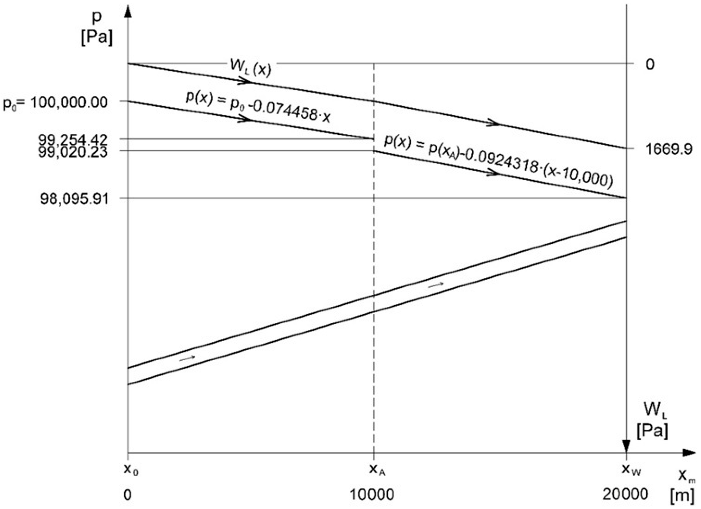
4. Distribution of Static Pressure and Mechanical Energy Losses on the Resistance of Motion in the Duct

The profile research of gas static pressure along its flow in the duct is often used to verify the results of theoretical calculations with the pressure measurements. The models of gas flow in the duct with a point source of heavier gas supply, constant mass flow, and zero momentum were evaluated for the sucking and blowing ventilation systems. The obtained dependences allow for a numerical calculation of the mass flow m ˙ 0 , m ˙ w , mechanical energy losses W L , and finally transport efficiency co-efficient e f , which was the aim of this article. Numerical calculations used the results of article [7], in which the authors determined the same numerical quantities, but for the example of a point source of gas with the same density, source location, mass efficiency, momentum, fan, and duct. For the calculations in article {7} a fan used in underground mines was chosen; its round duct had a large cross-sectional area F = 50 m2, which corresponded to an internal diameter d = 7.98 m. Developed turbulent flow was assumed and its resistance value R*(ρ) = 0.0165 (kg·m)−1 was pointed. In this condition, the point of fan work was calculated and it guaranteed the stable fan operation in the recommended area of its characteristic. To determine the effects of pressure profile p(x) and mechanical energy losses on the resistance of motion W L ( x ) as a function of the current coordinate “x” of the duct, the duct length L should be determined by using the duct parameters from the article in [7]. The following dependencies have to be used:
R ( ρ ) = R ρ 2 = λ L P ρ 8   F 3 ρ 2 = λ L π d 8   F 3 ρ
where P—circumference of the duct cross-section m, from the formula: P =   π d .
Dependency for the tested duct is:
λ L = R ( ρ )   8   F 3 ρ π d = 0.0165 × 8 × 50 3 × 1.2 3.14 × 7.98 = 789.791   m
Assuming the dimensionless distributed resistance coefficient λ = 0.03949 , the calculated duct length is: L = 20,000 m.
The designed duct length indicates that the calculated example will be difficult to verify with measurements; therefore, in order to validate the model, it is better to choose a duct and fan case that will make the validation process easier. The numerical calculation should be done one more time in case of gas inflow with the same density, as in the article [7], and gas inflow with different density, as in the article [7]. It is necessary to construct profiles for all studied locations of gas inflow sources and for several gas mass flow streams with different densities (larger or smaller than ρ = 1.2 kg/m3). Additionally, inflows with different momentum values can be taken into account. Therefore, extensive research and designated profiles of the effects of pressure and mechanical energy losses on the resistance of motion can be easier to use when comparing the results to those of other authors. Mentioned profiles will be presented by the authors in the future, while the procedure of pressure and mechanical energy loss profiles are presented for the duct, which is located in the middle of the duct length ( x a = 10000   m ), local source of mass gas inflow with density ρ = 1.6 kg/m3, and mass stream D ˙ = 50 kg/s.
1 ρ s r F 2 [ 2 m ˙ 0 D ˙ ( x a ) + D ˙ 2 2 ( x a ) ] + p ( x ) p ( x 0 ) + g ( ρ d ρ ) D ˙ ( x a ) m ˙ 0 + D ˙ ( z ( x w ) z ( x a ) ) + R ( x 0 x a ) ( ρ ) · m ˙ 0 2 + R ( x a x w ) ( ρ ) · ( ρ ρ s r ) 2 · ( m ˙ 0 + D ˙ ) 2 = Δ p c ( ρ ) ( ρ s r ρ ) ( x w )
Applying the above equation for the appropriate sections of the duct, it can be written that:
  • For section < x 0 x a > of duct:
    p ( x ) = p ( x 0 ) R ( x 0 x a ) ( ρ ) · m ˙ 0 2 = p ( x 0 ) r ( ρ ) ( x a x 0 ) · m ˙ 0   2 · ( x x 0 )
Because x 0 = 0 , then the dependence on the pressure profile for this section has the form of a decreasing linear function:
p ( x ) = p ( x 0 ) r ( ρ ) ( x a x 0 ) · m ˙ 0   2 · x
For this section of the duct, the mechanical energy losses on the resistance of motion is:
W L ( x ) = r ( ρ ) ( x a x 0 ) · m ˙ 0   2 · x
i.e., an increasing linear function.
At the end of the section, in the point x a , from the side of the point x 0 , the value of preassure and mechanical energy loss is equal:
p ( x a ) = p ( x 0 ) r ( ρ ) ( x a x 0 ) · m ˙ 0   2 · x a
W L ( x a ) = r ( ρ ) ( x a x 0 ) · m ˙ 0   2 · x a
  • For section < x a x w > of the duct, the dependence on the pressure profile is also the decreasing linear function:
    p ( x ) = p ( x a + ) r ( ρ ) ( x a x w ) · ( ρ ρ s r ) 2 · ( m ˙ 0 + D ˙ ) 2 · ( x x a )
At the beginning of the second section, i.e., for x = x a , from the side of the end point x w , the value of pressure is indicate from the equation:
p ( x a + ) = p ( x a ) ( 1 ρ s r F 2 [ 2 m ˙ 0 D ˙ ( x a ) + D ˙ 2 2 ( x a ) ] + g ( ρ d ρ ) D ˙ ( x a ) m ˙ 0 + D ˙ ( z ( x w ) z ( x a ) )   )
For the second section of profile, the mechanical energy losses on the resistance of motion is equal:
W L ( x ) = W L ( x a ) + r ( ρ ) ( x a x 0 ) · ( ρ ρ s r ) 2 · ( m ˙ 0 + D ˙ ) 2 · ( x x a )
It is a linearly increasing function indicating the method of gas flow in the duct.
Inserting the values for profiles of pressure and mechanical energy losses to the equation, the curves presented in the Figure 6, are obtained.

5. Conclusions

Our study of local gas mass sources involving gas with a momentum of zero and density higher than the density of the gas flowing through the duct due to a working fan has led to the following conclusions:
  • If there is a local source of gas mass with a density of 1.6 kg/m3 entering a duct containing gas flowing at a rate of 1.2 kg/m3, the pressure increases in the fan are also loaded by the energy spent to provide the required kinetic energy to this gas mixture with the resultant density.
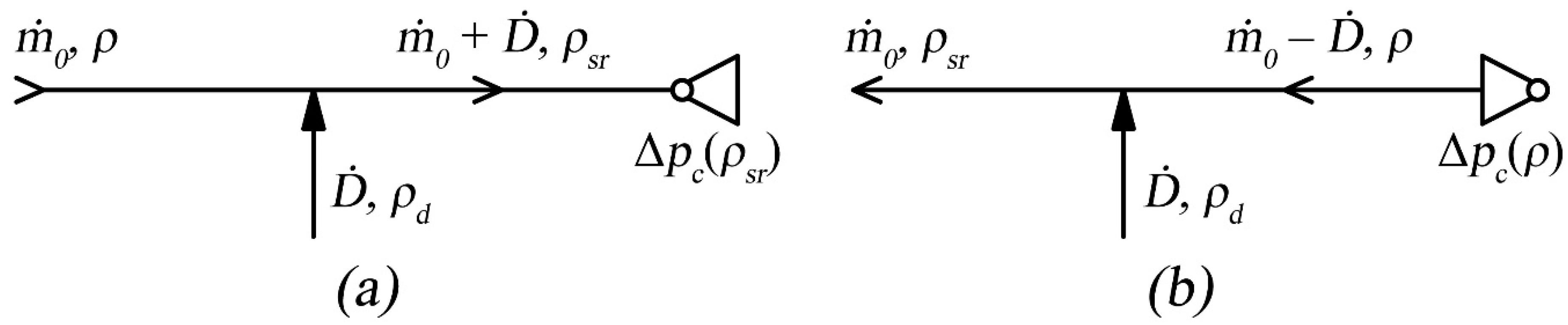
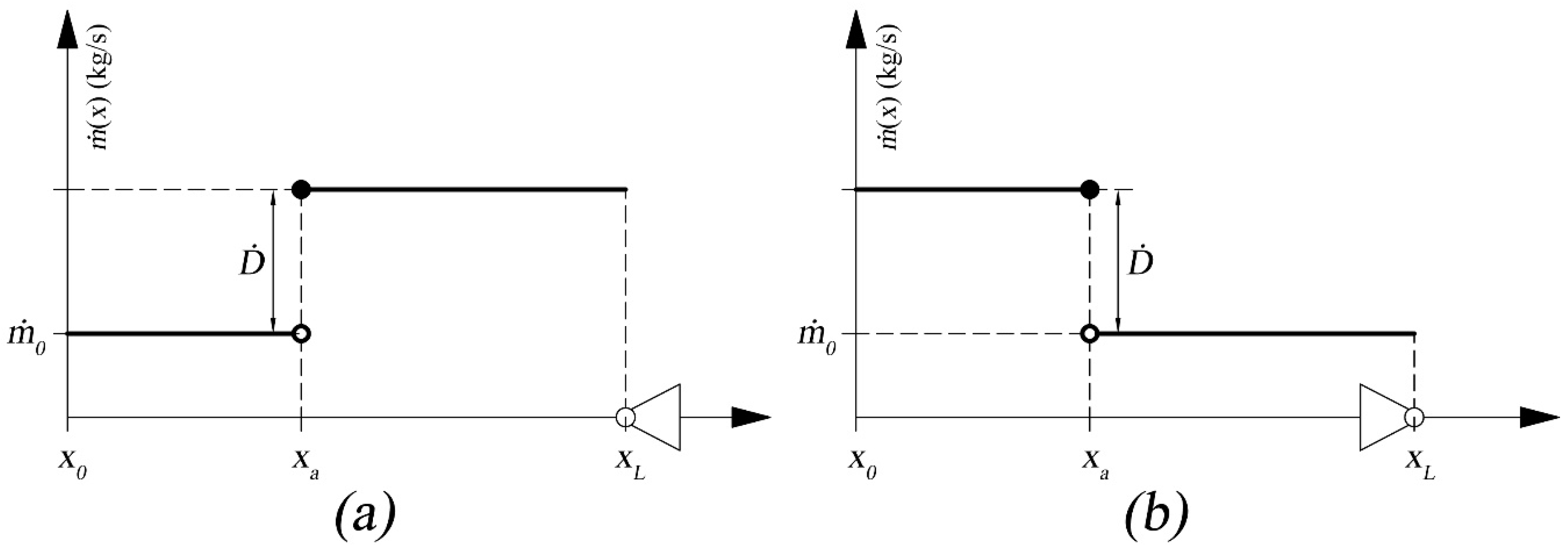
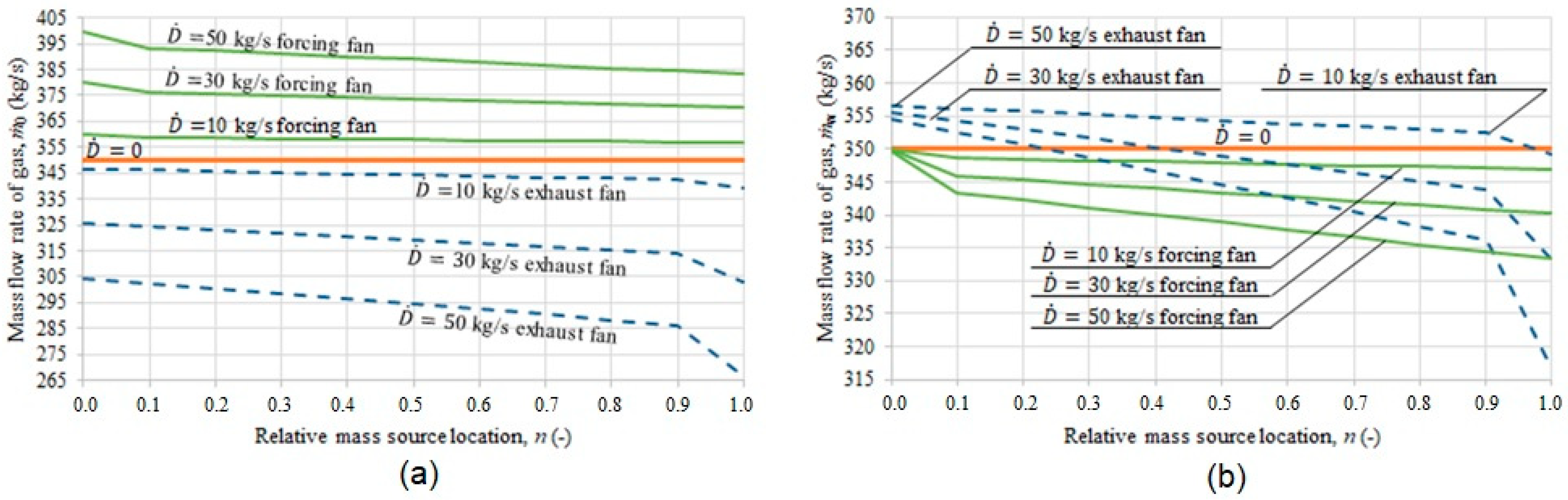
  • If there is a source of gas mass with a different (higher) density, the different duct sections will be passed through by gas with varying density (steady within a range) (Figure 3). If the duct fan is working in the suction mode, the fan will be passed through by gas with an average density of more than 1.2 kg/m3.
  • If the duct fan is working in the blowing mode, gas with a density of 1.2 kg/m3 will be flowing through the fan, regardless of where the local source of gas with a higher density is situated.
  • Changes in the density of gas flowing through the fan require the recalculation of the fan characteristic curve from the catalogue density of 1.2 kg/m3. This means that if the fan is working in the suction mode, the local inflow of gas with varying densities causes changes in the parameters of the mechanical energy source (no such changes occur when the duct fan is working in the blowing mode).
  • Differences in gas densities in different duct sections do not change the relationship between the losses of mechanical energy due to forces of opposing motion. However, these differences do affect the values of these relationships by making it necessary to recalculate the drag values for these duct sections, as shown in Formulas (35) and (36). An increase in density of gas flowing through the duct causes a reduction in the duct’s existing drag.
  • Such differences in gas density between duct sections due to the presence of local sources of gas with varying densities generate mechanical energy in the inclined parts of the duct through which average-density gas is flowing. This energy is associated with a change in the existing buoyancy in this section. This value is defined as natural head and is included for the suction mode of the fan in Formula (29). The local natural head can be negative or positive, depending on the height difference of a duct in which an average-density gas mixture is flowing. This value may differ between duct sections, due to an exhaust or forcing fan. For the same local source of gas mass with a steady flow density, the local natural head for the suction mode is slightly lower than for the blowing mode, as follows from Formulas (31), (32), (37) and (38) for ∆z = 0. The source of gas mass is located at the end of the duct, with the fan working in the suction mode, and conversely, if the source is located at the entry of the duct, with the fan working in the blowing mode, the local natural head is equal to zero.
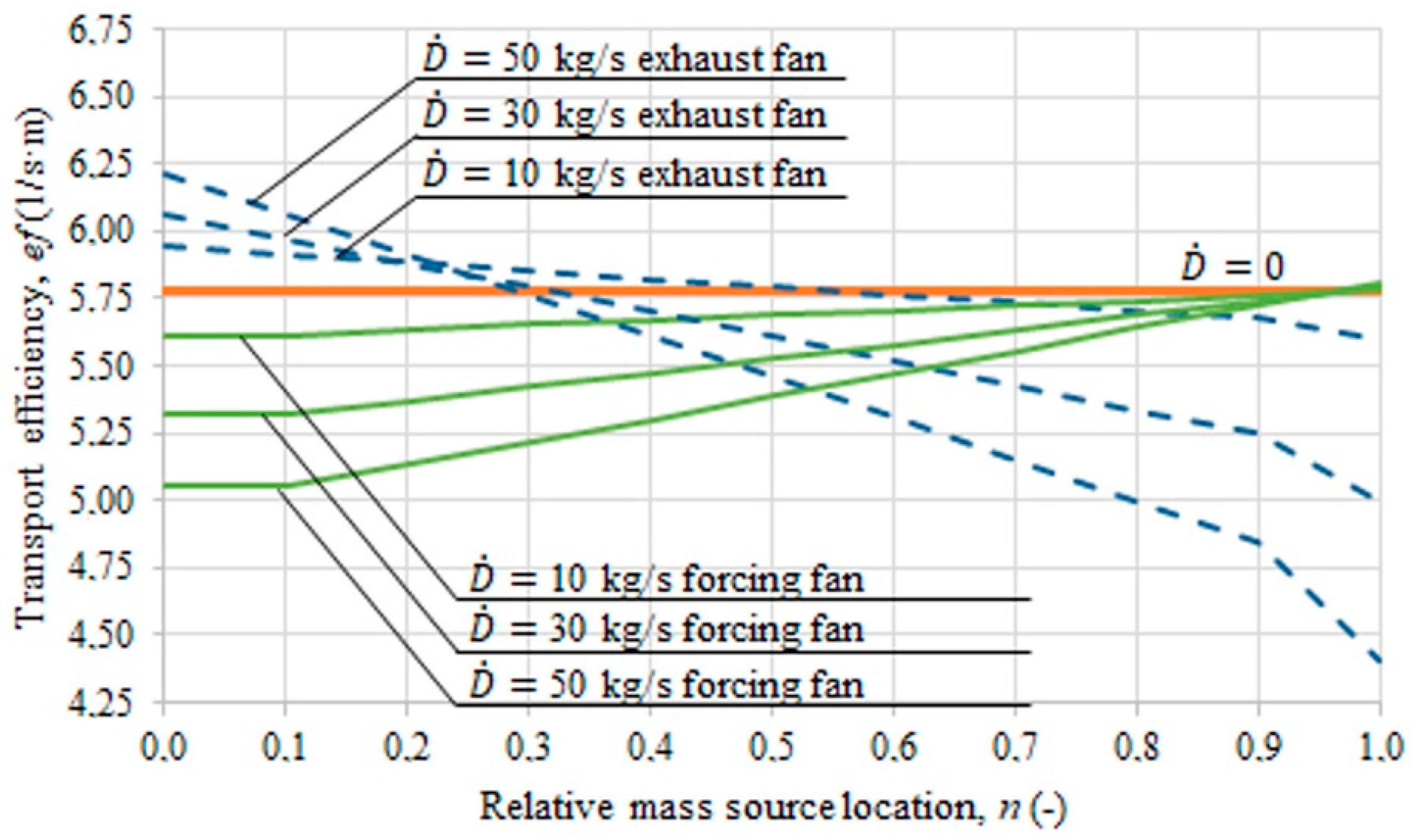
  • The gas transport efficiency is higher with the suction mode of the fan if the gas source of higher density is located closer to the beginning of the duct. Gas transport with greater efficiency requires a greater expenditure of mechanical energy of the fan.
  • The presented mathematical model allows for the determination of the static pressure distribution and mechanical energy loss in the conduit.

Author Contributions

Conceptualization, B.P. and Z.K.; methodology, B.P. and Z.K.; software, B.P. and R.Ł.; validation, Z.K., R.Ł. and P.Ż.; formal analysis, P.Ż. and R.Ł.; investigation, B.P. and Z.K.; resources, B.P.; data curation, R.Ł. and P.Ż.; writing—original draft preparation, Z.K.; writing—review and editing, B.P.; visualization, R.Ł. and P.Ż.; supervision, Z.K.; project administration, Z.K.; funding acquisition, B.P. All authors have read and agreed to the published version of the manuscript.

Funding

The article was supported by the program “Excellence Initiative—Research University” for the AGH University of Science and Technology.

Institutional Review Board Statement

Not applicable.

Informed Consent Statement

Not applicable.

Data Availability Statement

The results of the analysis are presented in the article.

Conflicts of Interest

The authors declare no conflict of interest.

Nomenclature

SymbolParameter
dhydraulic diameter of the duct, m
D ˙ mass efficiency of the gas source (steady value), kg/s
efenergy efficiency for the observed medium’s flow, (m·s)−1
Fcross-sectional area of the duct, m2
g gravity, m/s2
m ˙ mass flow rate of gas, kg/s
m ˙ 0 mass flow rate of gas entering the duct, the opposite end of which features a mechanical suction source (mass flow rate of gas leaving the duct, the opposite end of which features a mechanical a suction source), kg/s
m ˙ w mass flow rate of gas flowing through the fan, kg/s
pabsolute static pressure, Pa
Rspecific drag, Ns2/m8 or kg/m7
R*specific drag of the duct, 1/(kg·m)
r Z A S duct equivalent drag per unit, kg/m8
r Z A S duct equivalent drag per unit, 1/(kg·m2)
W L loss of mechanical energy (total head), N/m2
xcurrent coordinate measured along the duct’s axis, m
zaspot heights at a point of the current coordinates xa, m
zwspot heights at a point of the current coordinates xw, m
δ(xxa), δ(xxw)Dirac delta function distribution, 1/m
δ(xxL)Dirac delta function distribution at the point of local resistance xL, 1/m
Δpc(ρ)fan’s pressure increase when gas with the density ρ is flowing through the fan, Pa
Δpc(ρw)fan’s total pressure increase with the fan flow rate of gas with density ρ, ρ(x) = ρ(xw), Pa
λdimensionless coefficient of distributed resistance, -
ξdimensionless coefficient of local resistance, -
ρddensity of local-source gas stream, kg/m3
ρ(x)gas density at a point with the current coordinate x, kg/m3

References

  1. Bergander, M.J. Fluid Mechanics Vol. 1. Basic Principles; AGH University of Science and Technology Press: Krakow, Poland, 2010. [Google Scholar]
  2. McPherson, M.J. Subsurface Ventilation and Environmental Engineering; Chapman & Hall: London, UK, 1992. [Google Scholar]
  3. Pawiński, J.; Roszkowski, J.; Strzemiński, J. Przewietrzanie Kopalń; Śląskie Wydawnictwo Techniczne: Katowice, Poland, 1995. [Google Scholar]
  4. Wacławik, J. Mechanika Płynów i Termodynamika; Wydawnictwo AGH: Krakow, Poland, 1993. [Google Scholar]
  5. Yamaguchi, H. Engineering Fluid Mechanics; Springer: Cham, The Netherlands, 2010. [Google Scholar]
  6. Ptaszyński, B. Charakterystyka przepływowa przewodu transportującego różne media. In Proceedings of the 8 Szkoła Aerologii Górniczej. Sekcja Aerologii Górniczej: Nowoczesne Metody Zwalczania Zagrożeń Aerologicznych w Podziemnych Wyrobiskach Górniczych, Jaworze, Poland, 13–16 October 2015; Dziurzyński, W., Ed.; Główny Instytut Górnictwa: Katowice, Poland, 2015. [Google Scholar]
  7. Ptaszyński, B.; Łuczak, R.; Życzkowski, P.; Kuczera, Z. Transport Efficiency of a Homogeneous Gaseous Substance in the Presence of Positive and Negative Gaseous Sources of Mass and Momentum. Energies 2022. in print. [Google Scholar]
  8. Wacławik, J. Wentylacja Kopalń, Tom I, II; Wydawnictwo AGH: Krakow, Poland, 2010. [Google Scholar]
  9. Bunko, T.; Shyshov, M.; Myroshnychenko, V.; Kokoulin, I.; Dudnyk, M. Estimation and use materials of the airily-depressed surveys on the coal mines of Ukraine. International Conference Essays of Mining Science and Practice. E3S Web Conf. 2019, 109, 13. [Google Scholar] [CrossRef]
  10. Zmrhal, V.; Boháč, J. Pressure loss of flexible ventilation ducts for residential ventilation: Absolute roughness and compression effect. J. Build. Eng. 2021, 44, 103320, ISSN 2352-7102. [Google Scholar] [CrossRef]
  11. Dziurzyński, W.; Krach, A.; Pałka, T. Airflow Sensitivity Assessment Based on Underground Mine Ventilation Systems Modeling. Energies 2017, 10, 1451. [Google Scholar] [CrossRef]
  12. Szmuk, A.; Kuczera, Z.; Badylak, A.; Cheng, J.; Borowski, M. Regulation and control of ventilation in underground workings with the use of VentSim software. In Proceedings of the International Conference on Energy, Resources, Environment and Sustainable Development, Xuzhou, China, 26–27 May 2022; p. 102. [Google Scholar]
  13. Dziurzyński, W.; Krawczyk, J. Możliwości obliczeniowe wybranych programów symulacyjnych stosowanych w górnictwie światowym, opisujących przepływ powietrza, gazów pożarowych i metanu w sieci wyrobisk kopalni. Przegląd Górniczy Miesięcznik Stowarzyszenia Inżynierów Tech. Górnictwa 2012, 68, 1–11. [Google Scholar]
  14. Semin, M.A.; Levin, L.Y. Stability of air flows in mine ventilation networks. Process Saf. Environ. Prot. 2019, 124, 167–171. [Google Scholar] [CrossRef]
  15. Onder, M.; Cevik, E. Statistical model for the volume rate reaching the end of ventilation duct. Tunn. Undergr. Space Technol. 2008, 23, 179–184. [Google Scholar] [CrossRef]
  16. Auld, G. An estimation of fan performance for leaky ventilation ducts. Tunn. Undergr. Space Technol. 2004, 19, 539–549. [Google Scholar] [CrossRef]
  17. Jiang, H.; Lu, L.; Sun, K. Experimental study and numerical investigation of particle penetration and deposition in 90 bent ventilation ducts. Build. Environ. 2011, 46, 2195–2202. [Google Scholar] [CrossRef]
  18. Sleiti, A.K.; Zhai, J.; Idem, S. Computational Fluid Dynamics to Predict Duct Fitting Losses: Challenges and Opportunities. HVAC&R Res. 2013, 19, 2–9. [Google Scholar] [CrossRef]
  19. Akhtar, S.; Kumral, M.; Sasmito, A.P. Correlating variability of the leakage characteristics with the hydraulic performance of an auxiliary ventilation system. Build. Environ. 2017, 121, 200–214. [Google Scholar] [CrossRef]
  20. Sharma, S.K.; Kalamkar, V.R. Computational Fluid Dynamics approach in thermo-hydraulic analysis of flow in ducts with rib roughened walls—A review. Renew. Sustain. Energy Rev. 2016, 55, 756–788. [Google Scholar] [CrossRef]
  21. Yu, H.; Xu, H.; Fan, J.; Zhu, Y.; Wang, F.; Wu, H. Transport of Shale Gas in Microporous/Nanoporous Media: Molecular to Pore-Scale Simulations. Energy Fuels 2021, 35, 911–943. [Google Scholar] [CrossRef]
Figure 1. Gas flow chart for Example 1 under consideration of a (a) fan working in the suction mode, (b) fan working in the blowing mode.
Energies 15 05834 g001
Figure 2. Plot of the function m ˙ ( x ) for Example 1: (a) fan working in the suction mode, (b) fan working in the blowing mode.
Energies 15 05834 g002
Figure 3. Plot of the function ρ(x) for Example 1: (a) fan working in the suction mode, (b) fan working in the blowing mode.
Energies 15 05834 g003
Figure 4. Results of numerical calculations for analyzing examples: (a)—mass flow rate of gas entering the duct m ˙ 0 , (b)—mass flow rate of gas flowing through the fan m ˙ w .
Energies 15 05834 g004
Figure 5. Duct gas transport efficiency in the presence of a local source of gas with different densities for examples 1a and 1b.
Energies 15 05834 g005
Figure 6. The profile of pressure and mechanical energy loss in the duct for the case of mass gas inflow with zero momentum.
Energies 15 05834 g006
Publisher’s Note: MDPI stays neutral with regard to jurisdictional claims in published maps and institutional affiliations.

