An Accurate Power Flow Method for Microgrids with Conventional Droop Control

Abstract

With conventional droop control, the droop relationship between the voltage and reactive power is not purely linear because of the filter reactance. This paper focuses on the theoretical analysis to account for this characteristic and presents a precise power flow method for conventional droop control. The proposed method is universal, which can handle not only conventional droop control, but also other control strategies, such as robust droop control, constant power control, and constant voltage–frequency control. It can also handle frequency-dependent active and reactive power loads and is adapted for islanded and grid-connected systems. The proposed method extends the applicability of conventional power flow methods to microgrids so that the framework of the method is generic; any conventional power flow algorithm can be adapted to this framework. Compared with the time-domain simulation method, the proposed method is accurate, simple, and easy to implement for industrial applications.

1. Introduction

Small autonomous regional power systems can offer increased reliability and efficiency and can aid in the integration of renewable energy and other forms of distributed generation (DG) [1,2]. Many forms of DG such as fuel cells, photovoltaic systems, and micro turbines are interfaced with the network through power electronic inverters [3]. These interface devices make the sources more flexible in operation and control when compared with conventional electrical machines. The inverter includes four parts: voltage conversion, power electronic switching devices, LC/LCL filter circuits, and control strategy. Currently, the main control strategy is to simulate the external characteristics of the traditional synchronous generator. In the early stages, a proportional–integral (PI) controller was used to put the inverter into constant PQ/PV/Vf mode. In recent years, to adapt to the more complex operating environment of a microgrid, several control strategies have emerged that can participate in the management of the system frequency and voltage regulation. These include conventional droop control, robust droop control, the virtual synchronous generator (VSG), and various improved control algorithms, shown in Table 1. Research in the field of inverters has significantly promoted the development of microgrids.

Table 1. Control strategies of inverters and characteristics.

Number	Control Strategies	Characteristic
I	Constant $PQ$ control	Both the P and Q units contain integrators; $\omega ,\delta ,v_r$ are generated separately; P and Q are maintained constant
II	Constant $Vf$ control	Both the V and f units contain integrators, and V and f are maintained constant
III	Constant $PV$ control	Both the P and V units contain integrators, and V and f are maintained constant
IV	Robust droop control	Both the $P-\omega$ and $Q-V$ units contain integrators, which improves the average power distribution
V	Conventional droop control	Only the $P-\omega$ unit contains integrators

Power flow studies are essential for the planning and design of future power system expansion. In addition, power flow studies play an important role in state analysis, stability evaluation, and optimal management [4]. In the microgrid, power flow calculation is related to the control strategies of inverters. The DGs need to be equivalent to a node type that matches the inverter control strategy.

In Table 1, when inverters adopt control strategy I–III, DGs are equivalent to the PQ, Vf, and PV node types of traditional power flow calculation. It is the same as the traditional power flow calculation both in modeling and algorithm.

When inverters adopt control strategy $IV$, that is robust droop control [5], DGs cannot be made equivalent to conventional node types because, as a result of robust droop control, the active and reactive power output depend on the terminal voltage and system frequency. Thus, conventional power flow methods cannot be applied to an islanded microgrid [6,7]. In robust droop control, both $\mathcal{P}-\omega$ and $\mathcal{Q}-\mathcal{V}$ droop are linear. Several new methods have been studied to solve the power flow problem for robust droop control. Reference [8] developed a three-phase power flow algorithm for islanded microgrids, in which some DG units are controlled by their droop characteristics. The problem is formulated as a set of nonlinear equations, and a Newton trust region method is used to solve the power flow problem. In [9], the droop relationships between the voltage and reactive power are included in the load flow equations, and particle swarm optimization is used to analyze the power flow. The proposed schemes are accurate, but complex. In [10], the Newton–Raphson (NR) algorithms are combined with the droop characteristic of the DG to solve the power flow problem. In [11], a universal power flow algorithm is proposed to handle the active control strategies of the DGs, including isochronous control, droop control, and constant power control. In [12], an iterative procedure based on a mathematical formulation of conventional power flow is introduced to calculate the equilibrium operating point in the islanded microgrids, and the slack bus voltage is determined through a binary search method, which may increase the number of iterations in some cases. In [13], by considering the virtual impedance in the microgrid, the proposed methods obtain more accurate calculation results for the power flow analyses. In [14], an advanced Newton approach is developed to assess power sharing and voltage regulation. It incorporates droop control and various secondary control modes into a modified Jacobian matrix, so convergence relies on the selection of good initial values.

The backward/forward sweep (BFS) algorithm has been proven to be fast and efficient for both radial and weakly meshed distribution networks, because of the absence of the complex Jacobian matrix and its inverse [15]. Reference [16] proposes a method based on a BFS algorithm to solve the power flow problem in AC droop-regulated microgrids, and this represents the first derivative-free algorithm to solve droop control power flows in islanded microgrids. However, the reactive powers supplied by the DGs are only dependent on their droop coefficient, and local voltages are ignored. A modified BFS algorithm is presented in [17], in which the DG reactive powers are made to rely not only on their droop coefficients, but also on local voltages; however, conflicting updates issued by the voltage give convergence problems.

When inverters adopt control strategy V, that is the conventional droop control [18], considering the effects of the filter reactance, $\mathcal{Q}-\mathcal{V}$ is not a simple linear droop relationship that is determined by the droop parameters, reactance parameters, and operating state. If the filter reactance is ignored, the above literature [8,9,10,11,12,13,14,15,16,17] for robust droop control is also suitable for conventional droop control. However, in low-voltage microgrids, the filter reactance is many times higher than the circuit reactance and, so, cannot be ignored. The details of why reactance cannot be ignored are given in Appendix A. Therefore, as a result, the existing methods cannot accurately calculate the power flow solution under the conventional droop control scheme.

In addition, it usually contains DGs of different control strategies in the microgrid; the power flow calculation model should be universal, which is applicable to various types of control strategies. However, the existing methods are mainly aimed at robust droop control [9,10,12,13,14,16,17]. Reference [11] is able to be applied to all kinds of control strategies, but only focused on frequency-active power control of DGs.

Thirdly, the existing algorithms mainly make modifications to the specified conventional power flow method [8,9,10,11,13,14,16,17], so that the algorithm framework is not generic. In order to facilitate industrial application, the algorithm should be generic, that is it is not limited to a specified conventional power flow calculation method.

To overcome the aforementioned problems, this paper proposes a method to analyze the power flow for microgrids. Its main contributions are as follows:

1.

The paper describes a new power flow method, which is able to deliver accurate results for conventional droop control in low-voltage microgrids, e.g., the marine microgrid. The method takes into account the filter reactance, which cannot be ignored in the low-voltage grid. With modeling the filter reactance in the power flow formulation, the calculation accuracy is improved compared with those using traditional methods.

2.

The proposed algorithm is universal for power flow in microgrids. It can handle islanded and grid-connected systems and can adapt to various DG control strategies, including conventional droop control, robust droop control, constant power control, and constant Vf control. It also can handle frequency-dependent active and reactive loads.

3.

The framework of a general power flow method for the microgrid is presented to reduce the difficulty and the complexity of program development. The proposed algorithm takes the conventional power flow algorithm and expands it to adapt to the droop characteristics through two iterative loops; it is easy to implement.

The comparison between the proposed method and several existing approaches is shown in Table 2.

Table 2. Comparison between power flow approaches.

	MNR Method [10]	Ref. [11]	Ref. [12]	Ref. [13]	DBFS Method [16]	Proposed Method
Different control strategies	No	Yes	No	No	No	Yes
Generic algorithm framework	No	No	No	No	No	Yes
Considering filter reactance	No	No	No	No	No	Yes
Various network configuration of microgrids	Yes	Yes	Yes	Yes	No	Yes
Grid-connected	No	Yes	no	No	No	Yes
Islanded	Yes	Yes	Yes	Yes	Yes	Yes

2. Control Strategy of Conventional Droop Control

2.1. Structure of Inverter in Microgrids

Figure 1 shows an inverter connected to a microgrid bus that includes a power electronics unit, LC filter unit, control unit, and line impedance unit [19], where ${\mathbf{V}}_c$ is the capacitor voltage, $i_L$ is the inductance current on the inverter side, $Z_{line}$ is the line impedance, and ${\nu }_r$ is the pulse width modulation signal of the inverter. The frequency, voltage amplitude, output power, and other information are obtained by measuring ${\mathbf{V}}_c$ and $i_L$, and modulated waves ${\nu }_r$ are generated by various control strategies to finish the power control.

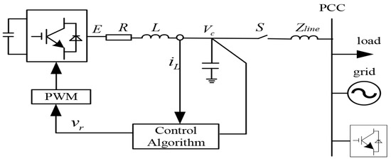
Figure 1. Inverter structure of microgrids.

2.2. Conventional Droop Control

Droop control is a control strategy that simulates the external characteristics of a synchronous generator set, in which frequency and voltage are regulated by the relationship between frequency and active power and voltage and reactive power. Since droop control was proposed, many ways to implement it have been available. Figure 2 shows a conventional droop control block [20]. Reactive-voltage droop control does not contain integrators, and the following equations represent the droop operation of the inverter.

$$E_i=E^{*}-n_i({\mathcal{Q}}_i-{\mathcal{Q}}_{ref,i})$$

(1)

$${\omega }_i={\omega }^{*}-m_i({\mathcal{P}}_i-{\mathcal{P}}_{ref,i})$$

(2)

where $E^{*}$ and ${\omega }^{*}$ are the voltage reference value and angular frequency reference value, respectively, ${\mathcal{P}}_i$ and ${\mathcal{Q}}_i$ are the active and reactive powers generated by the DG, respectively, ${\mathcal{P}}_{ref,i}$ and ${\mathcal{Q}}_{ref,i}$ are the active and reactive power reference value, respectively, and $m_i$ and $n_i$ are the frequency and voltage droop coefficients, respectively.

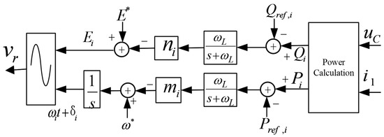
Figure 2. Conventional droop control.

Figure 2 shows that the modulation wave ${\nu }_r$ is controlled based on a linear droop relationship to participate in the system’s voltage and frequency modulation. However, Figure 1 shows that an LC filter is at the inverter outlet. Because the reactance of the filter is much higher than the reactance of the line in the low-voltage microgrid system, the effect of the filter reactance on the power flow cannot be ignored. The steady state is shown in Figure 3.

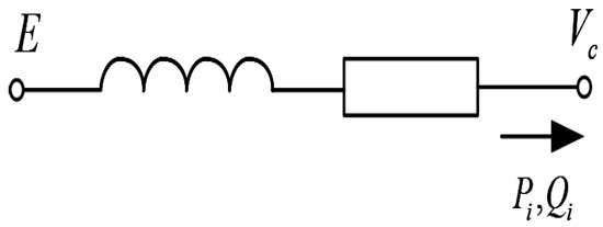
Figure 3. Filter structure.

The reactive power output by the inverter is:

$$Q_i=\frac{V_c\left[X_L(E_{i}cos\delta -V_c)-E_{i}Rsin\delta \right]}{R^2+X_L^2}$$

(3)

Considering that the resistance R of the filter is very low, it can be ignored, and because the phase angle difference between the two ends of the reactance is small, it can be assumed to be zero. From (1) and (3), the voltage $V_c$ can be expressed as [21]:

$$V_c=\frac{E^{*}-n_i(Q_i-Q_{ref,i})}{2}-\frac{\sqrt{{[n_i(Q_i-Q_{ref,i})-E^{*}]}^2-4(Q_i-Q_{ref,i})X_L}}{2}$$

(4)

The derivation of the voltage to reactive power is

$$\frac{d{V}_c}{d{Q}_i}=-\frac{n_i}{2}-\frac{n_i[n_i(Q_i-Q_{ref,i})-E^{*}]-2X_L}{2\sqrt{{[n_i(Q_i-Q_{ref,i})-E^{*}]}^2-4(Q_i-Q_{ref,i})X_L}}$$

(5)

From (5), the terminal voltage $V_c$ and reactive power $Q_i$ do not have a simple linear droop relationship, because they are affected by the filter reactance $X_L$. If $X_L=0$, then $\frac{d{V}_c}{d{Q}_i}=-n_i$.

3. The Proposed Method

To reduce the difficulty of program development, this paper extends the conventional power flow calculation method to solve new problems. Reference [16] iteratively updates the frequency and voltage through two nested loops to reflect the robust droop control characteristics, which is easy to implement. This paper also adopted this idea; the difference is that the filter is taken into account in conventional droop control and the method framework is universal.

The proposed algorithm includes four parts: setting the initial conditions, conventional power flow calculation, frequency update, and bus voltage update with filter reactance.

3.1. Initial Conditions’ Setting

First, the virtual slack bus, which can be selected randomly in microgrid buses, should be selected to emulate the upstream utility grid. The iterative procedures adjust the voltage of the virtual slack bus and grid frequency to show the islanded operation of the DG. The frequency f was initialized to its nominal value. The active power $P_i$ and reactive power $Q_i$ of the DG were initialized to their reference values $P_{ref.i}$ and $Q_{ref,i}$, and all the bus voltages were set to 1.0. As a variety of control strategies of inverters may be contained in a microgrid, the droop coefficients and filter reactance depend on the control strategies of the inverter. For conventional droop control, the droop coefficients $m,n$ and filter reactance $X_L$ were set to given values. For robust droop control, $X_L$ was set to zero. For constant power control, m and n were set to zeros.

3.2. Conventional Power Flow Calculation

The framework of the algorithm is generic, not limited to a specified conventional power flow method. The BFS method, the NR method, and others are all applicable. Owing to the radial structure of most microgrids and the simple calculation involved in the BFS method, a matrix-based BFS was adopted in this paper. The basic steps are as follow [22]:

Step 1: Calculate the bus injection current $I_{bus}$:

$$I_{bus}^i={\left(\frac{P_i-P_{Li}+Q_i-Q_{Li}}{V_i}\right)}^{*}$$

(6)

where $P_{Li}$ and $Q_{Li}$ are the load power, which are frequency-dependent and can be expressed as follows

$$P_{Li}=(c_{1i}{f}_{pu}^2+c_{2i}{f}_{pu}+c_{3i})P_{Li.N}$$

(7)

$$Q_{Li}=(d_{1i}{f}_{pu}^2+d_{2i}{f}_{pu}+d_{3i})Q_{Li.N}$$

(8)

Step 2: Calculate the branch current $I_{branch}$:

$$I_{branch}=BIBC·I_{bus}$$

(9)

where $BIBC$ is the transformation matrix from the bus injection current to the branch current containing the elements 0 and 1. For a radial system of n buses, the $BIBC$ matrix is an upper triangular matrix with dimensions $n-1\times n-1$.

Step 3: Calculate the bus voltage:

$$V_{bus}=V_{sb}-BCBV·I_{branch}$$

(10)

where $V_{sb}$ is the slack bus voltage. The $BCBV$ matrix is the transformation matrix to calculate the voltage difference between the slack bus and other buses from the branch currents. The elements of $BCBV$ are impedances. Given a system of n buses, the resulting $BCBV$ matrix will be of dimensions $n-1\times n-1$. Refer to [23] for the specific process. The power carried by the virtual slack bus is calculated after the convergence of the BFS method.

$$P_{sb}+j{Q}_{sb}=V_{sb}·\sum {I_{sb}}^{*}-(P_{Gsb}+j{Q}_{Gsb})+(P_{Lsb}+j{Q}_{Lsb})$$

(11)

where $\sum I_{sb}$ represents all the branch currents connected to the slack bus, $P_{Gsb}+j{Q}_{Gsb}$ is the virtual slack bus generation power (if the virtual slack bus is not a DG bus, $P_{Gsb}+j{Q}_{Gsb}=0$), and $P_{Lsb}+j{Q}_{Lsb}$ is the virtual slack bus load power.

3.3. Frequency Update

If $\left|P_{sb}\right|>\epsilon$ ($\epsilon$ is the predefined tolerance), $P_{sb}$ will be allocated to all DG units to make the virtual slack bus carry zero power. The mathematical expression is given by (12), while according to the droop characteristic, the power allocated to each DG satisfies (13).

$$\sum _{i=1}^{N_g}\mathsf{\Delta }{P}_i=P_{sb}$$

(12)

$$m_1\mathsf{\Delta }{P}_1=\cdots =m_{N_g}\mathsf{\Delta }{P}_{N_g}$$

(13)

$${P_i}^{\left(k\right)}={P_i}^{(k-1)}+\mathsf{\Delta }{P}_i$$

(14)

The power allocated to each DG can be obtained from (12) and (13), and f can be updated from (2). The active power and frequency are updated iteratively until $\left|P_{sb}\right|<\epsilon$. Refer to the frequency update loop in Figure 4 for the specific iterative process.

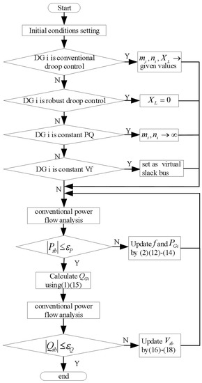
Figure 4. Flowchart of the proposed algorithm.

3.4. Bus Voltage Update Considering Filter

When the frequency update terminates, the voltage is no longer the initial value, and the reactive power of the DG should also change according to the droop characteristic.

The inverter terminal voltage $V_c$ and reactive power Q do not show the linear droop characteristic that is shown between the filter left side voltage E and reactive power Q. E is calculated from the bus voltage V of the DG as follows:

$$E_i=V_i+I_i·j{X}_{Li}$$

(15)

The reactive power of the DG can be calculated by substituting (15) into (1). The power flow is calculated again, and if the reactive power carried by the virtual slack bus $\left|Q_{sb}\right|>\epsilon$, as with the frequency update, it indicates that the voltage solution has not reached the steady state, so $Q_{sb}$ should be allocated to all DG units.

$$\sum _{i=1}^{N_g}\frac{1}{n_i}\mathsf{\Delta }{E}_i=Q_{sb}$$

(16)

Unlike with the frequency, the voltages, $E_i$, at each inverter bus are different. This difference is mainly caused by the line impedance. However, the voltage deviation $\mathsf{\Delta }{E}_i$ is not significant. Therefore, assuming that the voltage deviation for each DG is equal to the voltage deviation at the slack bus, it can be expressed as follows:

$$\mathsf{\Delta }{E}_1=\mathsf{\Delta }{E}_2=\cdots \cdots =\mathsf{\Delta }{E}_{N_g}=\mathsf{\Delta }{V}_{sb}$$

(17)

The voltage deviation $\mathsf{\Delta }{V}_{sb}$ of the slack bus can be approximated by substituting (17) into (16).

The slack bus voltage is updated as:

$${V_{sb}}^{\left(k\right)}={V_{sb}}^{(k-1)}-\mathsf{\Delta }{V}_{sb}$$

(18)

Subsequently, the voltage of the DG is updated by the power flow calculation for the next iteration.

3.5. Processing Flow of the Proposed Method

The specific process of the proposed method is shown in Figure 4, which summarizes the steps in the method.

After the initial parameters are given, the control strategies of the DG and setting corresponding parameters $m,n$, $X_L$ are checked. Next, the conventional power flow calculation is carried out to check whether the active power taken up by the DGs is balanced with the load power. If not, the system frequency is updated according to the DG control characteristics. Finally, the reactive power of the DGs is calculated according to the new voltage, and the power flow calculation is carried out again to check whether the reactive power taken up by the DGs is balanced with the load power. If not, the voltages are updated according to the DGs’ control characteristics. The convergence conditions of frequency update may be violated because frequency updates are not decoupled from voltage updates. For instance, voltage updates lead to changes in power losses in the line, and then, the active power distribution of the network is changed. Therefore, two nested loops of voltage and frequency are adopted to ensure that the frequency and voltage converge.

4. Generalization of the Proposed Method

4.1. Applicability to the Conventional Power Flow Algorithm

As shown in Figure 4, the conventional power flow algorithm is extended and modified through inner and outer loops to reflect the droop characteristic of the DG. The proposed method is not limited to the specific conventional power flow method; therefore, the proposed framework is generic, and any conventional power flow algorithm, including NR, current injection, and other methods, can be adapted to this framework.

4.2. Applicability to the Inverter Control Strategies

Although the algorithm is designed for conventional droop control, it can be applied to other control strategies. The explanation is as follows:

(1) Robust droop control:

When the DG inverters have robust droop control strategies, the inverter terminal voltage $V_c$ and reactive power Q have a linear droop relationship. This characteristic can be expressed by setting reactance $X_L$ to zero in the proposed algorithm. The inverter terminal voltage $V_c$ and reactive power Q have a linear droop relationship.

(2) Constant PQ control:

When the DG inverters have constant PQ control strategies, the frequency and voltage droop coefficients $m_i$ and $n_i$ are set as infinite. The power deviation is:

$$\mathsf{\Delta }{P}_{Gi}=\frac{\mathsf{\Delta }f}{m_i},\mathsf{\Delta }{Q}_{Gi}=\frac{\mathsf{\Delta }E}{n_i}$$

(19)

Then, the deviations in the active power and reactive power are zero, and P and Q are constant.

(3) Constant Vf control:

When the inverter has a constant Vf control strategy, the inverter is connected to the main grid, which acts as the slack bus in the system, while the other DG inverters usually have a constant PQ strategy. In this case, the inverter is selected as the virtual slack bus.

5. Numerical Validation

The 33-bus test system with five DGs shown in Figure 5 was adopted to validate the proposed algorithm [16]. The DG nominal power and droop coefficients are shown in Table 3. In the following scenarios, load coefficients $c_{1i}=d_{1i}=0.2$, $c_{2i}=d_{2i}=0.3$ and $c_{3i}=d_{3i}=0.5$ for all loads. We selected bus 1 randomly to be the virtual slack bus. The power flow results of the proposed method (PM) were compared with those obtained by time-domain simulation (TDS).

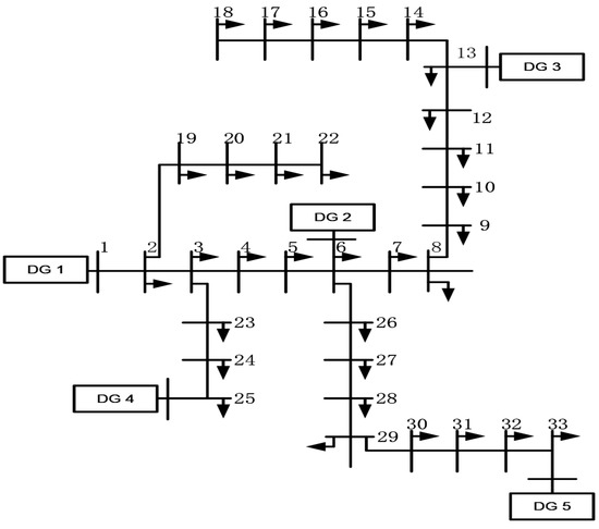
Figure 5. The 33-bus test system under study.

Table 3. Control parameters of DG.

	Pref (pu)	Qref (pu)	Droop Coefficient
			mi	ni
DG1	0.9	0.9	0.05	0.05
DG2	0.9	0.9	1	1
DG3	0.9	0.9	0.1	0.1
DG4	0.9	0.9	1	1
DG5	0.9	0.9	0.2	0.2

5.1. Islanded Grid with Conventional Droop Inverters

In this scenario, all the DG inverters operate in conventional droop mode. The filter reactance for all inverters is $X_L=1.5$ [24,25]. The voltage magnitudes and power of the PM and TDS are listed, respectively, in Table 3 and Table 4, and the tables show that the voltage magnitude and DG power are very close to the acceptable error limits. The results obtained by the PM match the results obtained from the TDS; the system frequency is equal to 0.9297, which is the same as in the TDS. Owing to the proposed algorithm taking into account the influence of reactance by Formulas (15)–(17), the accurate power flow results are obtained.

Table 4. Power and frequency for conventional droop control.

	PM		TDS		MBFS
	P	Q	P	Q	P	Q
DG1	2.3061	0.8524	2.306	0.8523	2.306	0.8533
DG2	0.9703	0.9023	0.97	0.9022	0.9703	0.9026
DG3	1.603	0.8335	1.6034	0.8337	1.603	0.8332
DG4	0.9703	0.9016	0.97	0.9015	0.9703	0.9018
DG5	1.2515	0.9117	1.2511	0.9116	1.2515	0.9133
f	PM		TDS		${\mathit{X}}_{\mathit{L}}$omitted
	0.9297		0.9297		0.9297

Figure 6 and Table 4 also list the results based on the MBFS algorithm [17]. The reactance $X_L$ was ignored in this method. It can be seen that the method of ignoring the reactance converges to the same active power and frequency results with the TDS. However, compared with the TDS, the absolute voltage error maximum was 0.0041 and the relative error maximum was 0.41%, and the reactive power results had errors as well, which indicates that the error was the result of ignoring the reactance. The inherent approximation can result in significant errors depending on the values of reactance $X_L$. The proposed method provides a more accurate approach to solve the power flow for conventional droop.

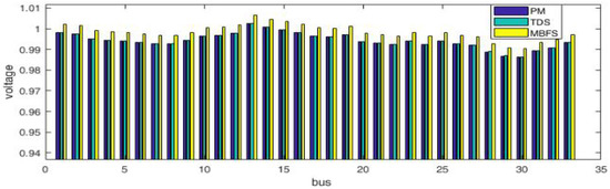
Figure 6. Voltage results for conventional droop control.

5.2. Impact of Filter Reactance $X_L$

In the previous subsection, the method of ignoring the reactance and the proposed method yielded different results. Even though the results were different, the error was small. In this scenario, the load power changes from 50% to 150%, that is the power carried by the DGs gradually increases, and other conditions are the same as 5.1. The relative voltage error maximum of the proposed method and the MBFS method in which the reactance is ignored are shown in Figure 7; it can be seen that the errors caused by ignoring the reactance increase with the increase of the DG power output. This increase in error is due to the increase in filter current. For the method of ignoring the reactance, when the reactive power carried by the DG increases by $\mathsf{\Delta }{Q}_i$, the inverter terminal voltage can be expressed as

$$V_i^{omitted}=E^{*}-n_i\mathsf{\Delta }{Q}_i$$

(20)

The accurate voltage result obtained by the proposed algorithm should be:

$$V_i^{pm}=E^{*}-n_i\mathsf{\Delta }{Q}_i-jI{X}_L$$

(21)

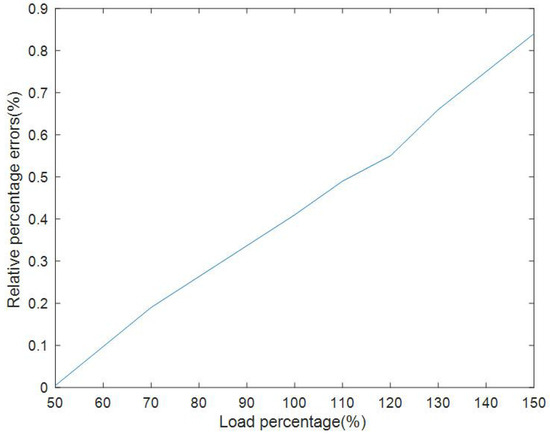
Figure 7. Relationship between voltage error and DG power.

It can be seen from (20) and (21) that, in addition to the reactance value, the voltage error is also proportional to the filter current. When the power carried by the DG increases, the current flowing through the filter increases, then the voltage error increases.

5.3. Islanded Grid with Various Control Strategies

In this scenario, DG1 and DG2 operate in conventional droop mode, DG3 and DG4 operate in robust droop mode, ${X_L}_3={X_L}_4=0$, and DG5 operates in constant PQ mode, $m_5=n_5=\infty$. The other conditions are the same as in 5.1. The results are listed in Table 5, which shows that the results obtained by the proposed method match the results obtained by the TDS. Because DG5 is under constant power control and does not participate in droop sharing, the other four DGs have to carry more load power, and the system frequency is 0.9201, which is reduced compared with Table 4.

Table 5. Power flow results for 5.3 and 5.4.

Bus	Case of 5.3		Case of 5.4
	PM	TDS	PM	TDS
1	1.0002	1.0002	1	1
2	0.9994	0.9994	0.997	0.997
3	0.9966	0.9966	0.9829	0.9829
4	0.9957	0.9957	0.9755	0.9755
5	0.995	0.995	0.9681	0.9681
6	0.9939	0.9939	0.9497	0.9497
7	0.9935	0.9935	0.9462	0.9462
8	0.9937	0.9937	0.9413	0.9413
9	0.9956	0.9956	0.9351	0.9351
10	0.9981	0.9981	0.9292	0.9292
11	0.9986	0.9986	0.9284	0.9284
12	0.9996	0.9996	0.9269	0.9269
13	1.0051	1.0051	0.9208	0.9208
14	1.0036	1.0036	0.9185	0.9185
15	1.0019	1.0019	0.9171	0.9171
16	1.0008	1.0008	0.9157	0.9157
17	0.999	0.999	0.9137	0.9137
18	0.9987	0.9986	0.9133	0.9132
19	0.9989	0.9989	0.9965	0.9965
20	0.9955	0.9955	0.9929	0.9929
21	0.9948	0.9948	0.9922	0.9921
22	0.9942	0.9941	0.9916	0.9916
23	0.9956	0.9956	0.9794	0.9794
24	0.9942	0.9942	0.9727	0.9727
25	0.9959	0.9959	0.9694	0.9694
26	0.9931	0.9931	0.9477	0.9477
27	0.9921	0.9921	0.9452	0.9452
28	0.9877	0.9877	0.9337	0.9337
29	0.9848	0.9847	0.9255	0.9255
30	0.9839	0.9839	0.922	0.922
31	0.9857	0.9857	0.9178	0.9177
32	0.9868	0.9868	0.9169	0.9169
33	0.989	0.989	0.9166	0.9166
f	PM	TDS	PM	TDS
	0.9201	0.9201	1	1

5.4. Vf Mode

In this scenario, the droop coefficients of DG1 were set to zero, i.e., $m_1=n_1=0$, which means that DG1 can alter its power according to the load required with $\mathsf{\Delta }f=\mathsf{\Delta }V=0$. The droop coefficients of the other DGs were set to infinity to keep their power constant; the other conditions were the same as in 5.1. The results are compared with those obtained by the TDS in Table 5. The load power is $7.43+j4.6$; the generated power is $4\times (0.9+j0.9)=3.6+j3.6$; the residual power is $3.83+j1$; the line losses are all carried by DG1. The bus voltages of $DG2-DG5$ dropping below the nominal value is not because they are carrying residual load power; it is simply a network characteristic.

5.5. Load and Generation Variations

In this section, the proposed power flow method is conducted on a 38-bus system. The single-line diagram and the line impedance data are the same as in [26]. Slight modifications were made on the generation locations to distribute the DG units more uniformly, and DG1-DG5 were connected to nodes 8, 29, 12, 22, and 1 respectively. The initial control parameters of the five DG units are shown in Table 6.

Table 6. Control parameters of the DG in the 38-bus system.

DG#	Bus#	${\mathit{m}}_{\mathit{i}}$	${\mathit{n}}_{\mathit{i}}$	${\mathit{X}}_{\mathit{L}}$
1	34	0.0045	0.0362	0.03
2	35	0.0015	0.0725	0.03
3	36	0.0023	0.0217	0.03
4	37	0.0023	0.1087	0.03
5	38	0.0008	0.0217	0.03

Firstly, the voltage responses with load and generation variations were evaluated. The load power was gradually increased to 1.1–1.4-times the original value, and the node voltage profiles are shown in Figure 8; it can be observed that the node voltage decreases in correspondence with the increasing of the load power. This indicates that as the DGs are burdened with more reactive power, the voltage decreases due to droop control.

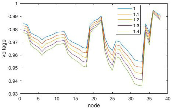
Figure 8. Voltage profiles with load variations.

5.6. Convergence Characteristics

As shown in Figure 4, the inner and outer loop usually occupy little memory, so the speed and memory of the algorithm depend mainly on the conventional power flow algorithm. For example, if the BFS method is adopted, the algorithm has a high calculation speed and requires less memory; if the NR method is adopted, due to the inverse matrix, the convergence speed will be lower than that of BFS. In addition, a reasonable estimate of the frequency and voltage deviation can accelerate the convergence. We can obtain a reasonable estimate if we neglect the power loss. Therefore, the initial value of the frequency deviation can be approximated as follows:

$$\mathsf{\Delta }f=\frac{{\displaystyle \sum _{i\in Load}}{P}_{Li}-{\displaystyle \sum _{i\in G}}{P}_{Gi}}{{\displaystyle \sum _{i\in G}}\frac{1}{m_i}}$$

(22)

Similarly, a reasonable estimate of the deviation of the virtual slack bus voltage can be obtained as

$$\mathsf{\Delta }{V}_{sb}=\frac{{\displaystyle \sum _{i\in Load}}{Q}_{Li}-{\displaystyle \sum _{i\in G}}{Q}_{Gi}}{{\displaystyle \sum _{i\in G}}\frac{1}{n_i}}$$

(23)

The convergence characteristic of the proposed method is studied for the system with 38 buses. A performance comparison was made with several existing methods using the same solver, as shown in Table 7. For the sake of fairness, all simulations were executed in a PC 64-bit Intel Core i5, 4 GB RAM.

Table 7. Comparison of convergence characteristics.

	Proposed Method $\left(\mathit{NR}\right)$	Proposed Method $\left(\mathit{BFS}\right)$	MNR [10]	DBFS [16]
Execution time (s)	0.54	0.3	0.41	0.26
Iteration times	5	5	7	4

It is shown that, although the proposed method takes into account the effect of the filter and can adapt to various control strategies, the computational time of the algorithm is comparable with other existing methods.

6. Conclusions

Considering the unique characteristics of conventional droop control inverters, this paper presents a novel method to calculate the power flow for conventional droop control DGs. The proposed method was compared using TDS, and the results showed that the proposed method can provide accurate results. Furthermore, the proposed method is universal and can handle DGs with various control strategies, including conventional droop, robust droop, constant power, and constant $Vf$. This method can also handle frequency-dependent active and reactive loads. The proposed method provides simple and accurate modifications to the conventional power flow method, and the framework of the method is generic, making it an attractive tool for power flow analysis in microgrids with different DG operating modes.

References

- Olivares, D.E.; Mehrizi-Sani, A.; Etemadi, A.H.; Canizares, C.A.; Iravani, R.; Kazerani, M.; Hajimiragha, A.H.; Gomis-Bellmunt, O.; Saeedifard, M.; Palma-Behnke, R. Trends in microgrid control. IEEE Trans. Smart Grid 2014, 5, 1905–1919. [Google Scholar] [CrossRef]
- Planas, E.; Andreu, J.; Gárate, J.I.; de Alegría, I.M.; Ibarra, E. AC and DC technology in microgrids: A review. Renew. Sustain. Energy Rev. 2015, 43, 726–749. [Google Scholar] [CrossRef]
- Asad, R.; Kazemi, A. A novel decentralized voltage control method for direct current microgrids with sensitive loads. Int. Trans. Electr. Energy Syst. 2015, 25, 197–215. [Google Scholar] [CrossRef]
- Brown, H.; Carter, G.; Happ, H.; Person, C. Z-matrix algorithms in load-flow programs. IEEE Trans. Power Appl. Syst. 1968, 87, 807–814. [Google Scholar] [CrossRef]
- Zhong, Q. Robust droop controller for accurate proportional load sharing among inverters operated in parallel. IEEE Trans. Ind. Electron. 2013, 60, 1281–1290. [Google Scholar] [CrossRef]
- Kamh, M.Z.; Iravani, R. Asequence frame-based distributed slack bus model for energy management of active distribution networks. IEEE Trans. Smart Grid 2012, 3, 828–836. [Google Scholar] [CrossRef]
- Westermann, D.; Kratz, M. A real-time development platform for the next generation of power system control functions. IEEE Trans. Ind. Electron. 2010, 57, 1159–1166. [Google Scholar] [CrossRef]
- Abdelaziz, M.M.A.; Farag, H.E.; El-Saadany, E.F.; Mohamed, A.R.I. A novel and generalized three-phase power flow algorithm for islanded microgrids using a Newton trust region method. IEEE Trans. Power Syst. 2013, 28, 190–201. [Google Scholar] [CrossRef]
- Elrayyah, A.; Sozer, Y.; Elbuluk, M. A novel load-flow analysis for stable and optimized microgrid operation. IEEE Trans. Power Del. 2014, 29, 1709–1717. [Google Scholar] [CrossRef]
- Mumtaz, F.; Syed, M.H.; Hosani, M.A.; Zeineldin, H.H. A novel approach to solve power flow for islanded microgrids using modified Newton Raphson with droop control of DG. IEEE Trans. Sustain. Energy 2016, 7, 493–503. [Google Scholar] [CrossRef]
- Caiand, N.; Khatib, A.R. A universal power flow algorithm for industrial systems and microgrids—Active power. IEEE Trans. Power Syst. 2019, 34, 4900–4909. [Google Scholar]
- Kryonidis, G.C.; Kontis, E.O.; Chrysochos, A.I.; Oureilidis, K.O.; Demoulias, C.S.; Papagiannis, G.K. Power flow of islanded AC microgrids: Revisited. IEEE Trans. Smart Grid 2018, 9, 3903–3905. [Google Scholar] [CrossRef]
- Li, C.; Chaudhary, S.K.; Savaghebi, M.; Vasquez, J.C.; Guerrero, J.M. Power flow analysis for low-voltage AC and DC microgrids considering droop control and virtual impedance. IEEE Trans. Smart Grid 2017, 8, 2754–2764. [Google Scholar] [CrossRef]
- Feng, F.; Zhang, P. Enhanced microgrid power flow incorporating hierarchical control. IEEE Trans. Power Syst. 2020, 35, 2463–2466. [Google Scholar] [CrossRef]
- Eminoglu, U.; Hocaoglu, M.H. A new power flow method for radial distribution systems including voltage dependent load models. Elect. Power Syst. 2005, 76, 106–114. [Google Scholar] [CrossRef]
- Díaz, G.; Gómez-Aleixandre, J.; Coto, J. Direct backward/forward sweep algorithm for solving load power flows in AC droop-regulated microgrids. IEEE Trans. Smart Grid 2016, 7, 2208–2217. [Google Scholar] [CrossRef]
- Hameed, F.; Hosani, M.A.; Zeineldin, H.H. A modified backward/forward sweep load flow method for islanded radial microgrids. IEEE Trans. Smart Grid 2019, 10, 910–918. [Google Scholar] [CrossRef]
- Guerrero, J.; de Vicuña, L.G.; Matas, J.; Castilla, M.; Miret, J. Output impedance design of parallel-connected UPS inverters with wireless load-sharing control. IEEE Trans. Ind. Electron. 2005, 52, 1126–1135. [Google Scholar] [CrossRef]
- Wang, Y.; Luo, A.; Jin, G. Improved robust droop multiple loop control for parallel inverters in microgrid. Trans. China Electrotech. Soc. 2015, 30, 116–123. [Google Scholar]
- Zhong, Q. Harmonic droop controller to reduce the voltage harmonics of inverters. IEEE Trans. Ind. Electron. 2013, 60, 936–945. [Google Scholar] [CrossRef]
- Xiao, F.; Zhang, C.; Duan, X.; Chen, X.; Liu, Q. Equivalence of inverter node type in power flow calculation and power flow calculation for robust droop control node. Autom. Electr. Power Syst. 2018, 42, 75–81. [Google Scholar]
- Papathanassiou, S.; Hatziargyriou, N.; Strunz, K. A benchmark low voltage microgrid network. In Proceedings of the CIGRE Symposium, Athens, Greece, 13–16 April 2005; pp. 1–9. [Google Scholar]
- Teng, J.H. A direct approach for distribution system load flow solutions. IEEE Trans. Power Del. 2003, 18, 882–887. [Google Scholar] [CrossRef]
- Ye, Q.; Mo, R.; Li, H. Multiple resonances mitigation of paralleled inverters in a solid-state transformer (SST) enabled ac microgrid. IEEE Trans. Smart Grid 2018, 9, 4744–4754. [Google Scholar] [CrossRef]
- Ramezani, M.; Li, S.; Sun, Y. Combining droop and direct current vector control for control of parallel inverters in microgrid. IET Renew. Power Gener. 2017, 11, 107–114. [Google Scholar] [CrossRef]
- Singh, D.; Misra, R.K. Effect of load models in distributed generation planning. IEEE Trans. Power Syst. 2007, 22, 2204–2212. [Google Scholar] [CrossRef]
Publisher’s Note: MDPI stays neutral with regard to jurisdictional claims in published maps and institutional affiliations. |
© 2022 by the authors. Licensee MDPI, Basel, Switzerland. This article is an open access article distributed under the terms and conditions of the Creative Commons Attribution (CC BY) license (https://creativecommons.org/licenses/by/4.0/).