Abstract
Power cable condition diagnosis and deterioration location rely on signatures of aging characteristics which precede the final breakdown. The purpose of this study was to investigate how to diagnose and locate the aging and/or deterioration of power cables through the analysis of the impedance spectroscopy. The concepts of the reference frequency and characteristic frequency of cable impedance spectroscopy are defined for the first time. Based on the reference frequency, the optimal frequency range for analysis of impedance spectroscopy can be determined, whilst based on characteristic frequency, a set of criteria for assessing cable conditions are examined and established. The solution proposed in this paper has the advantage of being easier to implement than the previously reported “broadband” impedance spectroscopy methods, as it helps to reduce the frequency range for measurement instrumentations; the proposed method also does not need the measurements of the parameters of the cable being tested.
1. Introduction
Power cables are widely used in urban transmission and distribution networks for their advantages of small footprint, high safety, and reliability [1]. At the same time, the laying environment and the ambient conditions along the cable length may vary significantly [2,3]. In different geographic segments, the rate of the aging and/or deterioration of the cable along the length may be very different, due to their non-uniform local stress level. Long-term uneven stress distribution may eventually lead to excessive local stress in the cable, resulting in insulation breakdown. Therefore, it is necessary to identify the degree of aging of the cable insulation and locate the local aging and/or deterioration before the breakdown.
The dielectric loss tangent (tan δ) is an important index measuring the energy loss of organic macromolecular materials, and it is also an important criterion for the degree of material aging [4]. In Reference [5], a viable technique for aging assessment of low-voltage cable insulation was proposed, showing the effect of the dielectric spectrum for the cable aging assessment. In Reference [6], sliced cable tests were carried out for the frequency responses of tan δ for the thermal aging and water treeing effects, and criteria were proposed for the condition assessment of medium voltage (MV) crosslinked polyethylene (XLPE) cables, using frequency domain spectroscopy. In Reference [7], accelerated thermal ageing tests were applied to XLPE pieces, and the results indicated that the lifetime for XLPE is expected to be between 40 and 60 years at 90 degrees Celsius, and the estimated cable lifetime is between 7 and 30 years for rated operating temperatures between 95 and 105 degrees Celsius. The abovementioned studies only tested specific cable samples, and each proposed its rules and criteria for accelerated aging cables. These criteria have their own limitations and have not been adopted for on-site large-scale testing.
Partial discharge (PD) is also an indicator of the weak points in cable insulation. In Reference [8], the PD behavior and accelerated aging upon repetitive DC cable energization and voltage supply polarity inversion were investigated; the results indicated that PD can occur during voltage transients that a DC cable has to withstand during its lifetime. In Reference [9], a wavelet-based PD analysis approach in noisy environments was proposed. In Reference [10], an approach to investigate the spatial distribution of plasma species related to PD dynamics in an ellipsoid void was reported. However, the detection, restoration, and localization of PD signals are still not easy tasks; especially in real-world scenarios, tiny PD signals are likely to be covered by ambient noise.
Although the application of leakage current measurement was reported for the diagnosis of cable faults, the variations in the accuracy of leakage current measurement due to operating voltage variations limited widespread use of this technique [11,12]. Methods based on time domain reflectometry (TDR) have long been applied to the detection of low impedance failures; it is ineffective to detect high impedance defects and general deteriorations [13]. Advanced signal processing techniques for improved performance in the detection of minor degradations are major challenges in employing time-frequency domain reflectometry (TFDR) techniques for the condition monitoring of cables [14]. The broadband impedance spectroscopy (BIS) technology, which does not require high voltage supplies, has received attentions in recent years. With the methods, input impedance of the cable section is measured with a sweep signal covering a wide frequency range. The characteristics of the cable impedance are dominated by the frequency-dependent parameters of the cable geometry and material, which can be used to locate cable defects. Based on the BIS principles, the Halden Reactor Project developed a method called the Line Resonance Analysis (LIRA) for cable condition monitoring [15,16]. Criterions for the assessment of cable local and global degradations were validated by experiments, but several assumptions were made in the analysis procedure, and the details of the algorithm were not published. The Inverse Fast Fourier Transform (IFFT) was introduced in the impedance spectrum analysis to acquire the location of the cable defects in References [17,18,19]. The improved method incorporates Integration Transformation (IT) into the BIS, which enhanced the localization performance by selecting an appropriate kernel function [20]. Further work illustrated the possibility of fault location in cross-bonded cables [21]. However, these broadband methods required a very high sampling rate to obtain satisfactory results, making them difficult to apply to real-world situations. The sensitivity of the input impedance was defined in Reference [22], where the scenarios considered were insufficient to establish diagnostics criteria. The Boeing Company and Brookhaven National Laboratory also developed an evaluation of BIS for electric cables used in nuclear power plants [23]; a large number of models and experimental data verified the feasibility of BIS, but it is too cumbersome for grid applications containing a far greater number of cables, as the method required the on-site measurement of cable parameters.
In the present contribution to impedance spectroscopy, the authors attempt to remove the need for measurements of real-world cables and to narrow the frequency range required for impedance spectroscopy measurement. The proposed approach mainly consists of three parts. Firstly, the transmission line parameter model of the cable is established, so as to obtain the impedance spectroscopy. Secondly the characteristic frequency in the impedance spectroscopy is developed for the identification of the different degrees and locations of aging and/or deterioration. Finally, the degree and location of the aging is determined according to the characteristic frequency of the impedance spectroscopy. The concept of the characteristic frequency of cable impedance spectroscopy is defined, for the first time, based on that; a set of criteria to assess cable conditions are examined and established for the diagnose and location of cable faults.
2. The Impedance Spectroscopy of Power Cables
2.1. Typical Structure of Power Cables
Typical structures of power cables mainly include the single-core structure and the three-core structure. The single-core structure, as presented in Figure 1, is taken as an example to study in the paper.
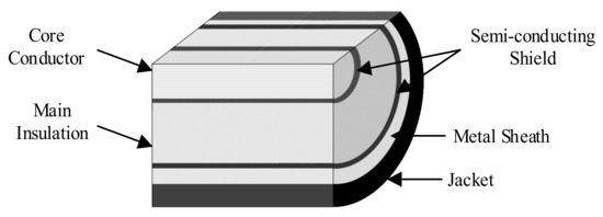
Figure 1.
A typical structure of a single-core power cable.
As shown in Figure 1, a typical single-core cable has at least six layers, namely the core conductor, inner semiconductive shielding layer (conductor shielding), main insulation, outer semiconducting shielding layer (insulation shielding), metal sheath, and jacket. There are at least two layers of metal structure, namely the core conductor and the metal sheath.
2.2. Theoretical Basis
The telegraph equation [24] based on the transmission line theory is often used to describe the relationship between the voltage, current, and electrical distance of the power transmission line, which is the result of the derivation of the transmission line model. The transmission line model treats the transmission conductor as a network formed by an infinite number of two-port circuit elements in series, as presented in (1) and Figure 2.
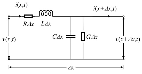
Figure 2.
A two-port distributed parameter circuit.
In (1), V and I represent the voltage and current vectors of the transmission line at electrical distance, x, respectively. Z and Y represent the impedance and admittance vectors, respectively. According to the transmission line theory, transmission lines are generally equivalent to distributed parameters, as shown in Figure 2, where R, L, C, and G represent the resistance, inductance, capacitance, and conductance per unit length of the transmission line, respectively. In the frequency domain, the current I(x) and the voltage V(x) at the electrical distance, x, of the transmission line can be presented in (2).
The general solution of (2) is shown in (3):
In (3), V+ and V− are called forward voltage waves and reflected voltage waves, respectively, and need to be determined by boundary conditions; γ and Z0 are the propagation coefficient and characteristic impedance of the transmission line, respectively, which can be presented in (4) and (5).
2.3. The Impedance Spectroscopy
The impedance spectroscopy of power cables is as a function of frequency. From (3), the impedance at the electrical distance, x, of the transmission line can be given by (6):
In (6), ΓL is the load reflection coefficient, which is shown in (7):
In (7), ZL is the load of the transmission line. If the line is open-circuited, ZL approaches infinity, and ΓL is 1.00. If the line is short-circuited, ZL approaches 0, and ΓL is −1.00. This paper mainly discusses the case of the open-circuited load.
For a typical structure of a single-core power cable, the impedance spectroscopy at the position of x = 0 can be measured by the ratio of the voltage and current between the two ends of the core conductor and the metal sheath, as presented in Figure 3. Thus, the transmission line parameters of the cable can be shown in (8)–(11).
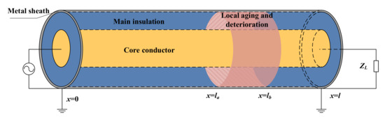
Figure 3.
The schematic diagram of local aging and deterioration of single-core cable and its measurement.
In (8), Rc is the resistance of the core conductor, Rs is the resistance of the metal sheath, r1 is the radius of the core conductor, r2 is the outer radius of the main insulation, r3 is the outer radius of the metal sheath, and ρc and ρs are the conductivity of the core conductor and the metal sheath, respectively. It is to be noted that the skin effect is neglected for the multi-conductor stranded structure of the core conductor and the hollow-circle structure for the metal sheath.
In (9), Lc and Ls are the self-inductance of the core conductor and the metal sheath, Mcs is the mutual inductance between the core conductor and the metal sheath, and μ0 is the permeability of vacuum. In (10) and (11), ε is the permittivity of the cable, ε0 is the permittivity of vacuum, A and B are fitting constants, and p is a parameter in the range of 0~1.
Earlier studies [25,26,27,28] have shown that the dielectric properties of cable insulation can be characterized by the dielectric constant, ε, which contains real and imaginary parts. The real part corresponds to the capacitive effect of the insulation, while the imaginary part represents the conductance effect of the insulation. The aging caused by various reasons (electrical, thermal, mechanical, etc.) essentially causes the molecular structure of the material to be destroyed, thereby showing different dielectric properties, which are reflected in the parameter ε. The ratio of the imaginary part to the real part of the dielectric constant is defined as the dielectric loss tangent, tan δ, also known as the loss factor. It is generally believed that the larger the tan δ value, the more serious the dielectric loss and the higher the aging degree.
2.4. Determination of Local Degradation
As shown in Figure 3, the geometry of the degradation is simplified, in this contribution, to a cylindrical ring which has the same shape as the main insulation. Thus, the location and the shape of the degradation can be defined by the x-coordinates, la and lb, and three sections being divided by the degradation. The permittivity of the degradation can be defined as εd. Then the impedance spectroscopy of the cable with local degradation can be calculated section by section. Firstly, the impedance Zb at position x = lb can be directly calculated by (6). Secondly, the impedance Za at position x = la can be calculated by taking Zb as the load. Finally, the impedance at position x = 0 can be calculated by (12).
In (12), Zb, Za, and Zs are, respectively, the impedances at position x = lb, x = la, and x = 0; Z0h and Z0d are the characteristic impedances of the health and degraded section; γh and γd are the propagation coefficients of the healthy and degraded section; and Γ1, Γ2, and Γ3 are the load reflection coefficient of each section, which can be represented by (13).
As presented in (12) and (13), the final expression of the impedance at position x = 0 is Zs, and the value of Zs is related to the position (la and lb) of the degradation and the propagation coefficients (γh and γd) of the cable. Meanwhile, the propagation coefficient, γd, is related to the dielectric constant, ε, which is an index for the aging. Therefore, the rate and location of cable aging and/or deterioration will ultimately be reflected in Zs.
3. Simulations and Results
3.1. The Impedance Spectroscopy for Healthy and Aged Cables
In order to illustrate the difference of the impedance spectroscopy between the healthy cable section and the aging part, a 20 m–long medium-voltage single-core cable was simulated, and the parameters are shown in Table 1.

Table 1.
The basic structural and material parameters of the object cable 1.
Firstly, the impedance spectroscopy of the healthy globally aged and locally aged cables at the power supply side were calculated in the range of 1 to 50 MHz. The fitting parameters (Equation (11)) for the healthy cables are, respectively, A = 2.68, B = 0.14, and p = 0.02. Namely, the relative permittivity is about 2.3, and the value of tan δ is about 4.3 × 10⁻³. Meanwhile, the fitting parameters for the aged cables are, respectively, A = 4.26, B = 0.22, p = 0.05, and la = 10 and lb = 10.01. According to (6), the impedance spectroscopy for healthy and aged cables at the position of x = 0 can be presented in Figure 4; the simulations were carried out by using MATLAB.
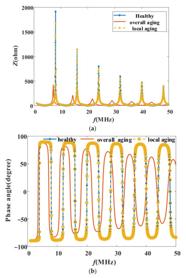
Figure 4.
The impedance spectroscopy for healthy and aged cables: (a) the impedance magnitude spectroscopy and (b) the impedance phase spectroscopy.
As shown in Figure 4, the healthy globally aged and locally aged cables have obvious differences in impedance magnitude and phase spectroscopy. In Figure 4a, the waveform of the relationship between impedance magnitude and frequency contains multiple peaks, and the peak value decreases with the increase of frequency in the range of 1~50 MHz, which is related to the length of the cable. The waveform of the overall aging slightly moves forward from the waveform of the healthy cable in frequency. The waveforms of the local aging and the healthy are very close, and the peaks of the healthy cable are slightly higher. There is a similar curve relationship in Figure 4b; however, the waveform is periodic, which depends on the length of the cable.
3.2. The Frequency Range
According to (6), the waveform of the impedance spectroscopy depends on the length of the cable. In order to obtain the complete impedance spectroscopy, the length of the cable should be greater than the wavelength of the corresponding frequency. The wavelength can be defined by (14), and the wave speed can be defined by (15):
Thus, the upper frequency limit of the impedance spectroscopy should obey (16).
In (16), fre is defined as the reference frequency of the transmission line. For the case given in Section 3.1, the upper frequency limit should be greater than 9.88 MHz, meaning that the frequency range should cover 9.88 MHz. For the convenience of subsequent description, another concept is also defined as shown in Definition 1.
Definition 1.
Characteristic frequency: The characteristic frequency is the frequency corresponding to the first peak in the impedance magnitude spectroscopy at the front end of the cable, under the condition that (16) is satisfied.
A further analysis of the expression of Zs shows that, when its denominator item is small (close to 0), the overall value of Zs is relatively large. Therefore, the characteristic frequency mainly depends on the denominator. In addition, the denominator itself is related to the rate and location of cable aging and/or deterioration, and the characteristic frequency could be used as an indicator of the aging and/or deterioration.
3.3. The Location for Local Degradation
As presented in Figure 4, the waveform showed multiple peaks between the impedance magnitude and the frequency; the value and the position of the peaks changes when the degradation occurs. Here, the frequency of the first peak is defined as the characteristic frequency. If the position of the degradation la is set to 1~19 m and the length of the degradation is set to 0.01 m, the impedance magnitude spectroscopy can be presented as shown in Figure 5.
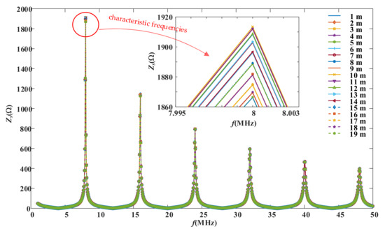
Figure 5.
The impedance magnitude spectroscopy with the characteristic frequencies for the position of the degradation at 1~19 m.
As shown in Figure 5, the values of the impedance magnitude at the characteristic frequencies are quite different at different degradation positions. The relationship between the impedance magnitude and the location of degradation, measured as the distance from the front end of the cable, can be presented as shown in Figure 6.
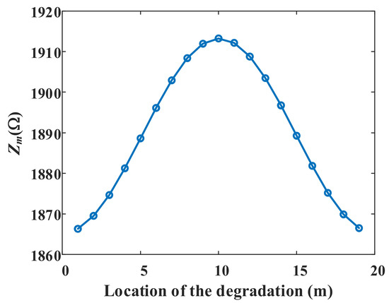
Figure 6.
The relationship between the impedance magnitude at the characteristic frequency and the location of the degradation.
3.3.1. Fault Location for Different Cable Lengths
In Figure 6, the impedance first increases and then decreases with the distance of the degradation, and the maximum value appears at the midpoint. Simulations were also carried out for longer cables, at lengths such as 50 m, 100 m, 1000 m, 10,000 m, and still with a resolution of the degradation point of 0.1 mm. The results are shown in Figure 7.
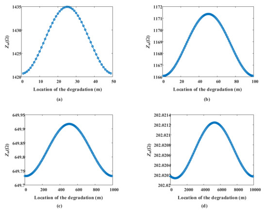
Figure 7.
The relationship between the impedance magnitude at the characteristic frequency and the position of the degradation for (a) 50 m, (b) 100 m, (c) 1000 m, (d) 10,000 m cables.
It is to be noted that the reference frequency, fre, decreases with the length of the line. The frequency range of the impedance spectroscopy will also be smaller for longer cables. Thus, the distinction of Zm also decreases with the length in Figure 7, which indicates that the measurement resolution of the impedance should increase with the length.
3.3.2. The Location for Different Degrees of the Degradation
As mentioned in Section 2.3, the degree of the degradation can be characterized by the dielectric constant or the value of tan δ. In order to locate the degradation of different degrees, simulations were carried out for nine different degrees of degradation, as shown in Table 2 and Figure 8.
Table 2.
Parameters of different degrees of the degradation.
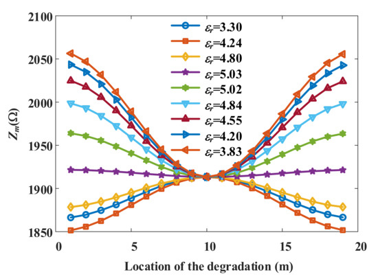
Figure 8.
The relationship between the impedance magnitude at the characteristic frequency and the position of the degradation with different aging degrees.
In order to show the effect of aging more comprehensively, the parameters in Table 2 are slightly exaggerated. It is to be noted that the value of tan δ increases with the increase of the ε parameters, while the relative permittivity does not, meaning that the real and imaginary parts of the permittivity do not vary linearly with the ε parameters. This is not common in practice. The aging in engineering practice tends to have a greater impact on the imaginary part of the permittivity; that is, the higher the aging degree, the greater the value of tan δ and the greater the value of the relative permittivity. In the simulation, extreme cases where the value of tan δ and the value of the relative permittivity do not change synchronously are also considered. In Figure 8, if the value of tan δ and the value of the relative permittivity change synchronously, the relationship curve of Zm and the location of the degradation shows an upwardly convex; otherwise, the curve is downwardly concave. In general, the position of the degradation can be deduced by the Zm value, but this approach produces a false solution at around midpoint, due to symmetry. Experienced engineers can make further judgments based on the actual situation on site, such as water soaking, skin damage, corners, etc. More discussions can be found in Section 5. It is also to be noted that the impedance symmetry around the midpoint also appeared in Figure 8. Mathematically, this is due to the piecewise calculation method used in the paper, as shown in (12) and (13). Another explanation is that the impedance of the cable exhibits extreme values at the characteristic frequency. For local aging, if the position is just at the midpoint of the cable, and the impedance measurement position is at the front end, the distance from the front end to the midpoint of the line for one reflection would be exactly the complete line length. In this case, the first half is in a healthy state and has nothing to do with the degree of aging; the impedance at the characteristic frequency of the special position is also independent of the degree of aging.
3.3.3. The Location for Different Local Degradation Sizes
As mentioned in Section 2.4, the shape of the degradation is simplified to a cylindrical ring so that the size of the degradation can be defined by the length. Simulations were carried out for nine different lengths of the degradation, namely 0.01~0.09 m. Moreover, the fitting parameters for the aged cables are still, respectively, A = 4.26, B = 0.22, and p = 0.05; the results are shown in Figure 9.
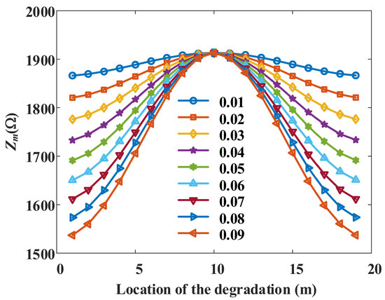
Figure 9.
The relationship between the impedance magnitude at the characteristic frequency and the position of the degradation for different physical sizes of local degradation.
As presented in Figure 9, the size of the degradation mainly affects the scale of the relationship curve of Zm and the location of the degradation. As the physical size of the degradation increases, the curve becomes steeper; in the meantime, it becomes easier for the location. The same as in Figure 8, the position of the degradation can be deduced by the Zm value, but this approach also produces a false solution that is symmetric about the midpoint. More discussions can be found in Section 5.
4. The Criterion for the Diagnosis and Location
The results presented in Section 3 indicated that the impedance spectroscopy, especially the characteristic frequency, can be used for the diagnosis and location of cable aging and deterioration. The procedure of diagnosis and location of general aging and local deterioration can be summarized as shown in Figure 10.
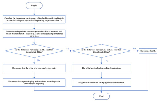
Figure 10.
The schematic diagram of the procedure for diagnosis and location of cable fault.
The parameters of a cable under healthy condition can be obtained by calculation and measured, respectively. Contrasting characteristic frequencies can distinguish the overall aging cable from the ones containing other types of deteriorations. The differences in impedance values can help determine whether and where the cable has local aging and/or deterioration. As presented in Figure 10, the first step is to calculate cable impedance spectroscopy to obtain its characteristic frequency, fch, and corresponding impedance value, Zmh, under healthy condition. The second step is to measure the impedance spectroscopy of the cable and obtain its characteristic frequency, fcO, and corresponding impedance value, ZmO. The third step is to determine whether the difference between fch and fcO is less than the calculated deviation. If the difference is greater than the established criterion of deviation, the cable is in an overall aging state. Then the degree of aging can be determined according to the characteristic frequency. If the difference is less than the deviation, the next step is to determine whether the difference between Zmh and ZmO is less than the calculated deviation. If the difference is greater than the calculated deviation, the cable has local aging and/or deterioration. If the difference is less than the deviation indicated in the criterion, the cable is healthy.
Therefore, the key to applying this method is knowing the length of the cable and the frequency range of the impedance spectroscopy. For the overall aging, as an example, the degrees of aging are shown in Table 3; the corresponding impedance spectroscopy can be shown in Figure 11.
Table 3.
The different degrees of the aging.
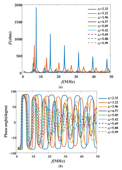
Figure 11.
The impedance spectroscopy for the cables of different aging degrees: (a) the impedance magnitude spectroscopy and (b) the phase angle of the impedance spectroscopy.
As presented in Figure 11, there is a clear distinction between both impedance magnitude and phase spectroscopies for healthy and overall aged states. For the impedance magnitude spectroscopy, as shown in Figure 11a, the distinction is mainly reflected in the characteristic frequency and impedance; the characteristic frequency and corresponding impedance magnitudes change with the aging degree. For the impedance phase spectroscopy, as shown in Figure 11b, the distinction is mainly reflected in the periodicity observed in the curve. As the aging degree increases, the phase-angle change period and the amplitude also change. It is to be noticed that the phase-frequency period of the impedance spectroscopy becomes shorter as the aging degree increases, meaning that excessive aging will affect the appropriate frequency range of the impedance spectroscopy. However, the degree of aging is not known before the measurement, and the probability of serious overall aging is also very low; the selection of the frequency range does not change due to the different degrees of aging.
The criterion for the overall aging can be based on the relationship curve between the aging degree and the characteristic frequency with its impedance value, as shown in Figure 12.
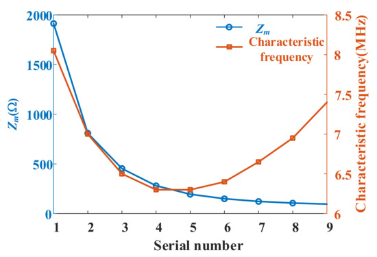
Figure 12.
The relationship between the degree of aging and the characteristic frequency with its impedance value.
In Figure 12, nine cable samples with different degrees of aging were simulated; as the aging degree increases, the characteristic frequency first decreases and then increases, and the corresponding impedance value keeps decreasing. Therefore, through the set of curves, the degree of aging expressed in terms of relative permittivity and/or tan δ value can be inferred. Therefore, the characteristic frequency with its impedance value can be the criterion for the diagnosis and location of the local aging and/or degradation.
5. Discussion
The results of the impedance spectroscopy indicate that the analysis of characteristic frequency and impedance spectroscopy can be used to set up criteria for cable condition diagnosis and location. It is also noted that the cable length and the frequency range affect the resulting curves of the impedance spectroscopy, which further affects important parameters such as characteristic frequency. This section further discusses the frequency range and the advantages of the proposed method.
5.1. The Frequency Range
In Section 3.2, the reference frequency and the characteristic frequency were defined according to the transmission line theory, and they both related to the cable length. The characteristic frequency is also related to the rate of the aging and/or deterioration, and it is used as an index for the aging and/or deterioration. The reference frequency is related to the healthy state, and it is used as an index for the selection of the upper limit of frequency range to be measured. The upper limit of the frequency range is set as an integer value of 4~5 times the reference frequency, which is convenient for selection in actual measurement, and the lower limit is an integer value that is about an order of magnitude smaller than the reference frequency.
Since the reference frequency should be calculated from the electrical parameters of a cable under healthy state, it also seems necessary to adjust the frequency range if the aging of the actual measurements becomes excessively high. For example, for the following groups of aging parameters in Table 2, the real characteristic frequency may be missed if the frequency range of 1~50 MHz were to be selected, and it is necessary to appropriately reduce the lower limit frequency.
For the location of the degradation, the same impedance value in the measurement may correspond to two different positions, as shown in Figure 6 and Figure 7, and the two positions are symmetrical about the midpoint. Meanwhile, the relationship between the impedance magnitude at the characteristic frequency and the position of the degradation could be monotonous if the upper limit of the frequency range is less than a half of the reference frequency. In that case, the impedance magnitude at the characteristic frequency could be replaced by the impedance magnitude at the lower limit frequency. However, the consequence is that the resolution requirements for the impedance magnitude will be greatly improved, as shown in Figure 13.
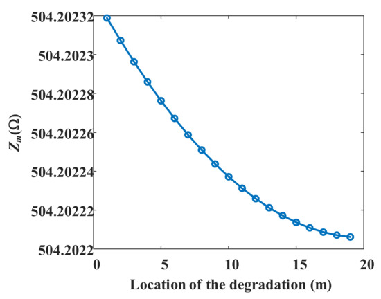
Figure 13.
The monotonous relationship between the impedance magnitude at the characteristic frequency with respect to the position of the degradation.
5.2. The Advantages of the Proposed Method
The proposed method has two main functions: one is to diagnose the aging condition of the cable insulation, and the other is to locate the local aging deterioration. It naturally combines the functions of condition diagnosis and fault location and is, in principle, different from other methods of condition diagnosis and the method of fault location. Specifically, the method mainly targets aging and/or deterioration.
To the authors’ knowledge, there have also been studies [20,21,22,23] on the aging diagnosis and location of power cables based on the impedance spectroscopy. The main difference between the proposed method with those is in the nature of the location criterion. In References [20,21,22], the deterioration was located through the Integration Transformation (IT). The key to the earlier reported method is the IT function, which is also known as the kernel function. Theoretically, the kernel function should not be a fixed function, and its selection should depend on the actual cable parameters; this method did not show consistent results under different cable parameters. In Reference [23], the deterioration was located through the phase angle of the impedance spectroscopy δ(ω), and the accurate location results could only be achieved when the real-world cable parameters are available, which requires accurate on-site testing of the line parameters in advance. It is achievable for nuclear power plants—as this was their research object—having relatively few power cables. However, this is almost impossible for grid companies that contain a massive number of and much lengthier power cables. A comparison of the condition diagnosis and location methods is presented in Table 4.
Table 4.
The comparison of the condition diagnosis and location methods.
The main innovation of the proposed method is that the concepts of the reference frequency and the characteristic frequency of cable impedance spectroscopy were proposed. The reference frequency provides a reference for the test range of the impedance spectroscopy, so that cable operation and maintenance personnel can choose the best range of measurement frequency, not necessarily “broadband”. The characteristic frequency is the main criterion for condition diagnosis and location. It does not require transformation in space and frequency domains, nor the additional of parameter testing, thus making the method more convenient to use.
6. Conclusions
In the paper, a novel method for diagnosing and locating aging and deteriorating power cables based on the analysis of reference and characteristic frequencies of the impedance spectroscopy was proposed. The reference frequency was defined and calculated to aid in determining the frequency range when carrying out the impedance spectroscopy. While the frequency corresponding to the first peak of the impedance magnitude–frequency curve is defined as the characteristic frequency. Then the characteristic frequency is used to establish the criteria for the diagnosis and location of cable aging and local defects, based on results of simulation studies. In the proposed method, the overall aging, its aging degree, the local aging and/or deterioration, and its degree and location can be determined step by step. Compared with the traditional aging diagnosis, the advantage of the solution proposed in this paper is that it is easier to implement comparing with many previous efforts where lab tests of electrical and mechanical properties are required on cable samples with artificial defects. Compared with earlier impedance spectroscopy methods, this contribution is more convenient to apply, as it does not require the measurement of cable parameters, and it helps to narrow the range of measurement frequency required.
Author Contributions
Conceptualization, C.Z. and M.L.; methodology, M.L.; data analysis, G.L. and M.L.; writing—original draft preparation, G.L. and M.L.; writing—review and editing, W.Z. and C.Z.; supervision, C.Z.; project administration, J.C.; funding acquisition, J.C., H.L. and L.H. All authors have read and agreed to the published version of the manuscript.
Funding
This research was funded by STATE GRID Corporation of China, grant number 5700-202118195A-0-0-00.
Institutional Review Board Statement
Not applicable.
Informed Consent Statement
Not applicable.
Data Availability Statement
Not applicable.
Conflicts of Interest
The authors declare no conflict of interest.
References
- Zhou, C.; Yi, H.; Dong, X. Review of recent research towards power cable life cycle management. High Volt. 2017, 2, 179–187. [Google Scholar] [CrossRef]
- Fabiani, D.; Mazzanti, G.; Suraci, S.V.; Diban, B. Innovative Development and Application of a Stress-Strength Model for Reliability Estimation of Aged LV Cables for Nuclear Power Plants. IEEE Trans. Dielectr. Electr. Insul. 2021, 28, 2083–2090. [Google Scholar] [CrossRef]
- Montanari, G.C.; Hebner, R.; Morshuis, P.; Seri, P. An approach to insulation condition monitoring and life assessment in emerging electrical environments. IEEE Trans. Power Deliv. 2019, 34, 1357–1364. [Google Scholar] [CrossRef]
- Hedir, A.; Moudoud, M.; Lamrous, O.; Rondot, S.; Jbara, O.; Dony, P. Ultraviolet radiation aging impact on physicochemical properties of crosslinked polyethylene cable insulation. J. Appl. Polym. Sci. 2020, 137, 48575. [Google Scholar] [CrossRef]
- Fabiani, D.; Suraci, S.V. Broadband Dielectric Spectroscopy: A Viable Technique for Aging Assessment of Low-Voltage Cable Insulation Used in Nuclear Power Plants. Polymers 2021, 13, 494. [Google Scholar] [CrossRef]
- Jahromi, A.N.; Pattabi, P.; Densley, J.; Lamarre, L. Medium voltage XLPE cable condition assessment using frequency domain spectroscopy. IEEE Electr. Insul. Mag. 2020, 36, 9–18. [Google Scholar] [CrossRef]
- Alghamdi, A.S.; Desuqi, R.K. A study of expected lifetime of XLPE insulation cables working at elevated temperatures by applying accelerated thermal ageing. Heliyon 2020, 6, e03120. [Google Scholar] [CrossRef] [Green Version]
- Montanari, G.C.; Seri, P.; Bononi, S.F.; Albertini, M. Partial discharge behavior and accelerated aging upon repetitive DC cable energization and voltage supply polarity inversion. IEEE Trans. Power Del. 2021, 36, 578–586. [Google Scholar] [CrossRef]
- Mor, A.R.; Munoz, F.A.; Wu, J.; Heredia, L.C.C. Automatic partial discharge recognition using the cross wavelet transform in high voltage cable joint measuring systems using two opposite polarity sensors. Int. J. Electr. Power Energy Syst. 2020, 117, 105695. [Google Scholar]
- Algwari, Q.T.; Saleh, D.N. Numerical Modeling of Partial Discharge in a Void Cavity Within High-Voltage Cable Insulation. IEEE Trans. Plasma Sci. 2021, 49, 1536–1542. [Google Scholar] [CrossRef]
- Dong, X.; Yang, Y.; Zhou, C.; Hepburn, D.M. Online Monitoring and Diagnosis of HV Cable Faults by Sheath System Currents. IEEE Trans. Power Del. 2017, 32, 2281–2290. [Google Scholar] [CrossRef]
- Yang, Y.; Hepburn, D.M.; Zhou, C.; Zhou, W.; Bao, Y. On-line monitoring of relative dielectric losses in cross-bonded cables using sheath currents. IEEE Trans. Dielectr. Electr. Insul. 2017, 24, 2677–2685. [Google Scholar] [CrossRef] [Green Version]
- Shi, Q.; Troeltzsch, U.; Kanoun, O. Detection and localization of cable faults by time and frequency domain measurements. In Proceedings of the 7th International Multi-Conference on Systems, Signals and Devices, Amman, Jordan, 27–30 June 2010; pp. 1–6. [Google Scholar]
- Shi, Q.; Kanoun, O. A new method of locating the single wire fault. In Proceedings of the 12th International Conference on Signal Processing (ICSP), HangZhou, China, 26–30 October 2014; pp. 2262–2267. [Google Scholar]
- Fantoni, P.F.; Toman, G.J. Cable Aging Assessment and Condition Monitoring Using Line Resonance Analysis (LIRA); American Nuclear Society—ANS: La Grange Park, IL, USA, 2006; Volume 12, pp. 177–186. [Google Scholar]
- Maier, T.; Lick, D.; Leibfried, T. Frequency-Domain Cable Model with a Real Representation of Joints and Smooth Failure Changes and a Diagnostic Investigation with Line Resonance Analysis. In Proceedings of the 2018 Condition Monitoring and Diagnosis (CMD), Perth, Australia, 23–26 September 2018; pp. 1–6. [Google Scholar]
- Ohki, Y.; Hirai, N. Effects of the structure and insulation material of a cable on the ability of a location method by FDR. IEEE Trans. Dielectr. Electr. Insul. 2016, 23, 77–84. [Google Scholar] [CrossRef]
- Hirai, N.; Ohki, Y. Highly sensitive detection of distorted points in a cable by frequency domain reflectometry. In Proceedings of the International Symposium on Electrical Insulating Materials, Niigata City, Japan, 1–5 June 2014; pp. 144–147. [Google Scholar]
- Yamada, T.; Hirai, N.; Ohki, Y. Improvement in sensitivity of broadband impedance spectroscopy for locating degradation in cable insulation by ascending the measurement frequency. In Proceedings of the International Conference on Condition Monitoring and Diagnosis, Bali, Indonesia, 23–27 September 2012; pp. 677–680. [Google Scholar]
- Zhou, Z.; Zhang, D.; He, J.; Li, M. Local degradation diagnosis for cable insulation based on broadband impedance spectroscopy. IEEE Trans. Dielectr. Electr. Insul. 2015, 22, 2097–2107. [Google Scholar] [CrossRef]
- Mo, S.; Zhang, D.; Li, Z.; Wan, Z. The Possibility of Fault Location in Cross-Bonded Cables by Broadband Impedance Spectroscopy. IEEE Trans. Dielectr. Electr. Insul. 2021, 28, 1416–1423. [Google Scholar] [CrossRef]
- Pan, W.; Li, X.; Zhu, Z.; Zhao, K.; Xie, C.; Su, Q. Detection Sensitivity of Input Impedance to Local Defects in Long Cables. IEEE Access 2020, 99, 55702–55710. [Google Scholar] [CrossRef]
- Rogovin, D.; Lofaro, R. Evaluation of the Broadband Impedance Spectroscopy Prognostic/Diagnostic Technique for Electric Cables Used in Nuclear Power Plants. U.S Nuclear Regulatory Commission. Available online: https://www.nrc.gov/reading-rm/doc-collections/nuregs/contract/cr6904/cr6904.pdf (accessed on 18 July 2022).
- Wedepohl, L.M.; Wilcox, D.J. Transient analysis of underground power-transmission systems. System-model and wave-propagation characteristics. Proc. Inst. Electr. Eng. 1973, 120, 253–260. [Google Scholar] [CrossRef]
- Teng, C.; Zhou, Y.; Zhang, L.; Zhang, Y.; Huang, X.; Chen, J. Improved electrical resistivity-temperature characteristics of insulating epoxy composites filled with polydopamine-coated ceramic particles with positive temperature coefficient. Compos. Sci. Technol. 2022, 221, 109365. [Google Scholar] [CrossRef]
- Said, A.; Ghunem, R.A. A Techno-Economic Framework for Replacing Aged XLPE Cables in the Distribution Network. IEEE Trans. Power Del. 2020, 35, 2387–2393. [Google Scholar]
- Arikan, O.; Uydur, C.C.; Kumru, C.F. Prediction of dielectric parameters of an aged mv cable: A comparison of curve fitting, decision tree and artificial neural network methods. Electr. Power Syst. Res. 2022, 208, 107892. [Google Scholar] [CrossRef]
- Paramane, A.; Chen, X.; Dai, C.; Guan, H.; Yu, L.; Tanaka, Y. Electrical insulation performance of cross-linked polyethylene/MgO nanocomposite material for ±320 kV high-voltage direct-current cables. Polymer Compos. 2020, 41, 1936–1949. [Google Scholar] [CrossRef]
- IEC 60287-1-1:2006+A1:2014; Electric Cables—Calculation of the Current Rating—Part1-1: Current Rating Equations (100% Load factor) and Calculation of Losses—General. International Electrotechnical Commission: Geneva, Switzerland, 2014.
Publisher’s Note: MDPI stays neutral with regard to jurisdictional claims in published maps and institutional affiliations. |
© 2022 by the authors. Licensee MDPI, Basel, Switzerland. This article is an open access article distributed under the terms and conditions of the Creative Commons Attribution (CC BY) license (https://creativecommons.org/licenses/by/4.0/).