Abstract
For two decades, the Thai government has been promoting ethanol and biodiesel consumption through tax measures and price subsidies. Although this policy has substantially increased the consumption and production of biofuels, there is concern regarding its future fiscal burden. Due to fiscal constraints, the Thai government has planned to completely terminate the biofuel subsidy by 2022. This study aims at examining the economy-wide impacts of removing the biofuel subsidy and also conducting simulations of alternative scenarios, i.e., improving the yield of energy crops and reallocating the burden to expand capital investment in energy crop plantations. A recursive dynamic computable general equilibrium (CGE) model was used as the main quantitative method to conduct four simulation scenarios. This model was validated by comparing the simulation results with the actual 2015–2019 data and showed low values of root mean square error (RMSE). The simulation results indicate that solely terminating the price subsidy would lead to economy-wide contraction. Meanwhile, eliminating the price subsidy along with influencing crop yield improvement and expanding capital investment in energy crop plantations would lead to the lowest negative impacts. Therefore, the termination of the price subsidy should be simultaneously implemented with supply-side expansions.
1. Introduction
Given the scarcity of fossil energy resources, Thailand must import an enormous amount of energy, i.e., over 60% of its total domestic energy consumption annually [1], which results in a substantial economic loss every year. Consequently, the Thai government has placed importance on renewable energy development to replace fossil energy, especially biofuels used in the transportation sector. For over two decades, the government has driven biofuel production and consumption via tax measures and pricing policy, especially biofuel subsidies using an oil fund [2]. The production of purified biofuel (ethanol and biodiesel) is costly [3,4]; therefore, a subsidy aims at maintaining biofuel prices lower than fossil fuel prices. The government uses the subsidy to offset the costs of biofuel feedstocks through petroleum refineries to farmers. As a result, energy crop farmers are indirect beneficiaries of the oil fund [5]; however, to compensate for biofuel prices, the government must provide a considerable budget, which, inevitably, affects the liquidity of the oil fund.
Consequently, the current government decided to revise and issue the new State Oil Fund Act B.E. 2562 (2019), which distinctly determines the oil fund allocation to occasionally stabilize domestic fuel prices during unusual situations (e.g., oil price shocks in the global market). Additionally, the government has planned to completely eliminate biofuel subsidies by 2022 [6]. Removing the biofuel subsidy triggers multidimensional concerns involving formulating an appropriate energy policy that would be effective after 2022.
Figure 1 shows an example of the biofuel price structure of Thailand. The graph indicates that four biofuel types have been moderately subsidized. The biofuels sold in Thailand are categorized as biodiesel and gasohol. There are three types of biodiesel, namely H-Diesel (mandatory), H-Diesel B7 (option), and H-Diesel B20 (option for heavy trucks). Gasohol is classified as Gasohol 91, Gasohol 95 (E10), Gasohol 95 (E20), and Gasohol 95 (E85) [7]. Retail prices comprise ex-refinery or producer prices, excise tax, municipal tax, oil fund levy, energy conservation fund, value-added tax (VAT) on the oil producer (VAT1), marketing margins, and value-added tax on the oil trader (VAT2). The negative value of the oil fund means the fuels are subsidized, including Gasohol 95 (E20), Gasohol 95 (E85), H-Diesel, and H-Diesel B20. If the subsidy is removed, the retail prices would increase correspondingly, therefore inducing higher production costs, household expenditures, and other costs of economic activities.
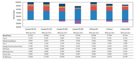
Figure 1.
Biofuel price structure with the oil subsidy shown in purple.
In general, removing the biofuel subsidy would have both negative and positive economy-wide implications, i.e., on the one hand, removal of the subsidy would decrease the oil fund budget for offsetting biofuel prices, while, on the other hand, the government would experience a budget savings, thereby lowering the fiscal burden and/or allowing alternative options for fiscal expenditures. Studying the effects caused by such policy change requires a structural model that can capture the economy-wide propagations and ultimate impacts. A computable general equilibrium (CGE) model is a tool widely used for this purpose. A CGE model comprises the interrelationships among economic agents. Changes in some variables in the model can concurrently affect other agents in the economy. Therefore, a CGE model is an appropriate approach for policy study [8], especially the nationwide impacts of fuel subsidies.
Conventionally, investment is an essential factor that drives economic growth because it leads to an increase in employment in the short term and improves productivity by strengthening production sectors in the long term. For Thailand, the average TFP growth (for 2015–2018) was 1.6% [9]. In addition, considering the agriculture sector, its average TFP growth was only 0.68% per annum [10]. Therefore, improving the TFP growth is necessary for Thailand because it would significantly lead to an improved GDP and higher population income.
On the basis of the description above, in this study, we focus on three policy options, namely (1) elimination of biofuel subsidy, (2) reallocation of the biofuel subsidy to investments in energy crop plantations, and (3) TFP enhancement of energy crops. Therefore, to achieve the results of the counterfactual experiments of three policy regimes, in this study, we apply the CGE model to address the structure of the Thai economy and examine the impacts on the economic system.
2. Literature Review
Many previous studies have used a CGE model to analyze reforming energy subsidy, and have revealed that imposing a price distortion mechanism can cause inefficient resource allocations [11,12]. A study regarding Malaysia stated that, on the one hand, removing energy subsidies would increase the real GDP and real investment and would also decrease total energy demand, which would be beneficial to the economy. On the other hand, removal of energy subsidies would lead to a decrease in household consumption and welfare. As a result, their CGE-based simulation result recommended that the Malaysian government redistribute the budget to mitigate household effects [13]. Similarly, a study in Yemen revealed that although subsidy reduction would lead to economic growth, it would induce poverty expansion, and authors therefore suggested the government should transfer income to critical economic activities, such as the poorest households and public investments to enhance productivity and eliminate harmful effects [14].
In China, removal of the fossil fuel subsidies could result in negative consequences on output, potential competitiveness, energy demand, emission, and economic growth [15]. Given that subsidy removal could induce positive and negative effects, policies should focus on reallocating resources from the price subsidy to alternative measures [16]. In particular, using a structural model to simulate all possible scenarios generated by packages of regimes is necessary for formulating the optimal energy policy [17].
In Thailand, the oil fund mainly receives income from an oil levy, which is subsequently reallocated to subsidize domestic prices of various fuels. Regarding the fund’s sustainability, several CGE-based studies related to energy taxes and subsidies have been conducted. The Asian Development Bank (ADB) has recommended that the Thai government remove the subsidy from fossil fuels and use it sporadically for mitigating world oil price fluctuations [1]. Another study has stated that, although eliminating the oil fund would lead to a lower GDP in the short term, the GDP growth would recover in the long term [18]. This study also indicated that, although the oil fund has been used for the biofuel subsidy to promote green energy, it has ignited energy market intervention. The results of terminating the subsidy would be similar to an increase in tax. If the government removes the biofuel subsidy, it would lower the GDP, social welfare, and energy consumption [5].
The above-mentioned studies have only analyzed the effects of tax and subsidy reforms. Another perspective involves investigating the benefits of a subsidy swap. Given that the removal of biofuel subsidies would mean that the government would retain more savings, some studies have suggested that some of the increased government savings should be reallocated [19]. Specifically, instead of freezing additional government savings earned from removing subsidies, the government should allocate the budget to investments in essential projects or compensation for people who face adverse effects [20]. According to these suggestions, the swap concept recommends that the government reallocate fossil energy subsidies to clean energy investments to expand economic growth; however, the results from reallocations vary by the area of study. An Indonesian study reported that eliminating energy subsidies and transferring money to invest in infrastructure and the renewable energy industry would positively impact the economy [21]. As shown by a study in South Africa, a decrease in the fuel subsidy and reallocating budgets to support public transportation would positively impact the economy [22]. In the case of Iran, eliminating energy subsidies and redistributing the budget to households and production sectors would result in a decrease in the GDP and higher inflation [23]. Given the diversity of national impacts, incorporating a combination of regimes in Thailand’s policy on subsidy elimination is crucial to the country’s development progress.
3. Methodologies
The model utilized in this study was adapted from a standard recursive dynamics CGE model published by the Partnership for Economic Policy (PEP) [24]. The procedures for constructing this model to simulate the economy-wide impacts in Thailand are explained in the following subsections.
3.1. Database
The data showed that the interactions among economic agents in the CGE model were the social accounting matrix (SAM). The SAM was an economic accounting of income and expenditure developed from the Input-Output (I/O) table, provided by Thailand’s Office of the National Economic and Social Development Council [25]. This study incorporated new sectors and commodities for the energy policy analysis by using databases from various sources of Thailand, such as the Office of Energy and Policy Planning (EPPO), Department of Alternative Energy Development and Efficiency (DEDE), Department of Energy Business (DEB), Bank of Thailand (BOT), the Office of Agricultural Economics (OAE), and the Thailand Research Fund (TRF) [7,26,27,28,29,30].
The new SAM was comprised of 35 production sectors, 42 commodities (listed in Table A1 of Appendix A), and 3 institutes, i.e., the household, the government, and the rest of the world. There were two industries that produce multiple commodities: the petroleum refinery and sugar production industries. The petroleum sector was split into petroleum products, i.e., liquefied petroleum gas, jet oil and kerosene, gasohol, biodiesel, fuel oil, and other petroleum products. Given the deceleration of gasoline production and consumption, in this study, gasoline was combined with gasohol E10, whereas gasohol E20 and gasohol E85 were combined as gasohol E20/E85. Similarly, the type of biodiesel typically relies on government determination. This study separated biodiesel into biodiesel (mandatory) and biodiesel (option). The mandatory biodiesel was B5, whereas the optional biodiesel was combined with B7 and B10. Sugar production typically produces sugar products and molasses. Alternatively, ethanol can be produced by two industries, namely molasses-based ethanol production and cassava-based ethanol production. Although ethanol production in Thailand can be produced directly from sugar cane, this rarely occurs because sugar cane is much more suited for food manufacturing than energy.
3.2. Model Structure
Figure 2 shows the nested production structure in the model. At the top level, the production is a fixed proportion between the primary and the intermediate factor following the Leontief production function (LEO). At the next level, labor and capital are merged with constant elasticity of substitution (CES) (The values of elasticity of substitution parameters are exhibited in Appendix A). At the same level, the total intermediate commodity is the integration between mixed gasohol, mixed biodiesel, and other commodities using the LEO. At the lowest level, there are two combinations of CES: mixed biodiesel comprises mandatory biodiesel and optional biodiesel, while gasohol is the combination of gasohol (E10) and gasohol (E20/E85).
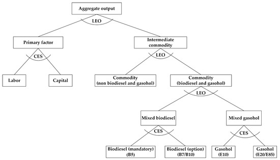
Figure 2.
Nested production structure.
Regarding the other relationships in the model, household consumption aimed to maximize utility subjected to budget constraints following a Stone–Geary utility function. The investment demand varied inversely with commodity price. International trading was the substitution between commodity produced domestically and exports with constant elasticity of transformation (CET) (The values of elasticity of transformation parameters are shown in Appendix A). Similarly, the optimal selection between an import and the domestic commodity was determined by a function of constant elasticity of substitution.
3.3. Dynamics Assumption
This study emphasized a short-term period of ten years (2022–2031). As introduced by the Partnership for Economic Policy (PEP) [24], the recursive-dynamic mechanism was applied to the model because it allowed the intertemporal relationship between investment and capital stock. (Alternatively, the intertemporal mechanism of the CGE model can be fully dynamic. For example, the mathematical specifications can be extended to include the fully endogenized processes of intertemporally optimizing behaviors [31,32]). Also, this specification enabled the values of variables jointly involved in the dynamic adjustment to be exogenously defined based on the reports and official projections. Hence, these parameters were exogenously assigned to increase over time (The values of these exogeneous variables are shown in Appendix A), i.e., population, export, total investment, public investment, government expenditures, productivity, depreciation rate, and the elasticity of investment demand. The population growth was adapted from the Organization for Economic Co-operation and Development (OECD) and the International Labor Organization (ILO) [33]. The export, total investment, public investment, and government expenditures were based on the national income account reported by the Office of the National Economic and Social Development Council [34]. The productivity was averaged from the total factor of productivity reported by the OIE [35]. The depreciation rate and the elasticity of investment demand were applied from the previous studies [36,37].
3.4. Closure and Solution
The relationship among variables in the CGE model was comprised of more equations than variables. Therefore, some variables were fixed and denoted as exogenous variables to solve unique solutions that satisfy the Walras law [38]. In this study, the exogenous variables were government expenditures, public sector investment, total investment, capital stock, minimum consumption, labor supply, stock change, and world prices of imports and exports. The numeraire was an exchange rate. The scale, share, and exponential parameters were calibrated, following the methods introduced in previous studies [37]. The general algebraic modeling system (GAMS) was used to solve equations for equilibrium using a constrained nonlinear system (CNS).
3.5. Scenarios
The Thai government aims to remove the biofuel subsidy, which is an enormous burden on the oil fund. In this study, we attempt to examine new measures for increasing benefits that could oppose the negative effects caused by higher biofuel prices. The new measures emphasize TFP and investments in energy crop plantations, which are upstream of the biofuel supply chain.
Figure 3 illustrates a flowchart for the reallocation of biofuel subsidy. The government levies all petroleum taxes, including excise tax, municipal tax, oil fund, energy conservation, and two value-added taxes (refinery and oil trading). The oil fund has been used to offset the purified biofuel prices. In this study, if the subsidy is removed, the government receives more income and savings. Then, it can reallocate some of its budget to invest in energy crop plantations, as shown in Table 1. All scenarios involved complete removal of the biofuel subsidy. Scenario A (SIM A) had no reallocation of biofuel subsidy to investment and no change in TFP. SIM B had no reallocations but enhanced TFP by 1%. SIM C reallocated 10% of the biofuel subsidy to investment in energy crop plantations (e.g., sugar cane, cassava, and oil palm), but it had no change in TFP. Finally, SIM D reallocated 10% of the biofuel subsidy to investment in energy crop plantations and enhanced TFP by 1%.
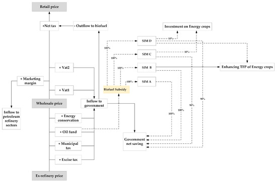
Figure 3.
Recycle flow chart of biofuel subsidy into supply-sided expansion for Scenarios A–D (SIMs A–D).

Table 1.
The four scenarios used for simulations.
The percentage changes in TFP are based on a previous study that reported Thailand had an increase in TFP of agriculture by less than 1% [39]. In addition, given that there have been no previous studies on energy crop investments, this study applied a policy scenario simulation ranging from no reallocation to reallocation when the subsidy elimination is effective. To explore long-term impacts, the model used in this study was based on the recursive dynamic approach. Therefore, some parameters were calibrated to ensure that a macroeconomic simulation resulted from the model that was in accordance with Thailand’s official data.
3.6. Sensitivity Analysis
Although the CGE model has the key advantage of simulating the economy-wide price endogenous adjustments, the simulation result is considerably governed by the coefficients of elasticity of substitution. The Monte Carlo simulation can be applied to the standard CGE model to perform a sensitivity analysis [40,41]. Hence, the Monte Carlo was conducted by repeatedly simulating the model with the randomized sets of coefficients of elasticity of substitution. In particular, the coefficients determining the substitution of (1) gasohol (E10) and gasohol (E20/85), (2) biodiesel B5 and biodiesel B7/B10, and (3) labor and capital were jointly randomized.
4. Results and Discussion
This section is divided into three subsections. First, we present the reliability of the model, and then in the second and the third subsections, we describe the macroeconomic impacts, as well as impacts at the sector level, respectively.
4.1. Model Validation
To ensure the precision of the model, the dynamic parameters were repeatedly calibrated until the percentage of root mean square error (RMSE) of the model and the official data were almost the same. Figure 4 shows the RMSE of macroeconomic indices lower than 10%. The maximum RMSE was government consumption expenditures of 6.86%, whereas the minimum RMSE was private consumption (PCON) of 2.36%. The rest of the indices, including gross domestic product (GDP), gross fixed capital formation (GFCF), import, and export, displayed RMSEs of 3.49%, 2.62%, 5.97%, and 3.69%, respectively. Consequently, the model was reliable and stable for forecasting economic variations together.
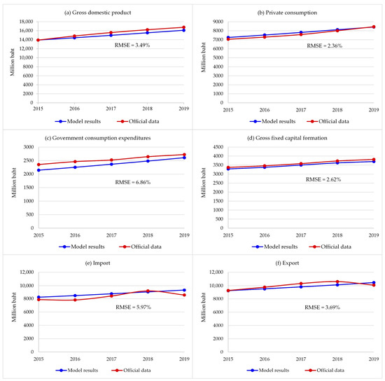
Figure 4.
Discrepancies between model-generated results and official data of the macroeconomic indices for the years 2015–2019.
4.2. Macroeconomic Impacts
4.2.1. Overview of Economic Adjustment
The key macroeconomic indices presented in this study were GDP, consumer price index (CPI), PCON, and GFCF. Table 2 shows a summary of the 10-year average change for each scenario.
Table 2.
Impacts of scenario simulations on macroeconomic indices (% change on average during 2022–2031).
In SIM A, completely removing the biofuel subsidy leads to an economic recession; in this scenario, GDP, PCON, and GFCF decrease by 0.013%, 0.416%, and 0.035%, respectively, whereas CPI increases by 0.171%.
In SIM B, the complete removal of the biofuel subsidy together with 1% TFP enhancement of energy crops leads to better outcomes than SIM A. The GDP is zero which is a higher value than in SIM A (negative), whereas PCON and GFCF are better than in SIM A, with a decrease of 0.403% and 0.029%, respectively. Contrarily, CPI increases by 0.158%, a small degree as compared with SIM A. This implies that enhancing the TFP of energy crops can partially mitigate the negative impacts caused by removing the biofuel subsidy.
In SIM C, a combination of completely removing the subsidy and reallocating 10% of the biofuel subsidy to invest in energy crop plantations is similar to SIM B. The GDP, PCON, and GFCF are reduced by 0.001%, 0.403%, and 0.024%, respectively, whereas CPI increases by 0.155%. This implies that sharing the biofuel subsidy to invest in energy crop plantations can compensate for the loss of economic benefit caused by removing the biofuel subsidy.
Finally, in SIM D, enhancing TFP by 1% and reallocating 10% of the biofuel subsidy to energy crop plantations results in the best economic growth. The GDP rebounds to positive as 0.012%, whereas CPI still increases by 0.143%. PCON and GFCF decrease by 0.390% and 0.018%, respectively. Therefore, the outcomes from this simulation indicate that using TFP improvement and reallocation of the biofuel subsidy for investment in energy crop plantations are optimal policies for mitigating adverse effects.
Figure 5 shows the adjustment of economic agents and firms. In SIM A, the removal of the biofuel subsidy leads to a higher fuel tax on the first path that the government would gain more income. Then, the government has an income for consumption of goods and services. The rest of the government consumption would be transferred for saving, which could be combined with the savings of a household and a foreigner to become the total investment.
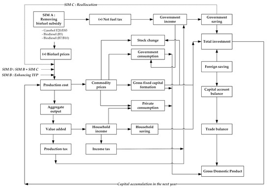
Figure 5.
A flowchart of the economy-wide impacts.
On another path, the removal of biofuel subsidy leads to an increase in biofuel prices. The higher biofuel prices then lead to higher production costs, and commodity prices increase correspondingly, and consequently, the CPI also increases.
Due to higher production costs, the aggregate outputs would decrease, decreasing the value added for all sectors. This situation leads to lower household income and saving. When the household income reduces, the consumption is also eventually decreased. Additionally, the lower household saving also affects government income. The offset between an increase in government saving and a decrease in household saving remains positive for the total investment.
In this study, these three institutes (i.e., household, government, and the world) drive the total investment that is fixed by the closure rule. Given that the government savings increase, the foreign savings would be adjusted to decrease. This implies that removing the biofuel subsidy would indirectly affect a decrease in foreign direct investment. When foreign savings are decreased, it leads to increasing the current account balance and trade balance.
Finally, the GDP change comprises private consumption, government consumption, GFCF, stock changes, and trade balance. In SIM A, the negative impacts of the subsidy removal were similar to findings of previous studies [13,42,43,44,45,46,47].
In SIM B, although the economy endures the negative effects of removing the biofuel subsidy (SIM A), the TFP improvement increases the outputs of energy crop plantations. Therefore, it leads to lower prices of biofuel products and productions; however, removing the biofuel subsidy has a stronger influence than the TFP increment. Therefore, enhancing the TFP of energy crops by 1% could elevate the GDP by 0.013% as compared with SIM A.
Similarly, in SIM C, reallocating the biofuel subsidy to invest 10% in energy crop plantations enhances the GDP by approximately 0.012% as compared with in SIM A. The potential of SIM C is similar to that of SIM B. The investment is to increase capital supply for production sectors. Such an increase leads to the depression of capital costs. Unlike improvement productivity (SIM B), it would increase the quantity of outputs by a larger amount. By comparing SIMs B and C, we can show that a 10% increase in investment is close to a 1% increase in the TFP on energy crops.
In addition, SIM D is a combination between SIMs B and C. This scenario increases the capital supply and efficiency of the energy crop sector. The results indicated that a 1% increase in the TFP and a 10% investment in energy crop plantations can enhance economic growth via a GDP of 0.025% (0.012−(−0.013)) as compared with SIM A.
In summary, the effects of removing the biofuel subsidy could be avoided by enhancing the TFP and reallocating the biofuel subsidy to an investment in energy crop plantations, which are appropriate policies for developing economic and energy production without energy price distortion.
4.2.2. Trends of Macroeconomic Changes
- Gross Domestic Product
Figure 6 shows the trends of the impacts caused by removing biofuel subsidies incorporated with TFP progress and reallocation for investment in energy crop plantations. The results show that removing biofuel subsidies (SIM A) could affect an economic recession because the average GDP decreased by 0.013%; however, the GDP adjustment slowly proceeded until 2031, when the GDP would rebound to be zero. The reason for this is that eliminating biofuel subsidies affects higher biofuel prices and leads to higher production costs. Then, the demand and supply of aggregate outputs also decrease. Therefore, the lower outputs result in a lower GDP; however, the trend of the GDP would be to gradually increase. This increase is in agreement with a previous study [17], which indicated that removing subsidies would enhance the GDP in the long term.
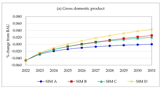
Figure 6.
Projected impacts of four scenarios (SIMs A–D) on gross domestic product during 2022–2031.
To enhance the TFP of energy crops (SIM B), although the average economic growth would be zero, it remains better than SIM A. During 2022–2025, the GDP would be lower than zero, but during 2026–2031, the GDP would rebound to be positive. The two periods, therefore, are offset by each other, because increasing the TFP induces higher total outputs of energy crops and lower production costs. The lower costs of cultivating and harvesting energy crops lead to lower biofuel prices. Given the inverse variation between commodity price and investment demand, lower biofuel prices would lead to higher investment demand for biofuel and continue to trigger capital accumulation in the next year. This process results in increasing the GDP gradually and implies that enhancing the TFP of energy crops could compensate for the negative effects of terminating biofuel subsidies. The results are in line with [37], which stated that improving bioethanol cultivation efficiency enhances economic growth because efficiency would reduce cost per unit and produce more products.
Likewise, reallocating the biofuel subsidy to invest in energy crop plantations (SIM C) affects the average GDP by a decrease of 0.001%, similar to SIM B, because the investments increase the capital of energy crop cultivation. It leads to more production and less unit cost of production in energy crops. When production outputs are increased, the GDP loss is reduced, which indicates that reallocation could also compensate for adverse effects caused by cutting off biofuel subsidies. This simulation result is in line with the finding obtained from an econometrical approach [48].
Finally, if the TFP improvement and investment in energy crop plantations were implemented simultaneously (SIM D), the GDP would recover faster than in SIM B or SIM C. The average GDP growth was positive as 0.012%, because both implementations have double influences on the economy. The TFP would drive productivity, while reallocation would increase the supply of energy crops. Therefore, the GDP would resume to be positive quickly by 2025. Additionally, the average GDP in SIM D is nearly twice that in SIM A.
In summary, all scenarios initially impact GDP loss, but the GDP would gently increase until it becomes positive in the long term. In this case, the best choice is the combination of enhancing TFP and reallocation of biofuel subsidy. The government can completely remove the biofuel subsidy without economic contraction. In the same line of the previous literature [49], these obtained simulation results indicate that the policy reform can lead to the diverse outcomes. The incomplete policy set (SIM A) can incur the negative effect, while the appropriate policy package (SIM D) can influence the sustainable growth path.
- Consumer Price Index
Figure 7 displays the effects of all scenarios on the CPI. In contrast to the GDP, removal of the biofuel subsidy (SIM A) would increase the CPI thoroughly during 2022–2031. Given the higher prices of biofuel, the production sectors would then suffer higher production costs. This result differs from a previous study [18] that reported removal of the oil fund would lead to a decline in the CPI. In this study, at the top level of the production function, as mentioned in Section 3.2, the substitution between primary input and intermediate commodities is assumed to be fixed, and there is no replacement by each other. In addition, mandate and optional biodiesel are subsidized. As a result, there is no choice for people or industry uses, i.e., They must assume there would be higher prices of biodiesel. Unlike gasohol, currently, only gasohol E20 and E85 are still being subsidized. If the subsidies on gasohol E20 and E85 are eliminated, both fuel prices would increase automatically. Instead of using gasohol E20 and E85, people could also switch to use gasohol E10. In reality, biodiesel is a crucial fuel for the transportation and industry sectors. Hence, increasing biodiesel prices caused by terminating subsidies significantly affects the economy.
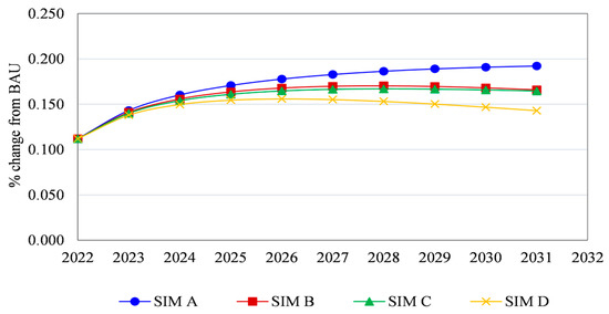
Figure 7.
Projected impacts of four scenarios (SIMs A–D) on consumer price index during 2022–2031.
In contrast, in SIM B, the CPI initially would move up from 2022 to 2028. Afterwards, it would diminish slightly and relatively move as constant. Similarly, the CPIs of both SIMs C and B behave similarly. From 2022 to 2027, the CPI would increase, but from 2027 to 2031, it would be constant. SIM D shows an increase in CPI for only three years (2022–2025), and then it would be stable and decelerate until 2031, because the TFP improvement and investments in energy crop plantations would increase production output and reduce the producer prices of commodities. Therefore, the consumer prices of finished goods would decrease accordingly and promoting the TFP and investment in energy crop plantations by reallocating the biofuel subsidy are appropriate regimes to reduce inflation.
In summary (see Table 2), during such a period, the CPI in SIM A would increase by 0.171% on average, whereas the CPI in SIMs B–D would decrease by 0.158%, 0.155%, and 0.143% on average, respectively.
- Private Consumption
Figure 8 reveals the effects on private consumption, which are similar to the GDP results. The results show that increased biofuel prices resulting from abolishing biofuel subsidies (SIM A) would lead to a decline in the PCON over the period. Initially, the removal of biofuel subsidies would affect the higher production costs and lower outputs and would also lead to lower value added along with a household income reduction. Given the decrease in household income, people must reduce their consumption; therefore, the household would adjust consumption to satisfy budget constraints. The average PCON would decrease by 0.416% (see Table 2).

Figure 8.
Projected impacts of four scenarios (SIMs A–D) on private consumption during 2022–2031.
To enhance the TFP of energy crops (SIM B), although the average PCON decreased by 0.403%, it was still better than in SIM A, because increasing the TFP of energy crops would enhance the total aggregate outputs. Therefore, the household planted energy crops would increasingly earn more income together with consumption. In addition, the higher productivity would affect the increase in outputs of energy crops (e.g., sugar cane, cassava, and oil palm), which are feedstocks of biofuel production. An increase in outputs would lead to a decrease in producer prices through the biofuel supply chain. Then, the commercial biofuel prices would decrease depending on the market mechanism, causing the cost of other production sectors to also decrease. Therefore, the household could consume more than in SIM A; however, enhancing the TFP of energy crops can partially entail adverse effects. The influence of biofuel subsidy removal would be to substantially affect private consumption.
In SIM C, this scenario was to increase the capital supply by reallocating budgets for investment in energy crop plantations. The results showed that the average PCON decreased by 0.403%, equivalent to in SIM B, because the reallocation, in 2022, leads to an increase in capital accumulation, which would result in higher production in the next year. Consequently, the household would gradually receive more income, while the costs of production would inversely decrease. Hence, the PCON and SIM B would increase.
Finally, enhancing the TFP along with investment in energy crop plantations (SIM D) showed that both measures considerably enhanced the PCON growth. Although the average consumption would decline, on average, by 0.390%, the trend would be in an incline direction. The result also displayed an impact almost double that in SIMs B and C. Consequently, this implies that the most appropriate option for maintaining the PCON is TFP improvement and reallocation of budget to invest in energy crop plantations.
- Gross Fixed Capital Formation
Figure 9 demonstrates the changes in the GFCF. The trend of each scenario is different. The oil fund is an organization under government control. Given that biofuel subsidies are cut off, and the government does not need to compensate for biofuel. In SIM A, removing biofuel subsidies could save the oil fund’s liquidation, which would also lead to higher government income and savings. In this study, the total investment is fixed, as mentioned in Section 3.4. The higher prices of commodities caused by increasing production costs would affect the higher values of stock changes. Owing to the inverse variations between the GFCF and stock changes, the GFCF would thus decrease.
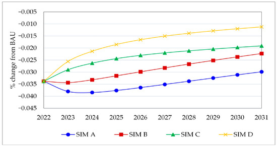
Figure 9.
Projected impacts of four scenarios (SIMs A–D) on gross fixed capital formation during 2022–2031.
In SIM B, the TFP improvement of energy crops leads to an increase in the GFCF, because the lower production costs of energy crops and biofuel products affected lower commodities prices, leading to a decrease in the values of stock changes. Then, the GFCF would increase directly.
In SIM C, the reallocation of budget to invest in energy crop plantations leads to an increase in GFCF. For the same reason as in SIM B, the investment in energy crop plantations increased biofuel feedstocks’ outputs and reduced biofuel prices. Given the decrease in production costs and commodity prices, the values of stock changes would reduce. It would finally lead to an increase in the GFCF. The trend of the GFCF in SIM C was quite different from in SIM B, which implies that reallocating subsidy for investment has more influence on the GFCF than enhancing TFP.
Finally, SIM D combined the TFP with reallocation measures. Although the average GFCF remained less than zero, i.e., 0.018% (see Table 2), the trend increased more than the other scenarios, because of the decrease in commodity prices caused by higher productivity and capital supply of energy crop plantations.
In summary, removing biofuel subsidies vastly affects the GFCF whether using TFP improvement or reallocation of subsidy budget; however, both measures are a desirable choice in the long term because the trends are likely to increase. If policymakers combine both measures to implement energy crops, the adverse effects would be rapidly eliminated more than applying only an individual measure.
4.3. Sectoral Impacts
Table 3 demonstrates the top five impacts on the output of production sectors. Given that the biofuel subsidy was removed, the effects would directly damage the energy and transportation sectors.
Table 3.
Sectoral impacts for SIMs A–D (average during 2022–2031).
In SIM A, the top five sectors, namely ethanol production (cassava-based), coastal and transportation, public road transportation, petroleum refinery, and biodiesel, would decline by 2.874%, 2.396%, 1.800%, 1.722%, and 1.722%, respectively, because a rise in biofuel prices leads to a decrease in biofuel consumption. Therefore, petroleum refineries would decrease production volumes to satisfy domestic demand, and therefore affect the feedstock industry, in particular, ethanol (cassava-based) and biodiesel (B100) productions.
In SIM B, the termination of the subsidy was simultaneously implemented with an increase in energy crop’s cultivation efficiency and induced the substitution between the main feedstocks of ethanol production. Specifically, driven by their different costs, the cassava is used as a substitute for molasses and becomes the main feedstock. Still, in this case, increased prices of fuels reduce transportation activities together with lowering demands for fossil-based fuels and biodiesel.
The simulation results of SIM C show that the policy mix of fuel subsidy removal and a new proportion of energy crop investment yields sectoral impacts similar to those in SIM B. According to the cost gap of ethanol’s feedstocks, this policy mix influences the substitution between cassava and molasses in ethanol production, and simultaneously the productions of petroleum and biodiesel subside.
The outcomes of the last simulation scenario, imposing all combinations of SIMs B and C, indicate that the substitution between ethanol’s feedstocks is the major consequence. Similar to previous simulation results, transportation and petroleum production are negatively affected. Corresponding to the higher biofuel prices and increasing crops’ productivity, the outputs of food-related sectors, which are sugar refinery and crude palm oil, increase. With the higher retail price and the lower transportation demand, biodiesel production still declines as compared with that of the base case.
4.4. Sensitivity Analysis
Figure 10 shows the results obtained from the Monte Carlo simulation. Following the method applied in previous studies [50,51], the coefficients of elasticity of substitution were jointly randomized based on the assumption normal distribution with the standard deviation (SD) of 10% deviation from the original value. The band of two standard deviations (2SD) have been plotted to identify the boundary of the statistical distribution of repeatedly randomized simulations. Similar to the findings of Puttanapong et al. (2015) [52], in the cases of GDP and private consumption, the bands of 2SD will expand over time, implying that these simulated results can be increasingly deviating from the baseline. On the other hand, in the cases of consumer price and gross fixed capital formation, the bands of 2SD will be narrow over the years, indicating that the variation of simulation outcomes will be lower. Hence, in the dynamic dimension, the variation of the coefficients of elasticity of substitution can lead to both cumulative and tapering effects.
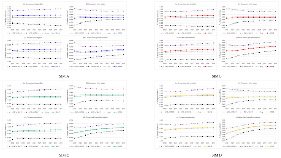
Figure 10.
Statistical distribution of macroeconomic indices.
4.5. Limitations
The limitations of this study are threefold. First, this study used the recursive dynamic mechanism as the main intertemporal process of capital accumulation. This specification can be extended to incorporate the fully dynamic structure incorporating all engonized intertemporal adjustments [31,32]. Second, the knowledge spillover process was arbitrarily assigned in SIM D, but this relationship can be endogenized in the future study [53,54,55]. Third, the model constructed in this study did not include the connection between the adjustment of relative prices and its influence on technical change. This interrelation can be incorporated in the extended version of the existing CGE model [32,56].
5. Conclusions and Recommendations
In this study, we examine the possible combinations of policies to mitigate the impacts of biofuel subsidy removal, develop a reclusive dynamic CGE model, and apply it as the main tool to conduct simulations, revealing the economy-wide propagation mechanisms of impacts and adjustments. We validate the model’s predicted outcomes with actual 2015–2019 data. The obtained values of the RMSE range from 2.62% to 5.97%, affirming the reliability of the model’s predictive power. We simulate four policy scenarios. The first scenario simulation shows that only terminating the biofuel subsidy causes an economy-wide contraction due to causing higher fuel prices. In addition to the subsidy termination, the second and third scenarios incorporate the improvement of energy crop productivity and reallocation of capital investment in energy crop plantations, respectively. The simulation results identify that policy options can mitigate the negative impacts on the Thai economy. The last simulation, which is the combination of the second and third policy options, yields the lowest economy-wide impacts.
These simulation results suggest two recommendations for policymakers. First, termination of the biofuel subsidy along with productivity improvement and reallocation for capital investment in energy crop plantations is the optimal option. Second, substitution between main feedstocks of ethanol production would benefit cassava-based producers and would conversely lower the demand for molasses-based output. Given that the production adjustment requires long-term capital investment, early preparation would mitigate the negative effects on private sectors and consumers.
Author Contributions
Conceptualization, K.P., N.P., and M.P.; data curation, K.P.; formal analysis, K.P.; funding acquisition, M.P.; investigation, K.P. and N.P.; methodology, K.P. and N.P.; project administration, N.P. and M.P.; resource, K.P. and N.P.; software, N.P. and M.P.; supervision, N.P. and M.P.; validation, K.P., N.P., and M.P.; visualization, K.P. and N.P.; writing—original draft preparation, K.P.; writing—review and editing, N.P. and M.P. All authors have read and agreed to the published version of the manuscript.
Funding
This research was funded by the Joint Graduated School of Energy and Environment (JGSEE) and the Sirindhorn International Institute of Technology (SIIT).
Conflicts of Interest
The authors declare no conflict of interest. The funders had no role in the design of the study; in the collection, analyses, or interpretation of data; in the writing of the manuscript, or in the decision to publish the results.
Appendix A
Table A1.
Sectors and commodities in the CGE model
Table A1.
Sectors and commodities in the CGE model
| Sector Number | Industries | IO Code | Commodity Number | Commodities |
|---|---|---|---|---|
| 1 | Agriculture forest and fishery | 001–003, 005–008, 010, 012–029 | 1 | Agriculture forest and fishery |
| 2 | Cassava plantation | 004 | 2 | Cassava |
| 3 | Sugarcane plantation | 009 | 3 | Sugarcane |
| 4 | Oil palm plantation | 011 | 4 | Oil palm |
| 5 | Food industry | 042–054, 056–066 | 5 | Food products |
| 6 | Crude palm oil production | 047 | 6 | Crude palm oil |
| 7 | Sugar refinery | 055 | 7 | Sugar products |
| 8 | Molasses | |||
| 8 | Coal and lignite mining | 030 | 9 | Coal and lignite |
| 9 | Crude oil and natural gas | 031 | 10 | Crude oil and natural gas |
| 10 | Other mining | 032–041 | 11 | Other mineral products |
| 11 | Petroleum refinery | 093–094 | 12 | Liquefied petroleum gas |
| 13 | Jet and kerosene | |||
| 14 | Fuel oil | |||
| 15 | Other petroleum products | |||
| 16 | Gasohol E10 and gasoline | |||
| 17 | Gasohol E20 and E85 | |||
| 18 | Biodiesel B5/7 (mandatory) | |||
| 19 | Biodiesel B10/B20 (option) | |||
| 12 | Biodiesel production | 093 | 20 | Purified biodiesel (B100) |
| 13 | Ethanol (cassava based) | 093 | 21 | Ethanol |
| 14 | Ethanol (molasses based) | 093 | ||
| 15 | Electricity production | 135 | 22 | Electricity |
| 16 | Natural gas separation | 136 | 23 | Natural gas products |
| 17 | Metal and non-metal | 110–111 | 24 | Metal and non-metal |
| 18 | Chemical production | 067–092 | 25 | Chemical products |
| 19 | Rubber and plastic production | 095–109 | 26 | Rubber, plastics, and material |
| 20 | Electrical machinery production | 112–122 | 27 | Electrical machinery and equipment |
| 21 | Transport industry | 123–128 | 28 | Transport machinery and maintenance |
| 22 | Other manufacturing | 129–134 | 29 | Other industrial products |
| 23 | Construction | 137–144 | 30 | Construction |
| 24 | Trading and services | 145–148, 160–164 | 31 | Trading and services |
| 25 | Public administration | 165–171 | 32 | Public administration |
| 26 | Railway freight transportation | 149 | 33 | Railway freight transportation |
| 27 | Railway mass transportation | 149 | 34 | Railway mass transportation |
| 28 | Road public transportation | 150 | 35 | Road public transportation |
| 29 | Road freight transportation (Heavy) | 151 | 36 | Road freight transportation (Heavy) |
| 30 | Road freight transportation (Light) | 151 | 37 | Road freight transportation (Light) |
| 31 | Land transportation services | 152 | 38 | Land transportation services |
| 32 | Ocean and coastal transportation | 153–154 | 39 | Ocean and coastal transportation |
| 33 | Water transportation services | 155 | 40 | Water transportation services |
| 34 | Air transportation | 156 | 41 | Air transportation |
| 35 | Other services and activities | 157–159, 172–180 | 42 | Other services and activities |
Table A2.
Coefficients of elasticity of substitution.
Table A2.
Coefficients of elasticity of substitution.
| Sector Number | Industries | Coefficients of Elasticity of Substitution | ||
|---|---|---|---|---|
| Labor vs. Capital [a] | Biodiesel (B5 vs. B7/B10) [b] | Gasohol (E10 vs. E20/E85) [b] | ||
| 1 | Agriculture forest and fishery | 1.15 | 0.5 | 0.5 |
| 2 | Cassava plantation | 1.15 | 0.5 | 0.5 |
| 3 | Sugarcane plantation | 1.15 | 0.5 | 0.5 |
| 4 | Oil palm plantation | 1.15 | 0.5 | 0.5 |
| 5 | Food industry | 0.86 | 0.5 | 0.5 |
| 6 | Crude palm oil production | 0.86 | 0.5 | 0.5 |
| 7 | Sugar refinery | 0.86 | 0.5 | 0.5 |
| 8 | Coal and lignite mining | 1.1 | 0.5 | 0.5 |
| 9 | Crude oil and natural gas | 1.1 | 0.5 | 0.5 |
| 10 | Other mining | 1.1 | 0.5 | 0.5 |
| 11 | Petroleum refinery | 1.1 | 0.5 | 0.5 |
| 12 | Biodiesel production | 1.1 | 0.5 | 0.5 |
| 13 | Ethanol (cassava based) | 0.86 | 0.5 | 0.5 |
| 14 | Ethanol (molasses based) | 0.86 | 0.5 | 0.5 |
| 15 | Electricity production | 1.02 | 0.5 | 0.5 |
| 16 | Natural gas separation | 1.02 | 0.5 | 0.5 |
| 17 | Metal and non-metal | 0.86 | 0.5 | 0.5 |
| 18 | Chemical production | 0.86 | 0.5 | 0.5 |
| 19 | Rubber and plastic production | 0.86 | 0.5 | 0.5 |
| 20 | Electrical machinery production | 0.86 | 0.5 | 0.5 |
| 21 | Transport industry | 0.87 | 0.5 | 0.5 |
| 22 | Other manufacturing | 0.86 | 0.5 | 0.5 |
| 23 | Construction | 0.97 | 0.5 | 0.5 |
| 24 | Trading and services | 0.87 | 0.5 | 0.5 |
| 25 | Public administration | 1.04 | 0.5 | 0.5 |
| 26 | Railway freight transportation | 1.03 | 0.5 | 0.5 |
| 27 | Railway mass transportation | 1.03 | 0.5 | 0.5 |
| 28 | Road public transportation | 1.03 | 0.5 | 0.5 |
| 29 | Road freight transportation (Heavy) | 1.03 | 0.5 | 0.5 |
| 30 | Road freight transportation (Light) | 1.03 | 0.5 | 0.5 |
| 31 | Land transportation services | 1.03 | 0.5 | 0.5 |
| 32 | Ocean and coastal transportation | 1.03 | 0.5 | 0.5 |
| 33 | Water transportation services | 1.03 | 0.5 | 0.5 |
| 34 | Air transportation | 1.03 | 0.5 | 0.5 |
| 35 | Other services and activities | 1.03 | 0.5 | 0.5 |
Notes: [a] is based on [37]; [b] is based on assumption of authors; For the other types of elasticity i.e., the elasticity of transformation between products of industry j = 2, the elasticity of transformation between exports and local supplies of commodity i by industry j = 2, and the elasticity of substitution between imported and domestically produced commodity i = 2, are based on [24].
Table A3.
Dynamic parameters.
Table A3.
Dynamic parameters.
| Year | n | eg | ig | itg | etr | ppg | δ | γ |
|---|---|---|---|---|---|---|---|---|
| 2019–2031 | 0.01 | 0.05 | 0.05 | 0.055 | 0.05 | 0.01 | 0.07 | 2 |
Notes: n = population growth [33]; eg = government expenditures growth [34]; ig = public sector investment growth [34]; itg = total investment growth [34]; etr = export growth [34]; ppg = total factor productivity growth [35]; δ = depreciation rate [36,37]; γ = elasticity of investment demand [36,37].
References
- Asian Development Bank. Fossil Fuel Subsidies in Thailand: Trends, Impacts, and Reforms; Asian Development Bank: Manila, Philippines, 2015. [Google Scholar]
- Wattana, S. Bioenergy Development in Thailand: Challenges and Strategies. Energy Procedia 2014, 52, 506–515. [Google Scholar] [CrossRef]
- Thai Ethanol Association. Reference Ethanol Prices. Available online: http://www.thai-ethanol.com/th/statistical-data/price.html (accessed on 27 February 2021).
- Department of Alternative Energy Development and Efficiency. Biodiesel Price and Producer Data. Available online: https://www.dede.go.th/more_news.php?cid=88&filename=index (accessed on 27 February 2021).
- Chanthawong, A.; Dhakal, S.; Kuwornu, J.K.M.; Farooq, M.K. Impact of Subsidy and Taxation Related to Biofuels Policies on the Economy of Thailand: A Dynamic CGE Modelling Approach. Waste Biomass Valorization 2020, 11, 909–929. [Google Scholar] [CrossRef]
- United States Department of Agriculture. Thailand Biofuels Annual. Available online: https://apps.fas.usda.gov/newgainapi/api/Report/DownloadReportByFileName?fileName=Biofuels%20Annual_Bangkok_Thailand_11-04-2019 (accessed on 5 February 2021).
- Office of Energy and Policy Planning. Oil Prices. Available online: http://www.eppo.go.th/epposite/index.php/th/petroleum/price/oil-price?category_id=558&isc=0&orders[publishUp]=publishUp&issearch=1 (accessed on 5 February 2021).
- Koesler, S.; Pothen, F. The Basic WIOD CGE Model: A Computable General Equilibrium Model Based on the World Input-Output Database; Zentrum für Europäische Wirtschaftsforschung: Mannheim, Germany, 2013. [Google Scholar]
- Asian Productivity Organization. APO Productivity Databook 2020; Asian Productivity Organization: Tokyo, Japan, 2020. [Google Scholar]
- Warr, P.; Suphannachart, W. Agricultural Productivity Growth and Poverty Reduction: Evidence from Thailand; Departmental Working Papers; The Australian National University, Arndt-Corden Department of Economics: Canberra, Australia, 2020. [Google Scholar]
- Fattouh, B.; El-Katiri, L. Energy Subsidies in the Middle East and North Africa. Energy Strategy Rev. 2013, 2, 108–115. [Google Scholar] [CrossRef]
- Bazilian, M.; Onyeji, I. Fossil Fuel Subsidy Removal and Inadequate Public Power Supply: Implications for Businesses. Energy Policy 2012, 45, 1–5. [Google Scholar] [CrossRef]
- Solaymani, S.; Kari, F. Impacts of Energy Subsidy Reform on the Malaysian Economy and Transportation Sector. Energy Policy 2014, 70, 115–125. [Google Scholar] [CrossRef]
- Breisinger, C.; Engelke, W.; Ecker, O. Leveraging Fuel Subsidy Reform for Transition in Yemen. Sustainability 2012, 4, 2862–2887. [Google Scholar] [CrossRef]
- Lin, B.; Li, A. Impacts of Removing Fossil Fuel Subsidies on China: How Large and How to Mitigate? Energy 2012, 44, 741–749. [Google Scholar] [CrossRef]
- Lin, B.; Jiang, Z. Estimates of Energy Subsidies in China and Impact of Energy Subsidy Reform. Energy Econ. 2011, 33, 273–283. [Google Scholar] [CrossRef]
- Liu, W.; Li, H. Improving Energy Consumption Structure: A Comprehensive Assessment of Fossil Energy Subsidies Reform in China. Energy Policy 2011, 39, 4134–4143. [Google Scholar] [CrossRef]
- Preecha, R.; Wianwiwat, S. The Effect of Abolishing the Oil Fund on the Thai Economy: A Computable General Equilibrium Analysis. Int. Energy J. 2017, 17, 155–162. [Google Scholar]
- Bridle, R.; Sharma, S.; Mostafa, M.; Geddes, A. Fossil Fuel to Clean Energy Subsidy Swaps; International Institute for Sustainable Development: Winnipeg, MB, Canada, 2019. [Google Scholar]
- Castel, V. Economic Brief-Reforming Energy Subsidies in Egypt. Available online: https://www.afdb.org/en/documents/document/economic-brief-reforming-energy-subsidies-in-egypt-26669 (accessed on 13 April 2021).
- Hartono, D.; Komarulzaman, A.; Irawan, T.; Nugroho, A. Phasing out Energy Subsidies to Improve Energy Mix: A Dead End. Energies 2020, 13, 2281. [Google Scholar] [CrossRef]
- Henseler, M.; Maisonnave, H. Low World Oil Prices: A Chance to Reform Fuel Subsidies and Promote Public Transport? A Case Study for South Africa. Transp. Res. Part Policy Pract. 2018, 108, 45–62. [Google Scholar] [CrossRef]
- Farajzadeh, Z.; Bakhshoodeh, M. Economic and Environmental Analyses of Iranian Energy Subsidy Reform Using Computable General Equilibrium (CGE) Model. Energy Sustain. Dev. 2015, 27, 147–154. [Google Scholar] [CrossRef]
- Decaluwe, B.; Lemelin, A.; Maisonnave, H.; Robichaud, V. PEP Standard CGE Models. Available online: https://www.pep-net.org/pep-standard-cge-models (accessed on 17 July 2020).
- Office of the National Economic and Social Development Council. Input-Output Tables (I-O Tables). Available online: https://www.nesdc.go.th/nesdb_en/more_news.php?cid=158&filename=index (accessed on 19 July 2020).
- Department of Alternative Energy Development and Efficiency. Energy Statistics. Available online: https://www.dede.go.th/ewt_news.php?nid=42079 (accessed on 17 May 2020).
- Department of Energy Business, Ministry of Energy. Statistic. Available online: https://www.doeb.go.th/2017/EN_index.html?ln=en#/article/en_statistic (accessed on 10 March 2021).
- Bank of Thailand. Economics Statistics. Available online: https://www.bot.or.th/Thai/Statistics/EconomicAndFinancial/RealSector/Pages/Index.aspx (accessed on 17 May 2020).
- Office of Agricultural Economics. Agricultural Statistics of Thailand 2018. Available online: http://www.oae.go.th/assets/portals/1/files/jounal/2563/yearbook62edit.pdf (accessed on 18 May 2020).
- The Thailand Research Fund E-Library. Available online: https://elibrary.trf.or.th/project_content.asp?PJID=RDG5150022 (accessed on 11 February 2021).
- Bretschger, L.; Ramer, R.; Schwark, F. Growth Effects of Carbon Policies: Applying a Fully Dynamic CGE Model with Heterogeneous Capital. Resour. Energy Econ. 2011, 33, 963–980. [Google Scholar] [CrossRef]
- Bretschger, L.; Zhang, L. Carbon Policy in a High-Growth Economy: The Case of China. Resour. Energy Econ. 2017, 47, 1–19. [Google Scholar] [CrossRef][Green Version]
- Organisation for Economic Co-operation and Development (OECD); International Labor Organization (ILO). How Immigrants Contribute to Thailand’s Economy; OECD Publishing: Paris, France, 2017. [Google Scholar]
- Office of the National Economic and Social Development Council National Income of Thailand. Available online: https://www.nesdc.go.th/nesdb_en/more_news.php?cid=154&filename=index (accessed on 11 February 2021).
- University of Groningen; University of California, Davis Total Factor Productivity at Constant National Prices for Thailand. Available online: https://fred.stlouisfed.org/series/RTFPNATHA632NRUG (accessed on 10 March 2021).
- Annabi, N.; Cockburn, J.; Decaluwe, B. A Sequential Dynamic CGE Model for Poverty Analysis. Available online: http://www.pep-net.org/sites/pep-net.org/files/typo3doc/pdf/files_events/3rd_dakar/SeqDynCGE.pdf. (accessed on 15 March 2021).
- Kaenchan, P.; Puttanapong, N.; Bowonthumrongchai, T.; Limskul, K.; Gheewala, S.H. Macroeconomic Modeling for Assessing Sustainability of Bioethanol Production in Thailand. Energy Policy 2019, 127, 361–373. [Google Scholar] [CrossRef]
- Hosoe, N.; Gasawa, K.; Hashimoto, H. Textbook of Computable General Equilibrium Modeling: Programming and Simulations, 2010th ed.; Palgrave Macmillan: Basingstoke, UK, 2010; ISBN 978-0-230-24814-4. [Google Scholar]
- Suphannachart, W.; Warr, P. Total factor productivity in Thai agriculture: Measurement and determinants. In Productivity Growth in Agriculture: An International Perspective; Fuglie, K.O., Wang, S.L., Ball, V.E., Eds.; CABI: Wallingford, UK, 2012; pp. 215–236. ISBN 978-1-84593-921-2. [Google Scholar]
- Mary, S.; Phimister, E.; Roberts, D.; Santini, F. A Monte Carlo Filtering Application for Systematic Sensitivity Analysis of Computable General Equilibrium Results. Econ. Syst. Res. 2019, 31, 404–422. [Google Scholar] [CrossRef]
- Belgodere, A.; Vellutini, C. Identifying Key Elasticities in a CGE Model: A Monte Carlo Approach. Appl. Econ. Lett. 2011, 18, 1619–1622. [Google Scholar] [CrossRef]
- Acharya, R.H.; Sadath, A.C. Implications of Energy Subsidy Reform in India. Energy Policy 2017, 102, 453–462. [Google Scholar] [CrossRef]
- Moshiri, S.; Martinez Santillan, M.A. The Welfare Effects of Energy Price Changes Due to Energy Market Reform in Mexico. Energy Policy 2018, 113, 663–672. [Google Scholar] [CrossRef]
- Aune, F.R.; Grimsrud, K.; Lindholt, L.; Rosendahl, K.E.; Storrøsten, H.B. Oil Consumption Subsidy Removal in OPEC and Other Non-OECD Countries. Oil Market Impacts and Welfare Effects; Discussion Papers; Statistics Norway, Research Department: Oslo, Norway, 2016. [Google Scholar]
- Bhattacharyya, R.; Ganguly, A. Cross Subsidy Removal in Electricity Pricing in India. Energy Policy 2017, 100, 181–190. [Google Scholar] [CrossRef]
- Wang, Y.; Ali Almazrooei, S.; Kapsalyamova, Z.; Diabat, A.; Tsai, I.-T. Utility Subsidy Reform in Abu Dhabi: A Review and a Computable General Equilibrium Analysis. Renew. Sustain. Energy Rev. 2016, 55, 1352–1362. [Google Scholar] [CrossRef]
- Wesseh, P.K.; Lin, B.; Atsagli, P. Environmental and Welfare Assessment of Fossil-Fuels Subsidies Removal: A Computable General Equilibrium Analysis for Ghana. Energy 2016, 116, 1172–1179. [Google Scholar] [CrossRef]
- AlDarraji, H.H.M.; Bakir, A. The Impact of Renewable Energy Investment on Economic Growth. J. Soc. Sci. COESRJ-JSS 2020, 9, 234–248. [Google Scholar] [CrossRef]
- Karydas, C.; Zhang, L. Green Tax Reform, Endogenous Innovation and the Growth Dividend. J. Environ. Econ. Manag. 2019, 97, 158–181. [Google Scholar] [CrossRef]
- Puttanapong, N. The Computable General Equilibrium (CGE) Models with Monte-Carlo Simulation for Thailand: An Impact Analysis of Baht Appreciation. Ph.D Dissertation, Cornell University, Ithaca, NY, USA, 2008. [Google Scholar]
- Puttanapong, N. Impacts of Climate Change on Major Crop Yield and the Thai Economy: A Nationwide Analysis Using Static and Monte-Carlo Computable General Equilibrium Models. Thail. World Econ. 2013, 31, 68–87. [Google Scholar]
- Puttanapong, N.; Wachirarangsrikul, S.; Phonpho, W.; Raksakulkarn, V. A Monte-Carlo Dynamic CGE Model for the Impact Analysis of Thailand’s Carbon Tax Policies. J. Sustain. Energy Environ. 2015, 6, 43–53. [Google Scholar]
- Aghion, P.; Dechezleprêtre, A.; Hémous, D.; Martin, R.; Van Reenen, J. Carbon Taxes, Path Dependency, and Directed Technical Change: Evidence from the Auto Industry. J. Polit. Econ. 2016, 124, 1–51. [Google Scholar] [CrossRef]
- Calel, R.; Dechezleprêtre, A. Environmental Policy and Directed Technological Change: Evidence from the European Carbon Market. Rev. Econ. Stat. 2016, 98, 173–191. [Google Scholar] [CrossRef]
- Dechezleprêtre, A.; Martin, R.; Mohnen, M. Knowledge Spillovers from Clean and Dirty Technologies; Centre for Climate Change Economics and Policy, London School of Economics and Political Science: London, UK, 2014. [Google Scholar]
- Popp, D. Induced Innovation and Energy Prices. Am. Econ. Rev. 2002, 92, 160–180. [Google Scholar] [CrossRef]
Publisher’s Note: MDPI stays neutral with regard to jurisdictional claims in published maps and institutional affiliations. |
© 2021 by the authors. Licensee MDPI, Basel, Switzerland. This article is an open access article distributed under the terms and conditions of the Creative Commons Attribution (CC BY) license (https://creativecommons.org/licenses/by/4.0/).