Study on the Sensitivity of a Gyroscope System Homing a Quadcopter onto a Moving Ground Target under the Action of External Disturbance

Abstract

This paper investigates the sensitivity (resistance) of a quadcopter on-board gyroscope system for the observation and tracking of a moving ground target to changing parameters of its regulator under interference conditions. It was shown that the gain in matrix elements is most sensitive, and even their slightest deviation from optimal values can lead to reduced target tracking efficiency and even loss of control system stability. Furthermore, the authors studied the energy expenditure at various gyroscope system control parameter values, while homing a quadcopter onto a ground target. A Matlab/Simulink environment was used to conduct simulations of the controlled gyroscope system dynamics. Selected test results are shown in graphic form.

1. Introduction

Currently, one of the most important elements in the equipment of a quadcopter unmanned aerial vehicle (QUAV) is its observation and tracking head. It is used to automatically search and track ground targets, both moving and stationary. Its objective is to determine the position of target line of sight (TLOS) [1,2]. A Gyroscope System (GS) was suggested as a device to control and stabilize TLOS. A relevant issue in terms of such devices is their control under conditions of disturbance induced by the QUAV maneuvering deck.

Previous studies on the dynamics of unmanned aerial vehicles, including a quadcopter, indicated that external disturbance acting on them led to significant errors in the tracking, laser illumination and homing onto both a moving and stationary target [3,4]. In particular, the control system onboard the aforementioned aerial vehicles, did not provide sufficient resistance to vibrations [5,6,7]. A head with controlled gyroscope (its drive) parameters selected optimally for homing precision, should be chosen in order to minimize the aforementioned error.

Such parameters can change in the course of gyroscopic system operation, and the system’s sensitivity to their modification should be tested. This is mainly about determining the scope of change within which the tracking and illumination of a ground target is still sufficiently accurate.

This paper discusses an example of a quadcopter equipped with an EFP (Explosively Formed Projectile) shaped charge that can attack tanks or armored vehicles from the upper ceiling, i.e., from an altitude of several dozen meters, in which an observation and tracking head scans the surface of the Earth from onboard the drone, searching for an object emitting infrared radiation. Upon detecting a target, the QUAV enters the self-homing phase using the proportional navigation method. The target can be simultaneously illuminated with a laser beam enabling it to be attacked, with other external means of precise striking (antitank missile or a bomb homing onto a reflected laser beam). It is also possible for an ultralight drone to land directly on a tank in order to emit signals that can be intercepted by the heads of other means of attack, e.g., rocket missiles on ground launchers or fixed under the wings of flying vehicles (helicopters, aircraft or unmanned aerial vehicles).

In the source literature, there are many examples of the widespread use of drones in various areas of today’s life, such as in [8,9]. It should be noted that the proposed system in this paper differs significantly from the above-mentioned works and the those discussed in [10,11], mainly due to the use of an original gyro guidance head. Also, many algorithms and onboard systems have already been developed for quadcopter stabilization and motion control. Most of them use sensors to measure the position of the copter, such as gyroscopes, accelerometers or IMU/MEMS units [12,13] but lack information on conducted studies involving the use of a mechatronic controller gyroscope onboard a quadcopter. It should be stressed that one of the major advantages of such a gyroscope is its resistance to vibrations and random interference, including noise. Furthermore, the authors propose gyroscope system controls, optimal in terms of precision and energy expenditure, ensuring the most stable and effective homing of the drone onto a target.

The parts of this publication have been organized as follows: Section 2 discusses a method for the determination of optimal parameters for the controlled GS. Section 3 includes the results of an analysis covering the simulation tests of the gyroscope system sensitivity to changing its regulator parameters under the conditions of interference, when illuminating a ground target with a QUAV onboard laser. It also contains the results of simulation tests regarding GS control energy expenditure within the process of homing a quadcopter onto a moving ground target. Section 4 summarizes the study and presents the final conclusions.

2. Determining Optimal Parameters for a Controlled Gyroscope System

A linearized model of a controlled gyroscope system is expressed in the following form [14,15,16]:

$$\frac{d{\mathit{x}}_g}{dt}={\mathit{A}}_g{\mathit{x}}_g-{\mathit{B}}_g{\mathit{u}}_g,$$

(1)

where:

• ${\mathit{x}}_g={\left[\begin{array}{cccc}{\vartheta }_g& {\dot{\vartheta }}_g& {\psi }_g& {\dot{\psi }}_g\end{array}\right]}^T$—state vector, ${\mathit{u}}_g={\left[\begin{array}{cc}{M}_b& M_c\end{array}\right]}^T$—control vector,
• ${\mathit{A}}_g=\left[\begin{array}{cccc}0& 1& 0& 0\\ 0& -b_b& 0& -1\\ 0& 0& 0& 1\\ 0& 1& 0& -b_c\end{array}\right]$—state matrix, ${\mathit{B}}_g=\left[\begin{array}{cc}0& 0\\ c_b& 0\\ 0& 0\\ 0& c_c\end{array}\right]$—control matrix,
• $b_b=\frac{{\eta }_b}{J_{gk}\Omega }$, $b_c=\frac{{\eta }_c}{J_{gk}\Omega }$, $c_b=c_c=\frac{1}{J_{gk}{\Omega }^2}$, $\Omega =\frac{J_{go}{n}_g}{J_{gk}}$,
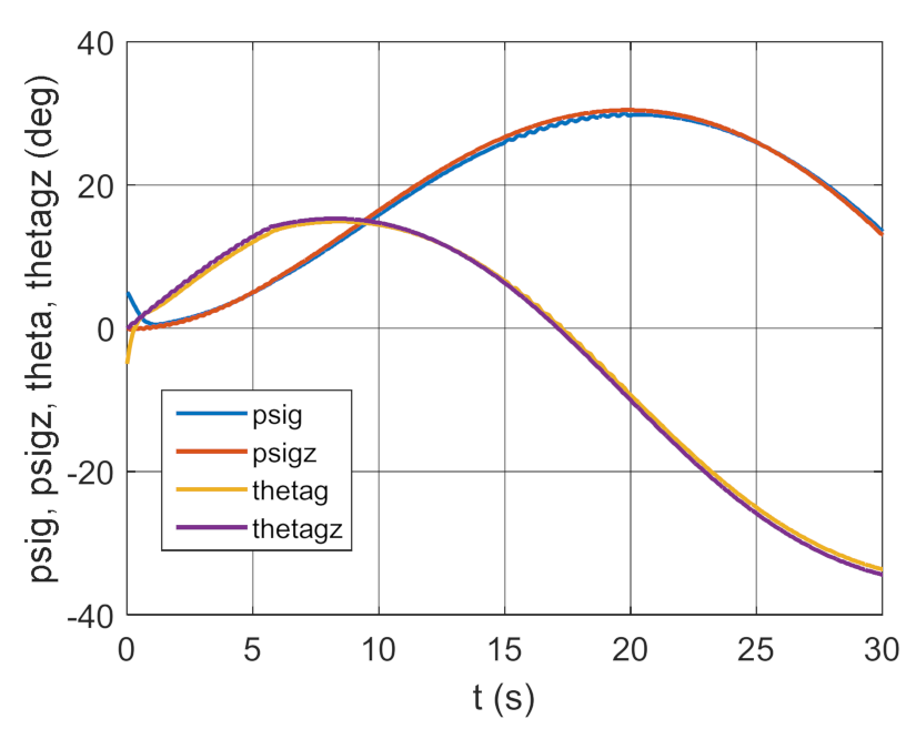
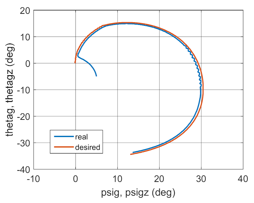
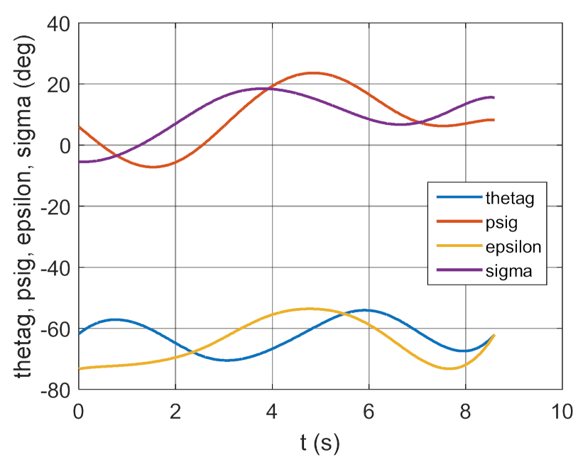
• ${\vartheta }_g, {\psi }_g$—angles defining the position of the GS axis in space,
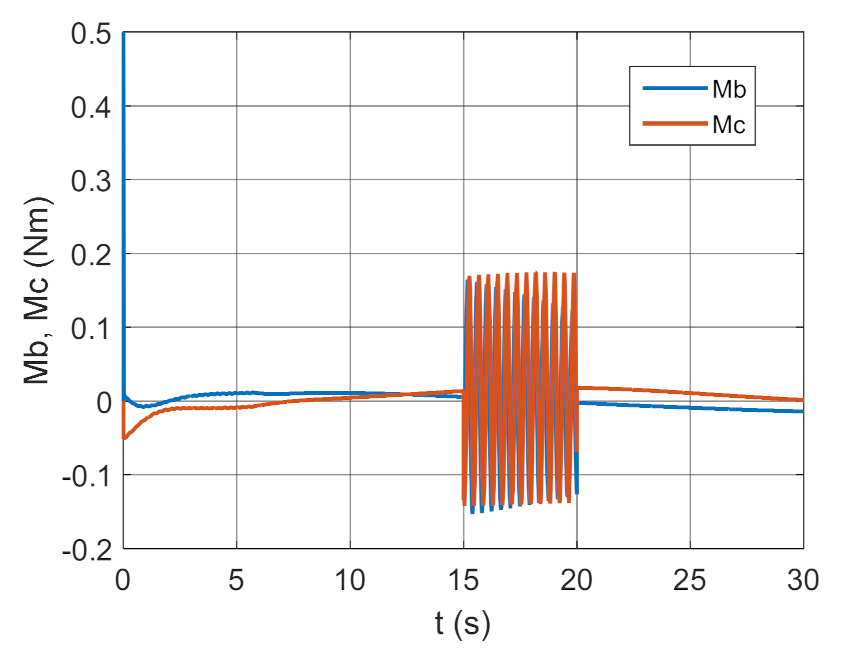
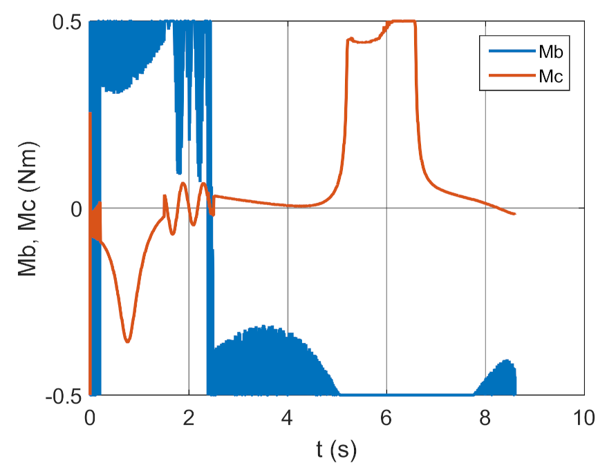
• $M_b, M_c$—control moments,
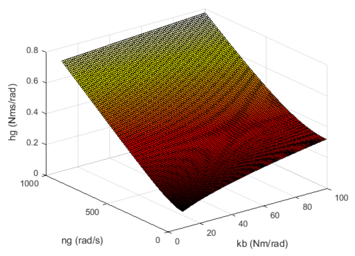
• ${\eta }_b, {\mathsf{\eta }}_c$—damping coefficients in GS frame suspension bearings,
• $J_{go}$—moment of inertia of a GS rotor relative to the longitudinal axis,
• $J_{gk}$—moment of inertia of a GS rotor relative to the transverse axis,
• $n_g$—rotary speed of the GS rotor.

In order to provide the controlled gyroscope, described by Equation (1), with the stability and shortest decay time of transition to a set value, let us introduce optimal control in the form:

$${\mathit{u}}_g=-{\mathit{K}}_g{\mathit{x}}_g,$$

(2)

where:

${\mathit{K}}_g=\left[\begin{array}{cccc}{k}_{11}& k_{12}& k_{13}& k_{14}\\ k_{21}& k_{22}& k_{23}& k_{24}\end{array}\right]$—gain matrix.

After taking into account the above assumptions using the LQR method and analytical solution of the Riccati equation, individual elements of the gain matrix ${\mathit{K}}_g$ for the analysed gyroscope system satisfy the following relationship [14]:

$$k_{11}=k_{23}={\overline{k}}_b, k_{12}=k_{14}=k_{22}=k_{24}={\overline{h}}_g, k_{21}=-k_{13}={\overline{k}}_c.$$

(3)

After substituting gain coefficient (3) to (2), correction controls will be expressed in the following form:

$$M_b=-k_b{\overline{\vartheta }}_g+{\overline{k}}_c{\psi }_g-{\overline{h}}_g\frac{d{\vartheta }_g}{dt},$$

(4)

$$M_c=-k_c{\overline{\vartheta }}_g-{\overline{k}}_b{\psi }_g-{\overline{h}}_g\frac{d{\psi }_g}{dt},$$

(5)

where:

$${\overline{k}}_b=\frac{k_b}{J_{gk}{\mathsf{\Omega }}^2}, {\overline{k}}_c=\frac{k_c}{J_{gk}{\mathsf{\Omega }}^2}, {\overline{h}}_g=\frac{h_g}{J_{gk}\mathsf{\Omega }}.$$

(6)

Therefore, the open-system gyroscope system (1), taking into account (4), i.e., after substituting $M_b$ and $M_c$ in the control vector ${\mathit{u}}_g$, is reduced to a new form (closed-system):

$$\frac{d{\mathit{x}}_g}{dt}={\mathit{A}}_g^{*}{\mathit{x}}_g,$$

(7)

where:

$${\mathit{A}}_g^{*}=\left[\begin{array}{cccc}0& 1& 0& 0\\ -{\overline{k}}_b& -{\overline{h}}_g-b_b& +{\overline{k}}_c& 1\\ 0& 0& 0& 1\\ -{\overline{k}}_c& -1& -{\overline{k}}_b& -{\overline{h}}_g-b_c\end{array}\right].$$

Further, let us assume that friction in the gyroscope suspension bearings is negligible i.e., $b_b=b_c=0$. For such a described gyroscope system, let us additionally look for such parameters and inter-relations, which guarantee the shortest transient process damping time. In this case let us also use a modified method of the Golubientsev optimization method, which consists in ensuring the fastest disappearance of transient processes that appear after switching on the control, or a sudden operation of a disturbance. The algorithm of this method is presented in [14].

Using the Hurwitz stability criterion and the modified Golubientsev optimization method [14,17], we obtain the following system of equations and inequalities:

$${\overline{k}}_b>0, {\overline{k}}_c>0, {\overline{h}}_g>0,$$

(8)

$$2{\overline{k}}_b-\frac{1}{2}{\overline{h}}_g^2+1>0,$$

(9)

$${\overline{k}}_c=\frac{1}{2}{\overline{h}}_g,$$

(10)

$$\frac{1}{16}{\overline{h}}_g^4+\frac{1}{4}{\overline{h}}_g^2-\frac{1}{2}{\overline{h}}_g^2{\overline{k}}_b-{\overline{h}}_g{\overline{k}}_c+{\overline{k}}_b^2+{\overline{k}}_c^2>0.$$

(11)

Taking into account the maximization condition for the absolute trace value of matrix ${\mathit{A}}_g^{*}$

$$\left|Tr{\mathit{A}}_g^{*}\right|\to max,$$

(12)

Using inequality (9) we obtain the following value of the damping coefficient:

$${\overline{h}}_g=\sqrt{2+4{\overline{k}}_b}.$$

(13)

Substituting (13) to the Equation (10) we get:

$${\overline{k}}_c=\frac{1}{2}\sqrt{2+4{\overline{k}}_b}.$$

(14)

Whereas, after taking into account (6) we get:

$$h_g=\sqrt{2J_{go}^2{n}_g^2+4J_{gk}{k}_b },$$

(15)

$$k_c=\frac{1}{2}\frac{J_{go}^2{n}_g^2}{J_{gk}}\sqrt{2J_{go}^2{n}_g^2+4J_{gk}{k}_b}.$$

(16)

Thus, coefficients ${\overline{h}}_g$ and ${\overline{k}}_c$ are explicitly defined as the gyroscope parameter functions $J_{go},J_{gk}$ and $n_g$ of the coefficient ${\overline{k}}_b$, which should satisfy the stability criteria as well as the technical restrictions arising from the strength of the gyroscope structure itself.

The obtained relationships can be used for controlling the gyroscope under conditions of changing specific rotation angular velocity (e.g., in certain drones with a limited and unstable power source). In such a case, one should measure the $n_g\left(t\right)$ values on an ongoing basis and updated the ${\overline{h}}_g$ and ${\overline{k}}_c$ regulator coefficient values in accordance with the relationships (15) and (16). Coefficient ${\overline{k}}_b$ is set through software. This enables adaptive gyroscope control. The adaptive control algorithm described in [14] should be used for cases of numerous other parameters of the gyroscope changing over time. Figure 1 and Figure 2 graphically characterize the relationships between individual parameters of the gyroscope and its regulator. In order to obtain the aforementioned relationships, it was assumed that $J_{gk}=J_{go}/2$.

Figure 1. Graph of optimal inter-relations between the regulator damping coefficient $h_g$, angular velocity $n_g$ and the gain coefficient $k_b$.

Figure 2. Graph of optimal inter-relations between the regulator gain coefficient $k_c$, angular velocity $n_g$ and the gain coefficient $k_b$.

Therefore, if the system of terms (8)–(11) is satisfied, the gyroscope system transient process induced by external disturbance (1) is damped first.

3. Test Results

This section presents the results and analysis of the tests covering the dynamics of the controlled gyroscope system with the following parameters [2,18]:

$$J_{x_1}=2.5·{10}^{-5}{ \mathrm{kgm}}^2, J_{y_1}=J_{x_1}, J_{z_1}=J_{x_1},$$

$$J_{x_2}=5·{10}^{-5}{ \mathrm{kgm}}^2, J_{y_2}=J_{x_2}, J_{z_2}=J_{x_2},$$

$$J_{x_3}=J_{go}=5·{10}^{-4}{ \mathrm{kgm}}^2, J_{y_3}=J_{gk}=2.5·{10}^{-4}{ \mathrm{kgm}}^2,$$

$$J_{z_3}=J_{x_3}, m_2=0.1 \mathrm{kg}, m_3=0.14 \mathrm{kg}, m_g=m_2+m_3,$$

$$n_g=600 \mathrm{rad}/\mathrm{s}; {\eta }_b={\eta }_c=0.05 \mathrm{Nm}/\mathrm{s}.$$

The kinematic excitations acting on the gyroscope system were assumed to be harmonic forms with an amplitude equal to $0.5 \mathrm{rad}/\mathrm{s}$ and frequency equal to $15 \mathrm{rad}/\mathrm{s}$.

The simulation testing was conducted in the Matlab/Simulink environment (Version R2020a, MathWorks, Natick, MA, USA), with an integration step of $dt=0.00001 \mathrm{s}$ [19].

3.1. Test Results Regarding the Sensitivity of a Gyroscope System during Tracking and Laser Illumination of a Ground Target

Let us assume that the initial conditions do not match set conditions:

$${\psi }_{go}\ne {\psi }_{gzo}, {\vartheta }_{go}\ne {\vartheta }_{gzo}, {\dot{\psi }}_{go}\ne {\dot{\psi }}_{gzo}, {\dot{\vartheta }}_{go}\ne {\dot{\vartheta }}_{gzo},$$

and are equal:

$${\psi }_{go}=5 \mathrm{deg}, {\vartheta }_{go}=-5 \mathrm{deg}, {\dot{\psi }}_{go}=0, {\dot{\vartheta }}_{go}=0.$$

Control moments were adopted in the following form:

$$M_b=-k_b{e}_{\vartheta }+k_c{e}_{\psi }-h_g{\dot{e}}_{\vartheta }, M_c=-k_c{e}_{\vartheta }-k_b{e}_{\psi }-h_g{\dot{e}}_{\psi },$$

where:

$$e_{\vartheta }={\vartheta }_g-{\vartheta }_{gz}, {\dot{e}}_{\vartheta }={\dot{\vartheta }}_g-{\dot{\vartheta }}_{gz}, e_{\psi }={\psi }_g-{\psi }_{gz}, {\dot{e}}_{\psi }={\dot{\psi }}_g-{\dot{\psi }}_{gz}.$$

It was also assumed that the task of gyroscope system control was displacement over a minimum time and maintaining the gyroscope axis in a position consistent with the target line of sight position, with an error below 0.5 degrees, i.e., 0.0087 rad. After satisfying this condition, it activates only the laser system to illuminate the target. The target should be steadily illuminated, with preset precision, regardless of the drone maneuvers, vibrations of its deck and other external disturbances, such as wind gusts [20,21] or projectile explosion. Such disturbances appeared within the simulation in question, in the period between 15 to 20 s.

Figure 3, Figure 4, Figure 5 and Figure 6 contain simulation results for nonoptimal regulator coefficients:

$$k_b=10, k_c=100, h_g=100.$$

Figure 3. Real and set angle of gyroscope system (GS) deflection and inclination as a function of time.

Figure 4. Real and desired motion trajectory.

Figure 5. Control moments as a function of time.

Figure 6. Total error as a function of time.

The simulation results presented in Figure 3, Figure 4, Figure 5 and Figure 6 clearly show that the controller parameters are chosen incorrectly. There are significant deviations of the actual values of the position angles of the GS axis ${\psi }_g, {\vartheta }_{g }$ from the pre-set values ${\psi }_{gz}, {\vartheta }_{gz }$ (Figure 3 and Figure 4). Consequently, the control error reaches large values (Figure 6). The kinematic excitations occurring after 15 s of motion have a very negative effect on the motion of the gyroscope system, which can also be seen in Figure 5.

Figure 7, Figure 8, Figure 9 and Figure 10 show simulation results for other nonoptimal values of regulator coefficients of

$$k_b=10, k_c=10, h_g=10.$$

Figure 7. Real and set angle of GS deflection and inclination as a function of time.

Figure 8. Real and desired motion trajectory.

Figure 9. Control moments as a function of time.

Figure 10. Total error as a function of time.

From the simulation results shown in Figure 7, Figure 8, Figure 9 and Figure 10, it can be seen that the motion of the gyroscope system is more stable. The deviations from the set values are smaller than for the case shown in Figure 3, Figure 4, Figure 5 and Figure 6. However, the control error is still too large, whereas Figure 11, Figure 12, Figure 13 and Figure 14 contain test results for a regulator coefficient of $k_b=10$, while $k_c$ and $h_g$ are determined based on relationships (13)–(14) (i.e., optimal).

Figure 11. Real and set angle of GS deflection and inclination as a function of time.

Figure 12. Real and desired motion trajectory.

Figure 13. Control moments as a function of time.

Figure 14. Total error as a function of time.

The results presented in Figure 11, Figure 12, Figure 13 and Figure 14 show that the controller with the optimal parameters work properly. The trajectory of the actual motion almost coincides with the desired trajectory. The total control error for the steady-state motion oscillates around a value equal to 1 degree.

Figure 15, Figure 16, Figure 17 and Figure 18 shows the test results for optimal regulator coefficients of $k_b=348$ and $k_c$ and $h_g$ determined based on relationships (13)–(14).

Figure 15. Real and set angle of GS deflection and inclination as a function of time.

Figure 16. Real and desired motion trajectory.

Figure 17. Control moments as a function of time.

Figure 18. Total error as a function of time.

Such a selection of control coefficients causes the changes over time of the actual angles of GS axis position and the set angles to coincide almost perfectly, which can also be seen in Figure 16. The influence of kinematic excitations on GS motion is imperceptible. The total control error is close to zero.

Some selected test results shown in Figure 3, Figure 4, Figure 5, Figure 6, Figure 7, Figure 8, Figure 9, Figure 10, Figure 11, Figure 12, Figure 13, Figure 14, Figure 15, Figure 16, Figure 17 and Figure 18 indicate that the most important regulator parameter is the k_b coefficient, which was ultimately selected so that the control moments did not exceed the permissible absolute values of 0.5 Nm on one hand, and the total error between the set and implemented gyroscope axis position was below 0.5 degrees (0.0087 rad) on the other. Other coefficients were determined based on the relationships (7)–(15). Numerous tests involving gyroscope system sensitivity indicated that with an optimally selected k_b coefficients, other coefficients, namely $k_c$ and $h_g$, varying within 30% of the optimum values, did not cause significant errors in maintaining the gyroscope axis in accordance with the target line of sight. Errors exceeding permissible values, i.e., axis deviation from the set value higher than 0.0087 rad appeared after leaving the aforementioned change range of the coefficients. At the same time, the control moments reached unacceptable values.

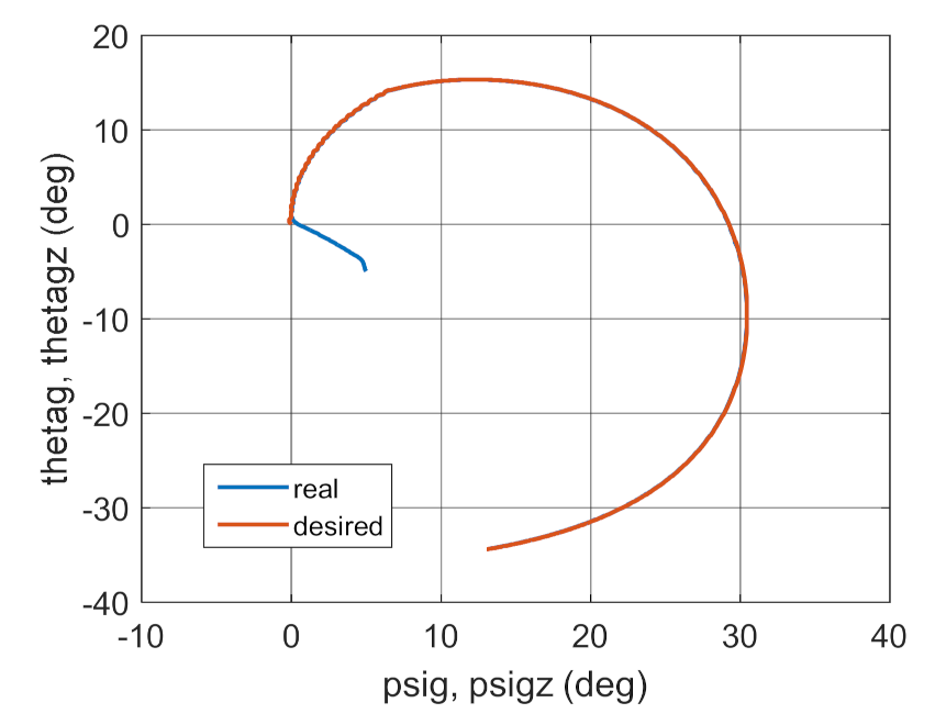
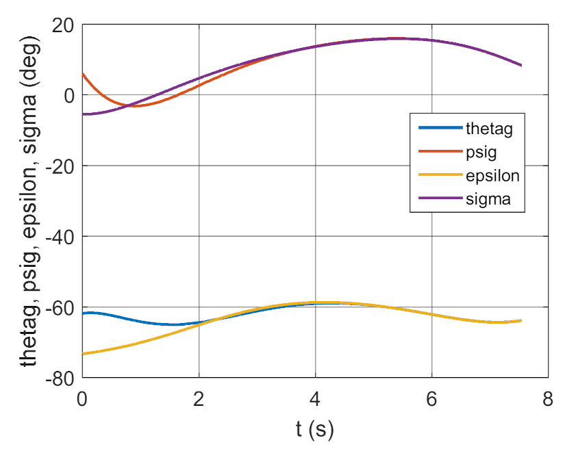
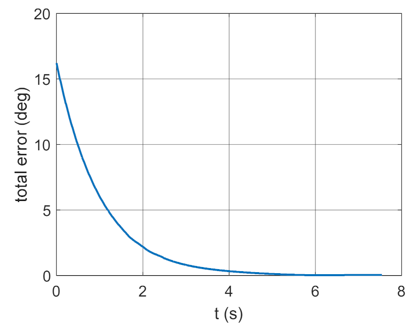
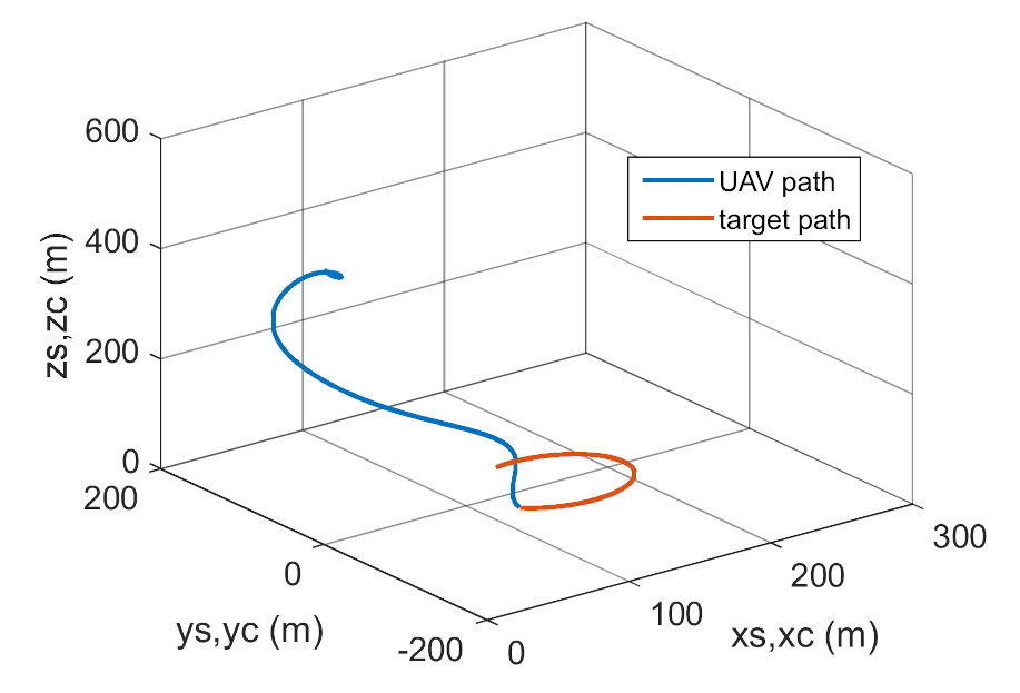
3.2. Simulation Studies Involving the Control over an Optimum Gyroscope System for Homing onto a Ground Target from Onboard a Quadcopter

In order to test the operating effectiveness of a gyroscope system with optimally selected parameters when homing a quadcopter onto a moving ground target under conditions of external disturbance, the following controls, quality indicators and initial conditions of drone and target motion were adopted.

GS axis control moments:

$$M_b=-k_b{e}_{\vartheta }+k_c{e}_{\psi }-h_g{\dot{e}}_{\vartheta }, M_c=-k_c{e}_{\vartheta }-k_b{e}_{\psi }-h_g{\dot{e}}_{\psi }$$

where:

$$e_{\vartheta }={\vartheta }_g-\epsilon ; {\dot{e}}_{\vartheta }={\dot{\vartheta }}_g-\dot{\epsilon }; e_{\psi }={\psi }_g-\sigma ; {\dot{e}}_{\psi }={\dot{\psi }}_g-\dot{\sigma }$$

$\epsilon , \sigma$—deflection and inclination angles of the target line of sight, determined from homing kinematics equations.

In terms of selecting the optimum parameters for the gyroscope system in question, the following two quality indicators were adopted:

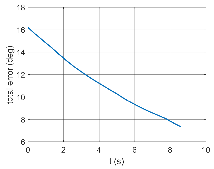
• IAE (Integral Absolute Error) quality indicator:

  $$\mathrm{IAE}=\underset{0}{\overset{\infty }{{\displaystyle \int }}}\left|e_c\right|dt$$

  where:

$e_c=\sqrt{e_{\vartheta }^2+e_{\psi }^2}$—total error.

2.

ISSC (Integral Square State and Control) quality indicator:

$$\mathrm{ISSC}=\underset{0}{\overset{\infty }{{\displaystyle \int }}}\left(x^{T}x\right)dt+\underset{0}{\overset{\infty }{{\displaystyle \int }}}\left(u^{T}u\right)dt$$

where:

$$x=\left[\begin{array}{cccc}{\vartheta }_g& {\psi }_g& {\dot{\vartheta }}_g& {\dot{\psi }}_g\end{array}\right], u=\left[\begin{array}{cc}{M}_b& M_c\end{array}\right].$$

Initial positions and angular velocities of gyroscope system axis position:

$${\psi }_g=\sigma +0.2 \mathrm{rad}, {\vartheta }_g=\epsilon +0.2 \mathrm{rad}, {\dot{\psi }}_g=0; {\dot{\vartheta }}_g=0.$$

Initial ground target movement conditions:

$$x_c=150 \mathrm{m},y_c=50 \mathrm{m},z_c=0.$$

$$V_c=25 \mathrm{m}/\mathrm{s}, {\gamma }_c=0, {\chi }_c=0.$$

Initial drone flight parameters:

$$x_s=0, y_s=0, z_s=500 \mathrm{m}.$$

$$V_s=75\frac{\mathrm{m}}{\mathrm{s}}, {\gamma }_s=\epsilon , {\chi }_s=\sigma .$$

Coefficient $k_b$ is selected heuristically, while the optimum PD regulator gain coefficients is calculated from relationships (13)–(14).

The analysis involved six variants with two GS control parameter values.

The test results shown in Figure 19, Figure 20, Figure 21, Figure 22, Figure 23, Figure 24, Figure 25, Figure 26, Figure 27, Figure 28, Figure 29, Figure 30, Figure 31, Figure 32, Figure 33, Figure 34, Figure 35, Figure 36, Figure 37, Figure 38, Figure 39, Figure 40, Figure 41, Figure 42, Figure 43, Figure 44, Figure 45, Figure 46, Figure 47 and Figure 48 and determined quality indicator values in Table 1 indicate that effective control over a gyroscope system when homing a quadcopter onto a moving ground target under external disturbance conditions requires the application of optimum regulator parameters, with values from a range determined based on the tests discussed in Section 3.1.

Table 1. Quality indicators.

Variant	Regulator Parameters	ISSC	IAE
1	$k_b=10, k_c=10, h_g=10$	9.2403 × 108	5.3726 × 103
2	$k_b=10, k_c=100, h_g=100$	9.6861 × 108	7.2331 × 103
3	$k_b=10, k_c, h_g$ − optimum	1.1070 × 109	4.3352 × 103
4	$k_b=348, k_c, h_g$ − optimum	1.6691 × 109	1.7290 × 103
5	$k_b=348, k_c, h_g=0.7\ast \mathrm{optimum}$	1.6845 × 109	1.8137 × 103
6	$k_b=348, k_c,h_g=1.3\ast \mathrm{optimum}$	1.6263 × 109	1.9237 × 103

The tests also indicated that with an optimally selected coefficient $k_b$, the values of coefficients $k_c$ and $h_g$ can change over a broad range but cannot exceed 30% of the optimum values. Figure 36 and Figure 46 clearly show that a gyroscope system in variant 6 was faster in “entering” the set trajectory but the IAE indicator reached a much higher value relative to variant 4, with comparable values of the ISSC indicator for both variants.

A similar situation applies to variant 5. The value of coefficients $k_c$ and $h_g$ were 30% lower than the optimum values, which significantly increased the gyroscope system homing error. This is particularly visible when comparing Figure 36 and Figure 41.

In conclusion, it should be stated that the assumed homing accuracy is achieved for optimum gyroscope control system regulator values adopted in variant 4.

Variant 1.

$$k_b=10;k_c=10;h_g=10.$$

Figure 19. Trajectories of unmanned aerial vehicle (UAV) and target flight.

Figure 20. Changes of realizing and pre-set deflection and inclination angles of GS as a time function.

Figure 21. Trajectories of the real and desired motion.

Figure 22. Control moments as a function of time.

Figure 23. Total error as a function of time.

Variant 2.

$$k_b=10;k_c=100;h_g=100.$$

Figure 24. Trajectories of UAV and target flight.

Figure 25. Changes of realizing and pre-set deflection and inclination angles of GS as a time function.

Figure 26. Trajectories of the real and desired motion.

Figure 27. Control moments as a function of time.

Figure 28. Total error as a function of time.

Variant 3.

$k_b=10$, whereas $k_c, h_g$ are adopted optimum values.

Figure 29. Trajectories of UAV and target flight.

Figure 30. Changes of realizing and pre-set deflection and inclination angles of GS as a time function.

Figure 31. Trajectories of the real and desired motion.

Figure 32. Control moments as a function of time.

Figure 33. Total error as a function of time.

Variant 4.

$k_b=348$, whereas $k_c, h_g$ adopted optimum values.

Figure 34. Trajectories of UAV and target flight.

Figure 35. Changes of realizing and preset deflection and inclination angles of GS as a time function.

Figure 36. Trajectories of the real and desired motion.

Figure 37. Control moments as a function of time.

Figure 38. Total error as a function of time.

Variant 5.

$k_b=348$, whereas $k_c, h_g$ are adopted values 30% lower than optimum.

Figure 39. Trajectories of UAV and target flight.

Figure 40. Changes of realizing and pre-set deflection and inclination angles of GS as a time function.

Figure 41. Trajectories of the real and desired motion.

Figure 42. Control moments as a function of time.

Figure 43. Total error as a function of time.

Variant 6.

$k_b=348$, whereas $k_c, h_g$ are adopted values 30% higher than optimum.

Figure 44. Trajectories of UAV and target flight.

Figure 45. Changes of realizing and preset deflection and inclination angles of GS as a time function.

Figure 46. Trajectories of the real and desired motion.

Figure 47. Control moments as a function of time.

Figure 48. Total error as a function of time.

Table 1 shows the values of determined quality indicators.

The data presented in Table 1 show that the IAE indicator is the decisive criterion for the selection of regulator parameters. The ISSC does not give unambiguous answers. The lowest value of the IAE indicator was achieved for variant 4. The parameters of the regulator determined in this variant made it possible to obtain the highest accuracy of guiding the quadcopter to the moving target.

4. Conclusions

The optimum parameters for controlling the gyroscope axis position presented herein minimize the error between the set and desired movements to acceptable values and reduce the impact of kinematic excitation of the QUAV base and external disturbance acting on the drone. The authors studied sensitivity and determined the optimum parameter change ranges for stable, precise tracking, laser illumination and homing onto a moving ground target from onboard a drone.

Due to a minimum offset between the set and implemented gyroscope axis position, a specific optimum coefficient k_b was determined for the controlled gyroscope system in question. The GS is very sensitive to changes in this coefficient. Other coefficients, $k_c$ and $h_g$, are functions of $k_b$ and the GS is not really sensitive to changes in their values, since they can vary by up to 30% of optimum values without a significant impact on the precision of ground target tracking and laser illumination.

Summing up, it can be concluded that the application of a gyroscope system with optimally selected parameters ensures stable and precise QUAV homing onto a moving ground target under external disturbance.

The next stage of the research will be the application of the optimal parameters set out in this paper for the experimental verification of the operation of the gyro system guiding the quadcopter onto a moving ground target to prove ground conditions.

References

- Gapinski, D.; Krzysztofik, I. The process of tracking an air target by the designed scanning and tracking seeker. In Proceedings of the 2014 15th International Carpathian Control Conference (ICCC), Velke Karlovice, Czech Republic, 28–30 May 2014; IEEE: New York, NY, USA; pp. 129–134. [Google Scholar] [CrossRef]
- Stefański, K.; Koruba, Z. Analysis of the guiding of bombs on ground targets using a gyroscope system. J. Theor. Appl. Mech. 2012, 50, 967–973. [Google Scholar]
- Chodnicki, M.; Bartnik, K.; Nowakowski, M.; Kowaleczko, G. Design and analysis of a feedback loop to regulate the basic parameters of the unmanned aircraft. Aircr. Eng. Aerosp. Technol. 2018, 92, 318–328. [Google Scholar] [CrossRef]
- Kowaleczko, G.; Pietraszek, M.; Słonkiewicz, Ł. Analysis of the Impact of the Target Illumination Time on the Effectiveness of the Flight Trajectory Correction System. J. Konbin 2019, 49, 229–253. [Google Scholar] [CrossRef]
- Hasseni, S.; Abdou, L. Decentralized PID Control by Using GA Optimization Applied to a Quadrotor. J. Autom. Mob. Robot. Intell. Syst. 2018, 12, 33–44. [Google Scholar] [CrossRef]
- Praveen, V.; Pillai, A.S. Modeling and simulation of quadcopter using PID controller. Int. J. Control Theory Appl. 2016, 9, 7151–7158. [Google Scholar]
- Zulu, A.; John, S. A Review of Control Algorithms for Autonomous Quadrotors. Open J. Appl. Sci. 2014, 4, 547–556. [Google Scholar] [CrossRef]
- Xuan-Mung, N.; Hong, S.K. Robust Backstepping Trajectory Tracking Control of a Quadrotor with Input Saturation via Extended State Observer. Appl. Sci. 2019, 9, 5184. [Google Scholar] [CrossRef]
- Xuan-Mung, N.; Hong, S.K.; Nguyen, N.P.; Ha, L.N.N.T.; Le, T.-L. Autonomous Quadcopter Precision Landing Onto a Heaving Platform: New Method and Experiment. IEEE Access 2020, 8, 167192–167202. [Google Scholar] [CrossRef]
- Xuan-Mung, N.; Hong, S.-K. Improved Altitude Control Algorithm for Quadcopter Unmanned Aerial Vehicles. Appl. Sci. 2019, 9, 2122. [Google Scholar] [CrossRef]
- Xuan-Mung, N.; Hong, S.-K. A Multicopter Ground Testbed for the Evaluation of Attitude and Position Controller. Int. J. End. Technol. 2018, 7, 65–73. [Google Scholar]
- Shi, X.; Lu, L.; Jin, G.; Tan, L. Research on the attitude of small UAV based on MEMS devices. AIP Conf. Proc. 2017, 1839, 020094. [Google Scholar] [CrossRef]
- Kumar, P.; Praveen, B.; Nisanth, U.; Hemanth, M. Development of Auto Stabilization Algorithm for UAV Using Gyro Sensor. Int. J. Eng. Res. Technol. 2017, 5, 1–3. [Google Scholar]
- Awrejcewicz, J.; Koruba, Z. Classical Mechanics. Applied Mechanics and Mechatronics; Springer: New York, NY, USA, 2012; Volume 30. [Google Scholar]
- Lewis, F.L.; Vrabie, D.L.; Syrmos, V.L. Optimal Control; John Wiley & Sons: Hoboken, NJ, USA, 2012. [Google Scholar]
- Tewari, A. Modern Control Design with Matlab and Simulink; John Wiley & Sons: Chichester, UK, 2002. [Google Scholar]
- Kaczorek, T.; Dzieliński, A.; Dąbrowski, W.; Łopatka, R. Fundamentals of Control Theory; WNT: Warsaw, Poland, 2013. [Google Scholar]
- Krzysztofik, I.; Takosoglu, J.; Koruba, Z. Selected methods of control of the scanning and tracking gyroscope system mounted on a combat vehicle. Annu. Rev. Control 2017, 44, 173–182. [Google Scholar] [CrossRef]
- Baranowski, L. Effect of the mathematical model and integration step on the accuracy of the results of computation of artillery projectile flight parameters. Bull. Pol. Acad. Sci. Tech. Sci. 2013, 61, 475–484. [Google Scholar] [CrossRef][Green Version]
- Grzyb, M.; Stefanski, K. Turbulence impact on the control of guided bomb unit. In Proceedings of the 23rd International Conference Engineering Mechanics 2017, Svratka, Czech Republic, 15–18 May 2017; Brno University of Technology: Brno, Czech Republic; pp. 358–361. [Google Scholar]
- Kowaleczko, G.; Żyluk, A. Influence of atmospheric turbulence on bomb release. J. Theor. Appl. Mech. 2009, 47, 69–90. [Google Scholar]
Publisher’s Note: MDPI stays neutral with regard to jurisdictional claims in published maps and institutional affiliations. |
© 2021 by the authors. Licensee MDPI, Basel, Switzerland. This article is an open access article distributed under the terms and conditions of the Creative Commons Attribution (CC BY) license (http://creativecommons.org/licenses/by/4.0/).