A Perturbation-Based Methodology to Estimate the Equivalent Inertia of an Area Monitored by PMUs

Abstract

This paper proposes a novel methodology to estimate equivalent inertia of an area, observed from its boundary buses where Phasor Measurement Units (PMUs) are assumed to be installed. The areas are divided according to the measurement points, and the methodology proposed can obtain the equivalent dynamic response of the area dependent of or independent of coherency of the generators inside, which is the first contribution of this paper. The methodology is divided in three parts: estimating the frequency response, estimating the power imbalance and estimating inertia through the solution of the swing equation by Least-Squares Method (LSM). The estimation of the power imbalance is the second contribution of this paper, enabling the study of areas that contain perturbations and attending the limitation of methods of the literature that rely on assumptions of slow mechanical power. It can be further divided in three steps: accounting the total power injected, estimating an equivalent load behavior and estimating an equivalent mechanical power. The quality of results is proved with test systems of different sizes, simulating different types of perturbations.

1. Introduction

The increasing penetration of Renewable Energy Sources (RES) in power systems is bringing new challenges to Transmission System Operators (TSOs) worldwide. RES-based generators are connected to the grid by means of converters that electrically decouple their inertial response, if any, from the system. Hence, equivalent inertia is decreasing, causing higher and faster frequency excursions following power imbalances, which may result in frequency instability. To mitigate this impact, a requirement of synthetic compensation of inertia is being adopted by many TSOs [1,2]. However, RES are intermittent, such that assessing equivalent inertia is a rising need [3,4].

A possibility to estimate equivalent inertia is provided by the recently deployed and disseminated PMUs, devices capable of providing measurements of frequency, current and voltage (magnitude and phase angles) in real time in a precise and synchronized way, with a resolution of 10–60 samples per second [5]. Due to the easiness of working with phasors, PMUs have been used in many different applications, such as analysis of perturbations and oscillations [6,7,8], topology monitoring and parameter estimation [9]. Regarding inertia estimation, literature normally divides the topic in small perturbation studies [8,10,11], large perturbation studies [12,13,14] and studies under ambient conditions [15,16].

In the field of large perturbation studies, a particular effort has been devoted in recent years to characterize areas including multiple loads and generators. However, most papers assume either monitoring generating units individually or monitoring coherent groups of generators. In [17], a robust Kalman Filter is proposed to estimate the mean frequency, but full dynamical observability is required. In [18], an approach that accommodates frequency and voltage variations through curve-fitting is proposed, but accuracy highly depend on the percentage of generating units monitored. In [19], the inertia of an area as perceived by a particular bus of the system is evaluated through an autoregressive moving average exogenous input model, but in all testes, generators are assumed as monitored.

However, monitoring generating units individually may be hard to ensure in real systems. Despite recent efforts on developing low-cost solutions [20,21,22], most commercial PMUs are still expensive [23,24], such that most countries still count with a limited number of PMUs installed. Hence, difficulties for TSOs are many: not all generators individually monitored, coherent groups always changing due to the impact of intermittent RES-based generation, lack of observability of medium-voltage and low-voltage grids, and limited or slow communication.

Taking these practical aspects into consideration, this paper proposes a novel way of looking at the problem: instead of defining an area through the traditional criteria of coherency adopted in the literature, an area may be defined according to the location of available PMUs in the network. Whether considering units already installed or planning the placement of new PMUs, the proposed requirements to define an area based on phasor measurements are just two: to monitor the total power injected by the area in the system, and to monitor the dynamics of the Center of Inertia (COI) of the area. Whenever these requirements are met, an area can be defined, and a dynamic equivalent can be obtained.

The methodology proposed can build a dynamic equivalent of an area in three major steps: estimating the frequency response, estimating the power imbalance and estimating inertia. To estimate the frequency response, the methodology reduces the system around the measurement points available and adapts part of the method proposed in [25] to obtain equivalents at the retained points. The many equivalents are then combined in one, which represents the dynamics of the COI of the area. To estimate power imbalance of the area, the methodology proposes estimating the behavior of the total load, total losses and total mechanical power of the area, seen from its boundary buses. Finally, inertia is estimated solving the swing equation related to the dynamic equivalent of the area through LSM.

Results are obtained with data provided by simulations with the well-known 11-bus Kundur’s test system [26] and with the benchmark test system proposed in [27]. The first part of the results section presents a study validating the methodology, with details about its steps and insights on the behavior of the dynamic equivalents. A switch of a synchronous generator by a Wind Power (WP) generator is simulated, and the reduction of inertia following the event is estimated with the methodology proposed. The second part of the results section presents different study cases evaluating the performance of each step and its impact on the final inertia estimated.

Thus, the main contribution of this paper is the innovative manner of defining areas based on practical assumptions. Second, the methodology derived is capable of estimating inertia regardless the coherency of generators inside the area of study. Finally, the methodology can deal with perturbations inside or outside the area considered.

The remaining of this paper is organized as follows: Section 2 presents a brief introduction on the dynamic behavior of an area, Section 3 presents the methodology, Section 4 presents the results and Section 5 presents the conclusions.

2. The Dynamic Behavior of an Area

The dynamics of a synchronous machine i following a perturbation is ruled by the Swing Equation,

$$\frac{2H_i}{2\pi f_0}\frac{d^2{\delta }_i\left(t\right)}{d{t}^2}=\Delta P_i\left(t\right)=P_{m_i}\left(t\right)-P_{g_i}\left(t\right),\left[pu\right]$$

(1)

where $H_i$ is the constant of inertia, ${\delta }_i$ is the rotor angle, $\Delta P_i\left(t\right)$ is the total power imbalance, $P_{m_i}$ is the mechanical power and $P_{g_i}$ is the electrical power produced by machine i. Additionally, the term $\frac{d^2{\delta }_i\left(t\right)}{d{t}^2}$ may be changed to $\frac{d{f}_i\left(t\right)}{dt}$ since

$$f_i=\frac{1}{2\pi }\frac{d{\delta }_i\left(t\right)}{dt}+f_0,\left[Hz\right]$$

(2)

where $f_0$ is the nominal frequency of the system.

To evaluate the dynamic behavior of a multi-machine system, it is possible to write Equation (1) for every machine that is connected to the grid. Alternatively, it is also possible to study the behavior of the system with an equivalent, based on the concept of the COI, a rotational analogy of the center of mass of an object. The dynamic behavior of every synchronous generator tends to follow the behavior of the COI of the system [26]. This concept may be particularized to any group of generators, restricted to a regional area of interest, for example. The restriction of the area of study is a matter of deciding the extension of the data set [10].

The frequency associated with the COI (also called mean frequency), is a weighted average of the frequencies of every machine of the area, determined by

$$f_{CO{I}_a}\left(t\right)=\frac{{\sum }_{i=1}^n{H}_i{S}_{b_{Gi}}{f}_{G_i}\left(t\right)}{{\sum }_{i=1}^n{H}_i{S}_{b_{Gi}}}$$

(3)

where $H_i$ is the inertia, $S_{b_{Gi}}$ is the nominal power and $f_{G_i}$ is the electrical frequency of each generator $G_i$ in Area a.

The constant of inertia at the COI of Area a is

$$H_{CO{I}_a}=\sum _{i=1}^n{H}_i{S}_{b_{Gi}}$$

(4)

Furthermore, the dynamic behavior of an area may be studied from the point of view of its boundary bus (or boundary buses). Consider the left part of Figure 1 as a generic representation of an area of a power system. An equivalent of Area a seen from its boundary bus (BB) is represented in the right part of the figure, where $M_a$ represents the moving masses of the area, $P_{mo{v}_a}$ is the moving power, $G_{e{q}_a}$ is an equivalent generator and $P_{e_a}$ is the power exiting the area. To represent $G_{e{q}_a}$, the second-order model is assumed in Figure 1, where $x_a^{\prime }$ is the transient reactance and ${\mathbf{E}}_a$ is the internal voltage of the machine.

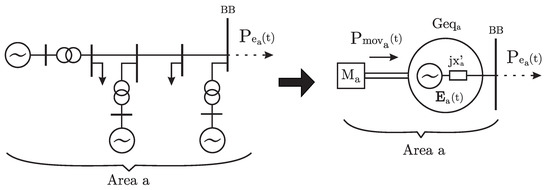
Figure 1. Equivalent system of an area seen from its boundary bus.

The moving power of Area a is defined here as:

$$P_{mo{v}_a}\left(t\right)\triangleq P_{m_a}\left(t\right)-P_{l_a}\left(t\right)-P_{losse{s}_a}\left(t\right)\triangleq \sum _{i=1}^n{P}_{m_i}\left(t\right)-\sum _{l=1}^{n_l}{P}_{l_l}-\sum _{m=1}^{n_b}{P}_{losse{s}_m}$$

(5)

where $P_{m_a}$ denotes the total mechanical power, $P_{l_a}$ denotes the total load power and $P_{losse{s}_a}$ denotes the total losses of area a; $P_{m_i}$ denotes the mechanical power of each of the $i=1,$ …$,n$ generators, $P_{l_l}$ denotes the active power consumed at each of the $l=1,$ …$,n_l$ load buses and $P_{losse{s}_m}$ are the losses in each of the $m=1,$ …$,n_b$ branches inside the area a.

The Swing Equation that rules the dynamics of the equivalent system can be written as

$$\frac{H_{CO{I}_a}}{\pi f^0}\frac{d^2{\delta }_a\left(t\right)}{d{t}^2}=\Delta P_a\left(t\right)=P_{mo{v}_a}\left(t\right)-P_{e_a}\left(t\right),p.u.$$

(6)

where $H_a$ is the overall inertia of the dynamic equivalent, ${\delta }_a$ is the phase angle of the internal voltage ${\mathbf{E}}_a$, $\Delta P_a\left(t\right)$ is the total power imbalance of Area a and $P_{e_a}\left(t\right)$ is the total power injection at BB. The phase angle ${\delta }_a$ may be considered to be an approximation of the mean rotor angle ${\varphi }_a$ according to

$${\varphi }_a\left(t\right)=\frac{{\sum }_{i=1}^n{H}_i{S}_{b_{Gi}}{\varphi }_{G_i}\left(t\right)}{{\sum }_{i=1}^n{H}_i{S}_{b_{Gi}}}$$

(7)

where ${\varphi }_{G_k}\left(t\right)$ is the rotor angle of each generator $i=1$ … n of area a, and the other variables have been previously defined following Equation (3).

3. Methodology

In the technical literature, the definition of equivalent circuit of areas takes place according to coherency criteria, such that generators behaving similarly may be easily grouped together. This proposition has been widely adopted because it facilitates system reduction, diminishing computational effort in dynamic simulations. Here, instead, the aim is not system reduction for simulations, but system reduction for parameter estimation and system dynamic assessment. Therefore, a new way of defining an area is here adopted, based on the location of PMUs in the grid.

To define an area for the study, two requirements need to be fulfilled: the total power injected by the area and the dynamics of its COI must be monitored/estimated. If this is true, it is possible study the dynamics of the area with an equivalent, following the theory in Section 2. Therefore, a methodology is derived in this paper with the aim of modelling the dynamic behavior of an area through the equivalent Equation (6). To do so, ${\delta }_a\left(t\right)$, $P_{mo{v}_a}\left(t\right)$ and $P_{e_a}\left(t\right)$ have to be monitored or estimated, and $H_{CO{I}_a}$ is obtained as an outcome of the procedure.

Consider an Area a monitored by PMUs installed at its BBs (PMU-1 and PMU-2) and at possible buses inside (PMU-N), as represented in Stage 1 of Figure 2, where dotted lines represent the many connections inside the area. The first step of the methodology consists of reducing the system around the n measurement points, as shown in Stage 2 of Figure 2. Assuming that the interconnections of the system do not change during the period of study, the power exported by Area a through its boundary buses (measured) may be assumed as $P_{e_a}\left(t\right)$ in Equation (6).

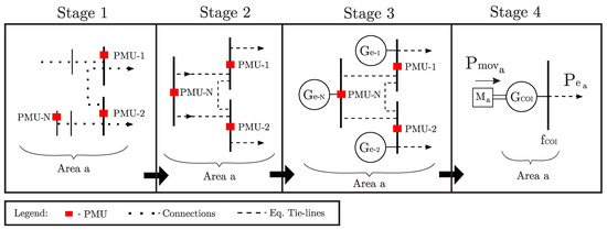
Figure 2. PMU-based system reduction.

The dynamics of the hidden machines inside the reduced area are approximated through the estimation of equivalent generators at the points retained (Stage 3 of Figure 2). After the equivalent generators are obtained, it is possible to calculate their mean dynamic behavior (i.e., ${\delta }_a\left(t\right)$) to feed Equation (6). This procedure is described in detail in Section 3.1.

The dynamic behavior of the n equivalent generators above mentioned may be represented together by the COI of the area, as represented in Stage 4. Most methods available in the literature for inertia estimation following perturbations require monitoring the terminal buses where generators are connected, and rely on the assumption that the mechanical power changes slowly in comparison to the electrical power generated by the machine [25,28,29]. However, when monitoring an area through its boundaries, this assumption becomes too strict: due to load behavior and possible perturbations inside the area, the moving power may not behave slow in comparison to the electrical power injected. In this condition, the equivalent moving power of Area a must also be estimated to estimate $H_{CO{I}_a}$ accurately. This procedure is described in Section 3.2.

After ${\delta }_a\left(t\right)$, $P_{mo{v}_a}\left(t\right)$ and $P_{e_a}\left(t\right)$ are obtained, Equation (6) can be used to estimate $H_{CO{I}_a}$. This is approached in Section 3.3.

At the end of the section, Section 3.4 presents a flowchart summarizing the full methodology.

3.1. Determination of the COI Dynamics

Starting from Stage 1 of Figure 2, the first step is to reduce the system around the measurement points available. System reduction methods were first developed in the literature for speeding up calculations and simulators [30]. Consequently, some of the criteria to reduce the system may not be reasonable for the goal of this paper, as they were tailored for model simulation, but some techniques may be adopted. The Ward Equivalent method is a generalization of the Thévenin equivalent, widely used with phasorial representation in steady-state studies, that can be extended to represent part of grid in quasi-static conditions.

Assuming the loads modelled as constant impedance, the steady-state operation point and the network topology in this context as known, it is possible to retain the buses where PMUs are available, eliminating the others, as in Stage 2 of Figure 2. At this point, the dynamic of the hidden generators is not yet represented (they will be represented together in the equivalents obtained in Stage 3).

The system reduction starts from the full algebraic equations, which are valid for each time step $t=1,\cdots ,M$ when considering the transient evolving under quasi-static conditions and small frequency variations. By Ohm’s law,

$${\mathbf{Y}}_{BUS}{\mathbf{V}}_{Bt}={\mathbf{I}}_{Bt}$$

(8)

where ${\mathbf{Y}}_{BUS}$ is the admittance matrix of the system (built not including generator and load admittances), with dimensions $N_T\times N_T$, where $N_T$ is the total number of buses in the system. The vectors ${\mathbf{V}}_{Bt}$ and ${\mathbf{I}}_{Bt}$ are respectively the bus voltages and current injections vectors at time step t, with dimensions $N_T\times 1$.

The current injection at a generic bus b${\mathbf{I}}_{B_t}^{\left(b\right)}$ can be written as:

$${\mathbf{I}}_{B_t}^{\left(b\right)}={\mathbf{I}}_{G_t}^{\left(b\right)}-{\mathbf{I}}_{L_t}^{\left(b\right)}$$

(9)

where ${\mathbf{I}}_{G_t}^{\left(b\right)}$ is the generator current of bus b, ${\mathbf{I}}_{L_t}^{\left(b\right)}$ is the load current and ${\mathbf{I}}_{B_t}^{\left(b\right)}$ is the injected current in the grid and the superscript denote bus b.

Defining the buses where PMUs are installed as the set of buses to be retained ($R=\{1,2,\cdots ,N\}$), then ($N_T-N$) buses must be eliminated ($E=b\notin R$).

Equation (8) can be reorganized as:

$$\left[\begin{array}{cc}{\mathbf{Y}}_{RR}& {\mathbf{Y}}_{RE}\\ {\mathbf{Y}}_{ER}& {\mathbf{Y}}_{EE}\end{array}\right]\left[\begin{array}{c}{\mathbf{V}}_R\\ {\mathbf{V}}_E\end{array}\right]=\left[\begin{array}{c}{\mathbf{I}}_R\\ {\mathbf{I}}_E\end{array}\right]$$

(10)

where the subscripts R and E are related to the retained and eliminated buses, respectively. For the sake of simplicity, the subscript t is neglected here.

Equation (10) may be manipulated to obtain

$$({\mathbf{Y}}_{RR}-{\mathbf{Y}}_{RE}{\mathbf{Y}}_{EE}^{-1}{\mathbf{Y}}_{ER}){\mathbf{V}}_R={\mathbf{I}}_R-{\mathbf{Y}}_{RE}{\mathbf{Y}}_{EE}^{-1}{\mathbf{I}}_E$$

(11)

Making

$${\mathbf{Y}}_{EQ}={\mathbf{Y}}_{RR}-{\mathbf{Y}}_{RE}{\mathbf{Y}}_{EE}^{-1}{\mathbf{Y}}_{ER}$$

(12)

and

$${\mathbf{I}}_W=-{\mathbf{Y}}_{RE}{\mathbf{Y}}_{EE}^{-1}{\mathbf{I}}_E$$

(13)

it is possible to rewrite Equation (11) as

$${\mathbf{Y}}_{EQ}{\mathbf{V}}_R={\mathbf{I}}_{R_{EQ}}$$

(14)

It is important to observe that ${\mathbf{I}}_{R_{EQ}}$ in Equation (14) can be obtained with the voltage phasors at the retained buses ${\mathbf{V}}_R$ and the reduced admittance matrix ${\mathbf{Y}}_{EQ}$, therefore practical conditions.

With ${\mathbf{I}}_{EQ}$ and ${\mathbf{V}}_R$, it is possible to apply a model estimation method at each retained bus to obtain the equivalent generators represented in Stage 3 of Figure 2. The method proposed in [25] requires current and voltage measurements at the terminals of a generator to estimate its second-order model. Here, the method is applied in another context: building dynamic equivalents from the voltages and currents obtained at the retained buses (${\mathbf{I}}_{EQ}$ and ${\mathbf{V}}_R$), which may be generation buses (originally) or not.

At each retained bus, one equivalent generator will be obtained. In general terms, this is done relating the assumptions of a second-order model and the power injected in the grid at the connection point, as shown in Figure 3. In the figure, Bus k is a retained bus, $P_{e_k}$ is the power injected and $Ge{q}_k$ is the equivalent generator, whose parameters are estimated from ${\mathbf{V}}_k\left(t\right)$ and ${\mathbf{I}}_k\left(t\right)$, the terms of the matrices ${\mathbf{V}}_R$ and ${\mathbf{I}}_{EQ}$ related to Bus k, respectively. As fast as $Ge{q}_k$ concerned, it is needed to estimate the transient reactance $x_k^{\prime }$ and the internal voltage ${\mathbf{E}}_k$; $M_k$ is the moving mass and $P_{mo{v}_k}\left(t\right)$ is the moving power.

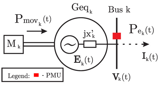
Figure 3. Equivalent generator estimated from the retained bus k.

Assuming that the magnitude of ${\mathbf{E}}_k$ is constant (which is an intrinsic assumption of the second-order model), the method fits Kirchhoff’s equations with input signals to estimate first an equivalent transient reactance $x_k^{\prime }$; in fact, the following equation holds,

$$E_k\left(t\right)\angle {\delta }_k\left(t\right)=\left(j{x}_k^{\prime }\right)I_k\left(t\right)\angle {\alpha }_k\left(t\right)+V_k\left(t\right)\angle {\theta }_k\left(t\right)$$

(15)

Since $E_k$ is constant, it is possible to assume the variance $Var$ equal to zero

$$Var\left(E_k\right)\approx 0$$

(16)

From Equation (15),

$$|{\mathbf{E}}_{\mathbf{k}}\left(t\right)|=\sqrt{{x_k^{\prime }}^2|{\mathbf{I}}_k{\left(t\right)|}^2+{\left|{\mathbf{V}}_k\left(t\right)\right|}^2+2x_k^{\prime }{Q}_k\left(t\right)}$$

(17)

and

$$E_k{\left(t\right)}^2={x_k^{\prime }}^2{I}_k{\left(t\right)}^2+V_k{\left(t\right)}^2+2x_k^{\prime }{Q}_k\left(t\right)$$

(18)

where $Q_k\left(t\right)$ is the reactive power injection at Bus k that can be calculated from ${\mathbf{V}}_k\left(t\right)$ and ${\mathbf{I}}_k\left(t\right)$.

Based on Equation (16), it is possible to write

$$Var\left(E_k^2\right)\approx 0\to \overline{{(E_k^2-\overline{E_k^2})}^2}\approx 0$$

(19)

where $\overline{E}=mean\left(E\right)$.

Fitting (18) into (19) results in

$$({x_k^{\prime }}^2{I}_k^2+V_k^2+2x_k^{\prime }{Q}_k)-({x_k^{\prime }}^2\overline{I_k^2}+\overline{V_k^2}+2x_k^{\prime }\overline{Q_k})\approx 0$$

(20)

Rearranging Equation (20) and assuming measurements at every time step t, holds:

$${x_k^{\prime }}^2(\overline{I_{k_t}^2}-I_{k_t}^2)+x_k^{\prime }\left(2(\overline{Q_{k_t}}-Q_{k_t})\right)\approx (V_{k_t}^2-\overline{V_{k_t}^2})$$

(21)

Expression (21) can be solved for $x_k^{\prime }$ using a nonlinear LSM. In the present work, the trust-region-reflective method is chosen [31].

After $x_k^{\prime }$ is calculated, it is possible to come back to Equation (15) and calculate $E_k\angle {\delta }_k\left(t\right)$.

At this point, it is possible to obtain an estimation of ${\varphi }_a\left(t\right)$ based on ${\delta }_k\left(t\right)$, adapting Equation (7). As $S_{bGi}$ and $H_i$ are unknown, it is possible to assume weights for the equivalent generators obtained in the previous passages of the methodology. These weights may be adjusted to privilege the equivalents obtained from data collected close to big generation centers or close to the possible physical location of the COI, for example. Therefore, in this context,

$${\delta }_a^{est}\left(t\right)=\frac{{\sum }_{k=1}^n{W}_k{\delta }_{G_k}}{{\sum }_{k=1}^n{W}_k}$$

(22)

where the superscript est denotes estimation and $W_k$ is the weight adopted to each equivalent $k=1$ … n. Please note that Equation (22) provides an approximation of the mean rotor angle of Area a based on the rotor angles of the N equivalent generators obtained at the buses where PMUs are installed (which might be generation buses or not). Equation (22), instead, is based on the n generators inside Area a.

3.2. Determination of the Equivalent Moving Power

As defined in Equation (5), $P_{mo{v}_i}\left(t\right)$ is composed by the contributions of the mechanical power ($P_m$) of the machines inside the area, the contributions of loads ($P_l$) and the contributions of losses ($P_{losses}$). The methodology approaches $P_l$ first, assuming a model for the loads and estimating the total contribution according to measurements available. This step is described in Section 3.2.1. With $P_l$ and the power injected into the area ($P_e$), it is possible to estimate the total power generated $P_g$, assuming a typical rate for $P_{losses}$ during the procedure. This step is described in Section 3.2.2. Finally, $P_m$ is estimated through model identification, in the procedure described in Section 3.2.3.

3.2.1. Estimation of the Dynamic Behavior of the Loads

Many different papers discuss the use of PMUs for monitoring, studying or estimating load behavior. In [32] the use of a PMU to monitor and estimate the behavior of induction motors is addressed, detailing practical limitations. Papers [33,34] propose different approaches for dynamic load modelling in distribution grids. In [35], a practical approach based on modelling the load as constant current is presented. The methodology assumes the total load pre-disturbance as known, and by weighting voltage measurements at different buses it can estimate the equivalent load behavior of an area. Papers [36,37], instead, are model-identification-based. They make use of optimization for estimating the parameters of the ZIP model [37] or exponential voltage/frequency dependence model [36].

The fields of load estimation and load characterization is wide and have their own challenges. According to the model chosen to characterize the load, different methods are available. A complex method is both requiring in terms of observability and time consuming. In this work, load estimation is only an auxiliary method necessary for a further goal that is inertia estimation: hence, a simple approach that keeps practical conditions is used. According to [38], the voltage dependence of the loads has a more significant impact on the power imbalance and on inertia estimation studies than frequency dependence. Therefore, a static load model was chosen in this work.

In the constant impedance model, the total power consumed by all loads of an area can be expressed by

$$P_l\left(t\right)=P_{ref}\sum _{i=1}^{nl}\frac{V_{l_i}^2\left(t\right)}{V_{l_{i0}}^2}$$

(23)

where $P_{ref}$ is a reference value of the total load of the area; $V_{l_{i0}}$ is the initial voltage magnitude at bus i; $V_{l_i\left(t\right)}$ is the magnitude of voltage at bus i at time t and $nl$ is the number of load buses.

When applying Equation (23), $P_l\left(t\right)$ varies according to the variations in $V_{l_i}^2\left(t\right)$ if the perturbation is not directly on the loads of the system. If the perturbation is a load step or disconnection, $P_{ref}$ should change to reflect that, but the problem is that in general, that perturbation is neither known nor measured directly. Here, such change in $P_{ref}$ is estimated as follows

$$\begin{array}{cc}\hfill & P_{ref}\left(t\right)=P_{L_{total}}^{st1},fort<t_e\hfill \\ \hfill & P_{ref}\left(t\right)=P_{L_{total}}^{st2},fort\ge t_e\hfill \end{array}$$

(24)

where $P_{L_{total}}$ is the average value of the total load of the area at the steady-state before $\left(st1\right)$ and after the perturbation $\left(st2\right)$, and $t_e$ is the time of occurrence of the event. In this paper, $P_{L_{total}}$ is assumed as known and $t_e$ is determined looking at power and voltage measurements. Alternatively, techniques based on the Normalized Wavelet Energy (NWE) [6,39] or score functions [40] may be applied to determine the exact time of occurrence and the duration of the event.

However, it is not practical to monitor all load buses on a system, as in general, $V_{l_i\left(t\right)}$ for $i=1$ …$n_l$ is unknown. Therefore, an approximation of the equivalent behavior of the voltage at the load buses is proposed in terms of the measurements available

$$P_{l_a}\left(t\right)\approx P_{ref}\left(t\right)\lambda \left(t\right)$$

(25)

where $\lambda \left(t\right)$ is a weighted sum of the voltage measurements at a selected group of buses monitored by PMUs:

$$\lambda \left(t\right)=\frac{1}{n_s}\sum _{j=1}^{n_s}\frac{W_j{V}_j^2\left(t\right)}{W_j{V}_{j_0}^2}$$

(26)

where $V_j$ denotes the magnitude of voltage and $W_j$ denotes the weight related to the measurement at the $j=1$ …$n_s$ buses selected. As the accuracy of the approximation depends on which buses are considered in the set, assigning higher weights for load buses and transition buses instead of generation buses enables a better approximation of the equivalent behavior at the area. The impacts of this approximations are discussed in the sections of results. Although in this paper the constant impedance model is described, the same principles can be used for any dependence on the voltage.

3.2.2. Estimation of the Equivalent Power Generated

Considering the power injected at the boundaries ($P_{e_a}\left(t\right)$) it is possible to write

$$P_{e_a}\left(t\right)=P_{g_a}\left(t\right)-P_{l_a}\left(t\right)-P_{losse{s}_a}\left(t\right)=\sum _{i=1}^n{P}_{g_i}\left(t\right)-\sum _{l=1}^{n_l}{P}_{l_l}\left(t\right)-\sum _{m=1}^{n_b}{P}_{losse{s}_m}\left(t\right)$$

(27)

where $P_{g_a}$ is the total power generated in the area a and $P_{g_i}$ is the power generated by generator i.

As presented in Section 3.2.1, the total load behavior $P_{l_a}$ can be estimated with Equation (25), and $P_{e_a}\left(t\right)$ can be measured, from the PMUs installed at the boundary buses. Therefore, $P_{losse{s}_a}\left(t\right)$ and $P_{g_a}\left(t\right)$, are missing in Equation (27).

Assuming that $P_{losse{s}_a}\left(t\right)$ may be approximated by a share of $P_{g_a}\left(t\right)$:

$$P_{losse{s}_a}^{est}\left(t\right)=\alpha P_{g_a}\left(t\right)$$

(28)

where $\alpha$ is a typical rate adopted, and rewriting Equation (27), it is possible to estimate $P_{g_a}\left(t\right)$ according to

$$P_{g_a}\left(t\right)=\frac{P_{e_a}\left(t\right)+P_{l_a}\left(t\right)}{1-\alpha }$$

(29)

The estimated $P_{g_a}\left(t\right)$ is used in the further estimation of $P_{m_a}\left(t\right)$ in the next subsection.

3.2.3. Estimation of the Equivalent Mechanical Power

Substituting Equations (5) and (27) in Equation (6), and assuming quasi-steady-state conditions, it is possible to write

$$P_{m_a}^{st}=P_{g_a}^{st}$$

(30)

where the superscript $st$ denotes the steady-state.

Following a perturbation, $P_{g_a}\left(t\right)$ changes, and $P_{m_a}\left(t\right)$ is adjusted by speed governors, through primary frequency control. The response of the speed governors can typically be modelled by a first order transfer function, such that $P_{m_a}\left(t\right)$ follows $P_{g_a}\left(t\right)$ slowly according to a time constant.

The block diagram that models a generic primary frequency control scheme of an Area a is represented in Figure 4, where $\Delta f_{CO{I}_a}$ is the change in the mean frequency of the area, K is the gain, $H\left(s\right)=\frac{1}{s}$ is the delay function, R is the frequency regulation of the area and $\Delta P_{m_a}$ is the change in the mechanical power.

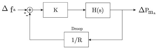
Figure 4. Block diagram of the primary frequency control of Area a.

Alternatively, the equivalent transfer function can be written as

$$G\left(s\right)=\frac{\Delta f_{CO{I}_a}}{\Delta P_{m_a}}=\frac{T_r}{1+s{T}_k}$$

(31)

where $T_r=\frac{-1}{R}$ and $T_k=\frac{-T_r}{K}$.

From Figure 4, the main interest is on $\Delta P_{m_a}$, but it is neither possible to measure it directly nor estimate all the parameters in the diagram.

To solve this problem, a three-step strategy is adopted: first, a rough estimation of $P_{m_a}$ (denoted by $P_{m_a}^r\left(t\right)$) is obtained through data-fitting, second $T_r=\frac{-1}{R}$ and $T_k$ are obtained through model identification (based on $P_{m_a}^r\left(t\right)$), and third the estimation of $P_{m_a}$ is updated through the integration of Equation (31) in the time domain.

In the first step, the data-fitting procedure is applied on $P_{g_a}\left(t\right)$, in an attempt to approximate typical mechanical power responses (obtaining $P_{m_a}^r\left(t\right)$). However, before applying the data-fitting, there are two typical patterns of $P_{m_a}\left(t\right)$ (from the point of view of this methodology) that must be treated differently to determine the procedure to be used. The first pattern is a step change, caused by connection/disconnection of generation. The second pattern includes all the other types of perturbations that do not see a fast change on $P_{m_a}\left(t\right)$. These patterns interfere in the number of reference points needed to apply the data-fitting.

In the case of the first pattern, three reference points are needed to guarantee that the data-fitting is applied only after the step, without smoothing it. The reference points are the last point of $P_{m_a}\left(t\right)$ in steady-state before the perturbation (Point I), the first point of $P_{m_a}\left(t\right)$ in steady-state after the perturbation (Point II) and the first point after the generation step (Point III). The data-fitting is applied between Point III and Point II, in the procedure denominated Strategy 1. In the case of the second pattern, only Point I and Point II are needed, and the data-fitting is applied between them (Strategy 2).

In details, consider the cases simulated with a generic test system and presented in Figure 5. The behavior of the actual $P_{g_a}$ and the actual $P_{m_a}$ of an area that experienced a loss of generation is presented in Figure 5a, while the behavior of an area that suffered a load loss is presented in Figure 5b; both responses are obtained considering the response of a first order generic governor. Please note that the reference points can be fixed also in the $P_{g_a}$ curve.

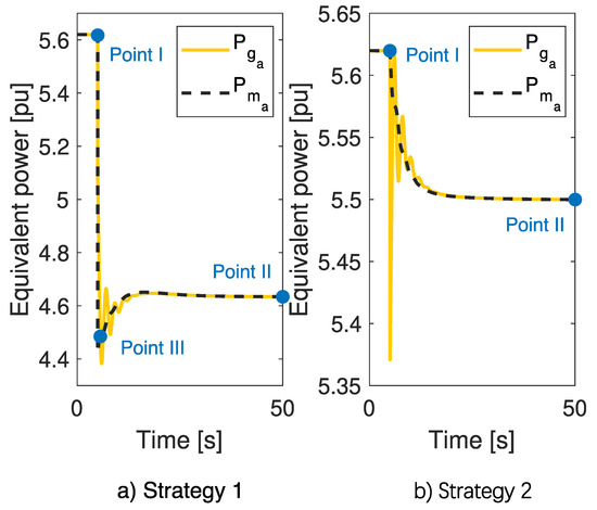
Figure 5. Strategies for the polynomial fitting step.

In this paper, the proposed methodology is tested using computer generated dynamic simulations and, thus, the nature of perturbation and the instant of occurrence of the event are known; such information is used in the selection of the strategy and in the determination of the reference points, according to the procedure previously described. For an automatic real-time procedure, one may make use of event identification methods [6,39,40]. First, a detection of an event triggers the full inertia estimation methodology. Second, the identification of the event as a connection/disconnection of generation triggers the use of Strategy 1, whether the identification of any other event triggers the use of Strategy 2. The automatic determination of the reference points can be done analyzing the second derivative of $P_{g_a}$ (estimated) and adopting a threshold to identify when the signal is in steady state and when it is in transient period. The last sample of the steady-state before and after the perturbation are taken as points I and II, and the first sample of the transient period is taken as Point III (in the case of Strategy 1). Alternatively, one may obtain Point III making use of a technique to estimate the size of a generation loss [41].

After the reference points are selected, the fast frequency transients may be smoothed to allow the electromechanical response to be dominant. To do so, these transients are detected by evaluating the sign of the second derivative of the signal, obtained applying the finite difference method. Then, the fast transients are smoothed with the use of a moving average filter. After a smoother signal is obtained, the responses between points III and II in Strategy 1 and between points I and II in Strategy 2 are approximated with a fifth order polynom

$$P_{m_a}^r\left(t\right)=p_1{P}_{g_a}^5\left(t\right)+p_2{P}_{g_a}^4\left(t\right)+p_3{P}_{g_a}^3\left(t\right)+p_4{P}_{g_a}^2\left(t\right)+p_5{P}_{g_a}\left(t\right)+p_6;$$

(32)

where $p_i,i=1,$ …$,6$ are the coefficients of the polynomial, obtainable using the LSM. In this paper, this procedure is performed with the function fittype in MATLAB.

With the obtained $P_{m_a}^r\left(t\right)$, it is possible to calculate $\Delta P_{m_a}\left(t\right)=P_{m_a}^r-P_{m_a}^{r-st}$, where the subscript $st$ denotes the steady-state before the perturbation. After that, Equation (31) is used to obtain the parameters of $G\left(s\right)$, $T_r$ and $T_k$, through a transfer function identification method. In this paper, this is done through the function tfest in MATLAB, which applies a nonlinear LSM.

After $T_r$ and $T_k$ are obtained, the system of differential equations that describes the primary frequency control in time domain can be integrated to obtain the refined estimation of $P_{m_a}$, denoted here as $P_{m_a}^{est}$. The system can be written as follows:

$$\frac{d{P}_{m_a}^{est}\left(t\right)}{dt}=\frac{1}{T_k}(P_{m_a}^{ref}+\frac{1}{T_r}\Delta f_{CO{I}_a}-P_{m_a}^{est}\left(t\right))$$

(33)

Summarizing, at this point the estimations of the total load power, losses and mechanical power were already obtained. Therefore, it is possible to obtain the equivalent moving power of the Area a:

$$P_{mo{v}_a}^{est}\left(t\right)=P_{m_a}^{est}\left(t\right)-P_{l_a}^{est}\left(t\right)-P_{losse{s}_a}^{est}\left(t\right)$$

(34)

3.3. Estimation of Inertia

With $P_{e_a}\left(t\right)$ measured, ${\delta }_a^{est}\left(t\right)$ and $P_{mo{v}_a}^{est}\left(t\right)$ estimated, Equation (6) can be solved for $H_{CO{I}_a}$ through LSM,

$$H_{CO{I}_a}={\left({\mathbf{A}}^T\mathbf{A}\right)}^{-1}{\mathbf{A}}^T\mathbf{B}$$

(35)

where $\mathbf{A}$ is the vector composed by each sample of $\frac{d^2{\delta }_a^{est}\left(t\right)}{d{t}^2}$ and $\mathbf{B}$ is the vector composed by each sample of $\Delta P_a\left(t\right)=P_{mo{v}_a}^{est}\left(t\right)-P_{e_a\left(t\right)}$.

3.4. Summary of the Methodology

A flowchart summarizing the methodology is presented in Figure 6.

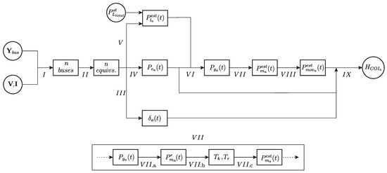
Figure 6. Summary of the methodology.

The steps of the procedure are described below:

I

–Ward Equivalent method to reduce the system around the n buses where PMUs are installed (described in Section 3.1).

II

–Estimation of the n equivalent generators using the “Variance method” (described in Section 3.1).

III

–Calculation of ${\delta }_a^{est}$ through Equation (22).

IV

–Obtainment of the power injected $P_{e_a}\left(t\right)$ from the PMUs at the boundaries.

V

–Estimation of the equivalent load $P_{l_a}^{est}\left(t\right)$ through Equation (25).

VI

–Estimation of $P_{g_a}\left(t\right)$ through Equation (29).

VII

–Estimation of the equivalent moving power

(a)

–Estimation of $P_{m_a}^r\left(t\right)$ through data-fitting (described in Section 3.2.3).

(b)

–Estimation of $T_r$ and $T_k$ through model identification (Section 3.2.3).

(c)

–Estimation of $P_{m_a}^{est}\left(t\right)$ through Equation (33).

VIII

–Estimation of $P_{mo{v}_a}^{est}\left(t\right)$ through Equation (34).

IX

–Estimation of $H_{CO{I}_a}$ through Equation (35).

4. Results

This section is divided in two main subsections. First, tests have been performed to validate the methodology and present details of the procedure; results are presented in Section 4.1. At second, new tests were performed to evaluate the impact of the main steps of the methodology summarized in Figure 6 in the inertia estimation; results are shown in Section 4.2.

4.1. Validation Study

4.1.1. Test System

To validate the methodology, the test system from [26] represented in Figure 7 was simulated in PowerFactory2018, with the two-axis 5th-order IEEE standard detailed Model 2.2 [42] for synchronous machines. Loads were simulated using the constant impedance model, and governors, PSS and AVRs were implemented with generic first order models.

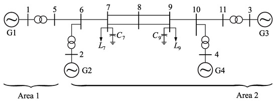
Figure 7. 11-bus test system [26] with areas defined by the proposed methodology.

In the simulations, G1 and G2 oscillate against G3 and G4. However, as it can be seen in Figure 7, the areas will be defined around bus 5 (Area 1) and around bus 6 (Area 2), such that Area 2 is composed by three non-coherent generating units ($G_2,G_3,G_4$). Accordingly, PMUs are assumed as installed at buses 5 and 6, therefore monitoring these two areas. This division aims at testing the methodology proposed with areas containing non-coherent generators. The constants of the primary frequency control simulated are $T_{k_{A1}}=0.0324$, $T_{k_{A2}}=0.0108$ and $T_{r_{A1}}=T_{r_{A2}}=4$, where $A1$ and $A2$ denote Area 1 and Area 2, respectively.

4.1.2. Estimation of the Mean Frequency

A step increase of $10\%$ in the load of bus 9 (see Figure 7) was simulated at $t=5$ s, and two tests were performed. In Test 1, PMUs were considered at the boundary buses 5 and 6, measuring voltages and the injected current at the transmission line 5–6, from both ends. In Test 2, a third PMU was considered installed at bus 9.

In Test 1, the “Variance method” was applied with a selected time window of 2 s around the time the perturbation occurred, considering 0.5 s before and 1.5 s after. The initial guesses for the internal reactances were $x_i=0.1$ p.u. for both areas, and the estimations obtained were $x_{A1}=0.0312$ p.u. and $x_{A2}=0.0644$ p.u, for Area 1 and Area 2, respectively. With the equivalent reactances estimated, the internal voltages $E_{A1}\left(t\right)\angle {\delta }_{A1}\left(t\right)$ and $E_{A2}\left(t\right)\angle {\delta }_{A2}\left(t\right)$ are calculated. The electrical frequencies related to each equivalent generator are determined according to Equation (2), making use of the obtained ${\delta }_i\left(t\right)$ and applying a median filter. In Test 2, Equation (22) is applied to obtain an equivalent behavior for Area 2, taking into account the data acquired at both buses 6 and 9. The weights $W_k$ are assumed equal to one. In other words, the difference between tests 1 and 2 is the consideration in Test 2 of the measurements acquired at bus 9.

To evaluate the dynamic equivalents obtained in both tests, the estimated electrical frequencies of each equivalent machine (denoted by $f_{est}$) are compared with the true mean frequency of each area ($f_{COI}$), computed on the simulation results. Both $f_{est}$ and $f_{COI}$ can be seen in Figure 8 for Area 1 and Figure 9 for Area 2, respectively. In Figure 9, $f_{G2},f_{G3}$ and $f_{G4}$ denote the frequencies simulated of each of the generators of Area 2, $f_{es{t}_{t1}}$ denotes the mean frequency of Area 2 estimated in Test 1 and $f_{es{t}_{t2}}$ denotes the mean frequency of Area 2 estimated in Test 2.

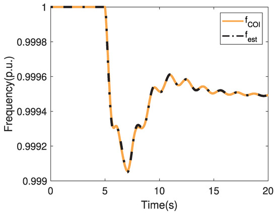
Figure 8. Validation studies—Frequency of Area 1.

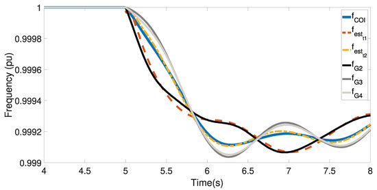
Figure 9. Validation studies—Frequency of Area 2.

It can be observed in Figure 8 that the estimated frequency of Area 1 is very close to the mean frequency of that area; this is expected, since this area has only one generator. Regarding the simulation, the frequency does not come back to nominal values because secondary frequency control is not implemented.

Regarding the estimations of Area 2 in Figure 9, instead, the behavior of $f_{es{t}_{t1}}$ is significantly different from $f_{COI}$. This happens because the measurement point is electrically closer to G2 in relation to the geographical COI of the system, such that the influence of the frequency of G2 ($f_{G2}$) brings the estimated $f_{est}$ closer to its own behavior and far from the COI. Considering a second measurement point (at bus 9) improves the estimation of the mean frequency, as it can be seen with $f_{es{t}_{t2}}$, which is very close to the COI behavior.

This last result show that one may take advantage of PMUs installed inside the area of study. In this case, bus 9 is located closer to the theoretical COI of Area 2; this can be inferred from Figure 7, taking into consideration the radiality of the system and the size of the generators. Therefore, the frequency at bus 9 is a good approximation of the mean frequency of that area, showing that coherent groups does not necessarily have to be individually monitored to provide accurate approximations to the dynamics of the COI.

4.1.3. Estimation of the Moving Power

According to the procedure proposed and summarized in Figure 6, steps IV to VIII are needed to estimate the moving power of each area. In Step IV, the measured voltages and currents at boundary buses 5 and 6 are used to determine $P_{e_{A1}}\left(t\right)$ and $P_{e_{A2}}\left(t\right)$, respectively. In Step V, the voltage behavior of Area 2 is approximated by the voltage behavior of bus 9, where a PMU was already assumed to be installed. In this case, bus 9 is a natural choice not because it is located closer to the COI of the area, but because it is a load bus. How available PMUs might provide measurements that are good approximations to the voltage profile of load buses of the area is system-dependent. The interested reader may refer to [32,43,44].

After the load behavior is estimated, $P_{g_a}\left(t\right)$ is estimated considering $\alpha$ as $5\%$ in Equation (29) (Step VI). Then, $P_{m_a}^r$ is obtained according to Step VII described in Figure 6. During step VIIa, $P_{m_a}^r\left(t\right)$ was obtained with $p_1=-8.25\times {10}^{-7}$, $p_2=3.62\times {10}^{-5}$, $p_3=-5.80\times {10}^{-4}$, $p_4=4.03\times {10}^{-3}$, $p_5=-9.89\times {10}^{-3}$ and $p_6=3.17\times {10}^{-2}$. These parameters provided an index of $0.84$ in the $R^2$ test and $2.9\times {10}^{-3}$ in the RMSE test. During step VIIb, $T_k$ and $T_r$ were obtained with an error smaller than 5% in comparison to the values simulated.

Results are presented in Figure 10, where $P_{m_{sim}}$ stands for the mechanical power coming from the dynamic simulation, $P_m^r$ stands for the estimated mechanical power after the data-fitting step and $P_m^{est}$ stands for the definitive estimation of the mechanical power after the system identification and the integration processes. As it can be seen, the methodology was able to obtain an accurate approximation of $P_m$ for both areas, with a significant improvement moving from $P_m^r$ to $P_m^{est}$.

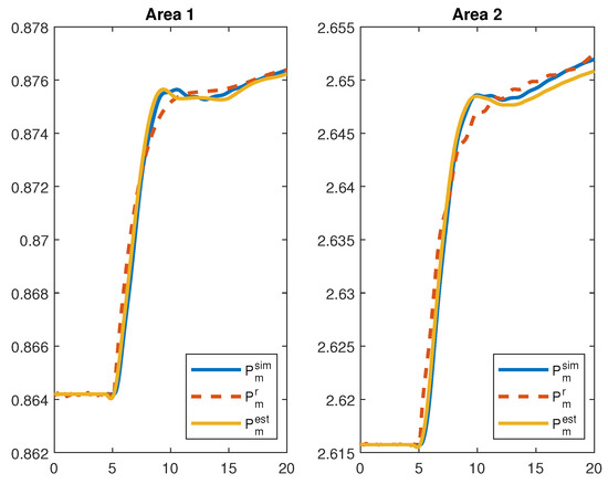
Figure 10. Mechanical Power.

Additionally, results of the estimated $P_l$ and $P_{mov}$ of Area 2 can be seen in Figure 11.

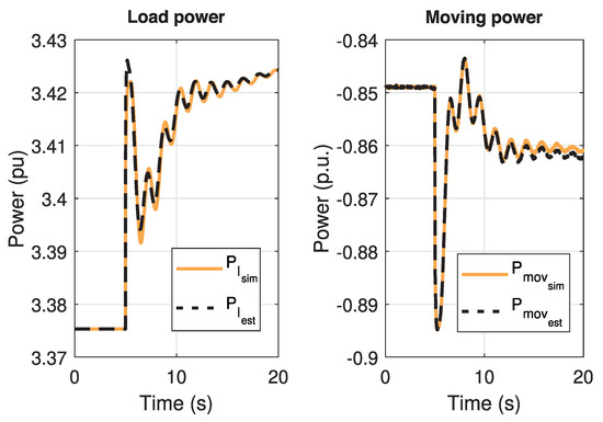
Figure 11. Load power and moving power of Area 2.

4.1.4. Inertia Estimation

A sliding window of 200 samples, with displacement of 20 ms (1 sample per slide) is used to estimate inertia continuously over time. The methodology proposed in this paper is compared with the method proposed in [25] applied at the boundaries of both areas. Results are shown in Figure 12, where ‘A1 expected’ and ‘A2 expected’ denote the input inertia of Area 1 and Area 2 in the simulations, ‘A1 Prop. Method’ and ‘A2 Prop. Method’ denote the estimations obtained with the proposed method and ‘A1 Comp. Method’ and ‘A2 Comp. Method’ denote the results obtained applying the method proposed in [25] directly.

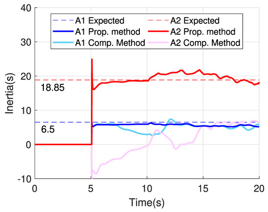
Figure 12. Inertia estimated.

Regarding Area 1, it can be seen that both methods obtain accurate estimations in the first seconds following the perturbation, not surprisingly, as the area is made of a single generator. Regarding Area 2, instead, the proposed method performs well, while the method chosen for comparison obtain wrong results. These results happen because the method proposed in [25] is tailored for estimating machine parameters from measurements obtained at its terminal buses, and it relies on the assumption that the mechanical power has slower behavior in comparison to the electromagnetic power. To apply [25] directly with measurements at boundary buses, it was necessary to assume that the moving power of the area is constant, what does not stand for areas with voltage-dependent loads or perturbations inside, such as Area 2.

Looking at Figure 12, it can also be seen that the estimations obtained with the proposed method lose some accuracy after 5 s. This happens because of two main reasons. First, the moving power estimated also degrades due to the transition of the inertial response to the frequency control (see Figure 10 for Area 2). Moreover, the substantial variations of power and frequency have already faded, and remaining variations are small, impacting on the numerical sensitivity of the method.

4.1.5. Inertia Variation

In this subsection, the simulation has been extended to investigate the behavior of the proposed methodology with the inclusion of RES. At $t=20$ s, a WP generator is connected to bus 10 (Figure 7) injecting the same amount of power of Generator 4 (approximately 720 MW), that is simultaneously disconnected. The WP generator is not contributing to the inertia of the system, such that a decrease on the equivalent inertia of Area 2 happens. Although the events simulated do not generate a power imbalance at the boundaries of the monitored areas, the reactive power imbalance that follows the substitution of $G_4$ by $G_5$ impacts the voltages at the buses of the system and alters the internal flows in Area 2.

The proposed methodology is applied considering PMUs at bus 5, 6 and 9 (as in the previous subsections). In Step VII of Figure 7, the data-fitting method has been applied using the strategy for generation disconnection presented in Section 3.2.3.

The moving power of Area 2 is shown in Figure 13, where $P_{mo{v}_{sim}}$ is the simulated moving power and $P_{mo{v}_{est}}$ is the estimated moving power. As it can be seen, the moving power suffers a perturbation at t = 20 s, but of a much smaller magnitude in comparison to the perturbation at t = 5 s.

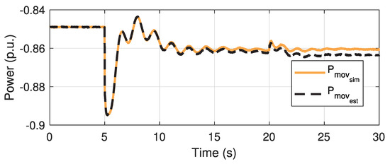
Figure 13. Moving powerestimated (Area 2).

The estimations of inertia can be seen in Figure 14. Please note that the expected value of inertia for Area 2 changes when G4 is disconnected. After the simultaneous events at t = 20 s, the estimations obtained with the proposed method for both areas present a higher standard deviation in comparison to the results obtained following the perturbation at t = 5 s. Less accurate results (following t = 20 s) are natural, since the simultaneous perturbations simulated impose much smaller power imbalance and Rate of Change of Frequency (RoCoF).

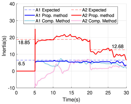
Figure 14. Inertia estimated (inertia variation case).

At t = 20 s, it can be seen that notwithstanding the fact that the measured $P_e$ is slightly affected by the switching of generators, the proposed method was able to react to the event and to identify the change of inertia in Area 2. After 25 s the estimation degrades in consequence of the frequency control, as explained. Please note that the comparison method, assuming slow moving power variation, failed to estimate the inertia of Area 2 through the whole study.

4.2. Performance Evaluation Studies

4.2.1. Test System and Study Cases

To evaluate the performance of the methodology and its critical aspects, new simulations were performed in PowerFactory2018 with the PST 16 Benchmark Test System [27]. The system is composed of 66-bus, 16-synchronous-generator, with total generation installed of 17.9 GW, and total load demand of 15.6 GW. The two-axis 5th-order model for generators (Model 2.2 [42]) was used in the simulations, loads were modelled as constant impedance and the models for controllers can be found in [27].

The test system is represented in a synthetic way in Figure 15, emphasizing the interconnections between the three Areas (A, B, C) and their boundary buses: A1, A2, B1, B2, C1 and C2, where PMUs are assumed to be installed. Main loads are concentrated in area C and power flows from area A and B through the tie-lines. Regarding coherency, the areas divided are large enough to have internal dynamics, depending on the perturbation. Primary frequency control was implemented considering an equivalent $T_k=8$ s and $T_r=0.02$ p.u. for each area.

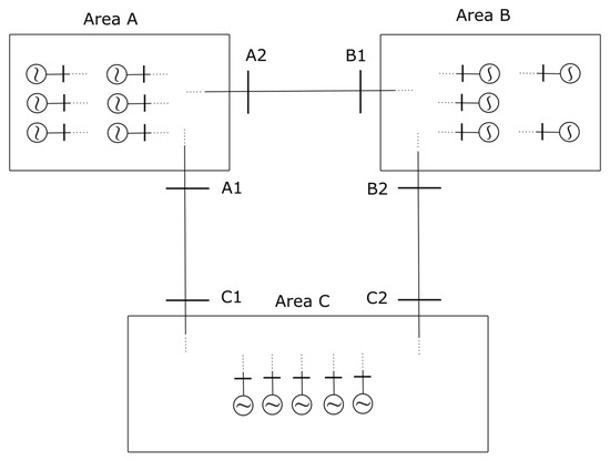
Figure 15. PST 16 Benchmark test system.

Two perturbations have been simulated separately. First, a loss of a generator producing 240 MW and 56 Mvar inside Area B (represents about 3% of the demand of this area and around 1.3% of the total demand). At second, a load shedding of 400 MW and 50 Mvar inside Area B. Random noise signals with normal distribution have been added to the simulated data at the terminals were PMUs were assumed to be installed. The papers [12,45] were taken as reference, and the standard deviations adopted were ${\sigma }_M={10}^{-4}$ for voltage and current magnitudes and ${\sigma }_A={10}^{-6}$ for phase angles. A median filter is applied considering 5 points for phase angles and 10 points for voltage magnitudes.

Each study has been divided in six different cases to assess the sensitivity of the estimation of inertia in relation to the estimations of mean frequency ($f_{COI}$), load behavior ($P_l$) and mechanical power behavior ($P_m$), according to Table 1.

Table 1. Description of the study cases.

	${\mathit{f}}_{\mathit{COI}}$	${\mathit{P}}_{\mathit{l}}$	${\mathit{P}}_{\mathit{m}}$
Case 1	Estimated	Simulated	Simulated
Case 2	Simulated	Estimated	Simulated
Case 3	Simulated	Simulated	Estimated
Case 4	Simulated	Estimated	Estimated
Case 5	Estimated	Estimated	Estimated
Case 6	Estimated	Estimated	Estimated

In Case 1, the mean frequency is estimated while loads and mechanical power behaviors are assumed as monitored. In Case 2, the load behavior is estimated while others are assumed as monitored, and so on in other cases. In Case 5 practical conditions are considered, performing the full methodology with measured data from PMUs at the boundaries and at two internal PMUs in each area (buses A6a, A3a, B3a, B8a, C10a and C2a, referring to [27]). Case 6 assumes full observability.

The selection of the internal buses in Case 5 has been done empirically, aiming at achieving an accurate estimation of the mean frequency with the minimum number of PMUs possible. As one may suppose, the more PMUs the better (Case 6), but the harder to have in practice.

4.2.2. Results

A sliding window of 200 samples (with displacement of 1 sample per slide) is used to estimate inertia continuously over time. To illustrate, the results of Area B in Study 1 are presented in Figure 16. In the legend, $H_{B-C1}$ to $H_{B-C6}$ denote the equivalent inertias of Area B in each of the 6 cases simulated and $H_{B-Expected}$ denote the expected inertia value. As it can be seen, naturally the most practical case ($H_{B-C5}$) deviated most from the expected value. Still, the absolute error was smaller than 10% during most of the time window.

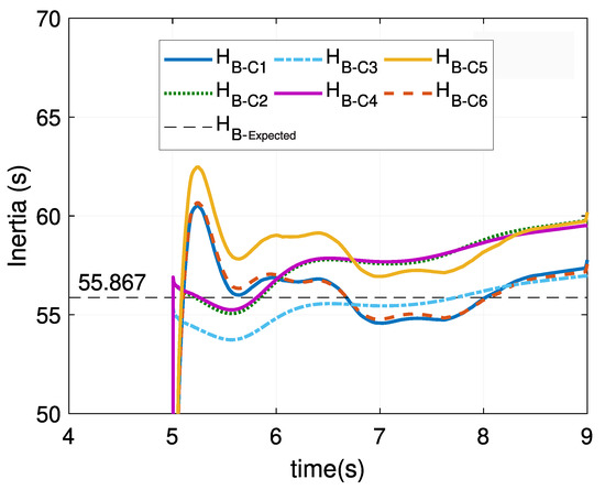
Figure 16. Inertia estimated–Study 1–Area B.

To evaluate the results and discard deviations, a practical criterion is defined: whenever the inertia estimated does not vary more than $1\%$ for 50 consecutive samples (sampling time of 20 ms), a mean average of the estimations is calculated, and the result is considered to be a representative estimation of the constant of inertia of the area. Results can be seen in Table 2, where $e\left(H_i\right)[\%]$ denotes the error on the representative inertia estimated of area $i=A,B,C$ in %, with respect to the constant of inertia at the COI of each area.

Table 2. Representative inertia estimation results.

	Study 1: Loss of Generation			Study 2: Load Shedding
	$\mathit{e}\mathbf{\left(}{\mathit{H}}_{\mathit{A}}\mathbf{\right)}\mathbf{[}\mathbf{\%}\mathbf{]}$	$\mathit{e}\mathbf{\left(}{\mathit{H}}_{\mathit{B}}\mathbf{\right)}\mathbf{[}\mathbf{\%}\mathbf{]}$	$\mathit{e}\mathbf{\left(}{\mathit{H}}_{\mathit{C}}\mathbf{\right)}\mathbf{[}\mathbf{\%}\mathbf{]}$	$\mathit{e}\mathbf{\left(}{\mathit{H}}_{\mathit{A}}\mathbf{\right)}\mathbf{[}\mathbf{\%}\mathbf{]}$	$\mathit{e}\mathbf{\left(}{\mathit{H}}_{\mathit{B}}\mathbf{\right)}\mathbf{[}\mathbf{\%}\mathbf{]}$	$\mathit{e}\mathbf{\left(}{\mathit{H}}_{\mathit{C}}\mathbf{\right)}\mathbf{[}\mathbf{\%}\mathbf{]}$
Case 1	−0.54	−1.07	−3.38	−4.81	−3.20	−8.11
Case 2	4.86	2.05	10.79	2.54	4.88	−8.29
Case 3	4.59	4.64	8.51	7.31	4.16	−2.15
Case 4	9.41	1.85	11.14	8.79	4.86	−7.07
Case 5	12.44	−4.47	9.35	6.06	−1.97	−2.90
Case 6	6.87	1.59	0.95	3.71	−3.30	−1.22

Regarding Case 1, it can be seen that it is possible to achieve accurate estimations of the mean frequency with few PMUs, such that the representative inertia obtained presents errors smaller than $10\%$.

The investigation of the results of Case 2 shows that Area C presented the highest errors. This happens because Area C is the largest area, with larger loads in comparison to the other areas, and therefore estimating the total load behavior based on only 4 PMUs (2 at the boundaries and 2 internal) implies larger approximations. It is worth observing, however, the compensation of this error during the estimation of the moving power in Study 2–Case 4. The same does not happen in Study 1–Case 4.

The results of Case 5 show that the methodology can estimate inertia in practical conditions depending on few PMUs (4 for each area of the test system [27]). The same PMUs have been used to provide data for the mean frequency estimation and to provide data for an approximation of the voltage profile of the area (in the step of load behavior estimation).

The minimum number of PMUs necessary to achieve accurate results depend mainly on the system, the degree of accuracy pretended, and the location where the PMUs will be installed, therefore constituting an optimization problem that may be faced as a topic for future studies. The results of Case 6 show the maximum improvement that can be achieved for this system increasing the number of PMUs.

5. Conclusions

This paper presents a new way of defining areas for dynamic studies, based on synchrophasor measurements. A multi-step methodology is proposed to estimate inertia following perturbations by monitoring an area through its boundaries and possibly a few internal PMUs. First, a measurement-based dynamic equivalent is obtained. At second, an equivalent moving power is estimated, making it possible to study areas that contain perturbations and voltage-dependent loads. At third, equivalent inertia is estimated by the solution of the Swing Equation through LSM.

The determination of the dynamic equivalent brings the first main advantage of the methodology proposed: machines inside the monitored area do not need to be coherent, and in this case the behavior of the COI is estimated. This enables the possibility of delimiting any area by PMUs available on the grid. The methodology also counts with a system-reducing strategy to take into consideration multiple-measurement points. Results show that having spread measurements inside the area provides a better picture of the COI.

Another contribution of the methodology proposed is the estimation of the equivalent moving power of an area. This proposition attends the limitation of methods on the literature that rely on measurements at the terminal of generator groups and on the assumption of slow mechanical power. In the methodology proposed, the estimation of the moving power is done through the estimation of the total load behavior and the estimation of the equivalent mechanical power, which in turn is done through a rough estimation step and an improvement step.

The results obtained with the presented methodology show that accurate estimations of inertia could be obtained considering different types of perturbations with the use of a limited number of PMUs. Future studies include tests with real data, with possible adaptations on Step V of the methodology to estimate the load behavior according to the system.

References

- Arani, M.F.M.; El-Saadany, E.F. Implementing Virtual Inertia in DFIG-Based Wind Power Generation. IEEE Trans. Power Syst. 2013, 28, 1373–1384. [Google Scholar] [CrossRef]
- Bolzoni, A.; Terlizzi, C.; Perini, R. Analytical Design and Modelling of Power Converters Equipped with Synthetic Inertia Control. In Proceedings of the 2018 20th European Conference on Power Electronics and Applications (EPE’18 ECCE Europe), Riga, Latvia, 17–21 September 2018. [Google Scholar]
- Rezkalla, M.; Pertl, M.; Marinelli, M. Electric power system inertia: Requirements, challenges and solutions. Electr. Eng. 2018, 100, 2677–2693. [Google Scholar] [CrossRef] [Green Version]
- AEMO. Inertia Requirements Methodology; Technical Report; Australian Energy Market Operator (AEMO): Melbourne, Australia, 2018. [Google Scholar]
- Malik, O.P. Evolution of Power Systems into Smarter Networks. J. Control Autom. Electr. Syst. 2013, 24, 139–147. [Google Scholar] [CrossRef]
- Kim, D.I.; Chun, T.Y.; Yoon, S.H.; Lee, G.; Shin, Y.J. Wavelet-Based Event Detection Method Using PMU Data. IEEE Trans. Smart Grid 2017, 8, 1154–1162. [Google Scholar] [CrossRef]
- Bosisio, A.; Berizzi, A.; Moraes, G.R.; Nebuloni, R.; Giannuzzi, G.; Zaottini, R.; Maiolini, C. Combined use of PCA and Prony Analysis for Electromechanical Oscillation Identification. In Proceedings of the 2019 International Conference on Clean Electrical Power (ICCEP), Otranto, Italy, 2–4 July 2019; IEEE: Piscataway, NJ, USA, 2019. [Google Scholar] [CrossRef]
- Chow, J.H.; Chakrabortty, A.; Vanfretti, L.; Arcak, M. Estimation of Radial Power System Transfer Path Dynamic Parameters Using Synchronized Phasor Data. IEEE Trans. Power Syst. 2008, 23, 564–571. [Google Scholar] [CrossRef] [Green Version]
- Phadke, A.G.; Bi, T. Phasor measurement units, WAMS, and their applications in protection and control of power systems. J. Mod. Power Syst. Clean Energy 2018, 6, 619–629. [Google Scholar] [CrossRef] [Green Version]
- Chow, J.H. Power System Coherency and Model Reduction; Springer: Berlin/Heidelberg, Germany, 2013. [Google Scholar]
- Fan, L.; Miao, Z.; Wehbe, Y. Application of Dynamic State and Parameter Estimation Techniques on Real-World Data. IEEE Trans. Smart Grid 2013, 4, 1133–1141. [Google Scholar] [CrossRef] [Green Version]
- Wall, P.; Terzija, V. Simultaneous Estimation of the Time of Disturbance and Inertia in Power Systems. IEEE Trans. Power Deliv. 2014, 29, 2018–2031. [Google Scholar] [CrossRef]
- Ashton, P.M.; Taylor, G.A.; Carter, A.M.; Bradley, M.E.; Hung, W. Application of phasor measurement units to estimate power system inertial frequency response. In Proceedings of the 2013 IEEE Power & Energy Society General Meeting, Vancouver, BC, Canada, 21–25 July 2013; pp. 1–5. [Google Scholar] [CrossRef]
- Huang, Z.; Du, P.; Kosterev, D.; Yang, B. Application of extended Kalman filter techniques for dynamic model parameter calibration. In Proceedings of the 2009 IEEE Power & Energy Society General Meeting, Calgary, AB, Canada, 26–30 July 2009; pp. 1–8. [Google Scholar] [CrossRef]
- Cao, X.; Stephen, B.; Abdulhadi, I.F.; Booth, C.D.; Burt, G.M. Switching Markov Gaussian Models for Dynamic Power System Inertia Estimation. IEEE Trans. Power Syst. 2016, 31, 3394–3403. [Google Scholar] [CrossRef] [Green Version]
- Petra, N.; Petra, C.G.; Zhang, Z.; Constantinescu, E.M.; Anitescu, M. A Bayesian Approach for Parameter Estimation With Uncertainty for Dynamic Power Systems. IEEE Trans. Power Syst. 2017, 32, 2735–2743. [Google Scholar] [CrossRef]
- Zhao, J.; Tang, Y.; Terzija, V. Robust Online Estimation of Power System Center of Inertia Frequency. IEEE Trans. Power Syst. 2019, 34, 821–825. [Google Scholar] [CrossRef]
- Zografos, D.; Ghandhari, M.; Eriksson, R. Power system inertia estimation: Utilization of frequency and voltage response after a disturbance. Electr. Power Syst. Res. 2018, 161, 52–60. [Google Scholar] [CrossRef]
- Lugnani, L.; Dotta, D.; Lackner, C.; Chow, J. ARMAX-based method for inertial constant estimation of generation units using synchrophasors. Electr. Power Syst. Res. 2020, 180, 106097. [Google Scholar] [CrossRef]
- Garcia-Valle, R.; Yang, G.Y.; Martin, K.E.; Nielsen, A.H.; Ostergaard, J. DTU PMU laboratory development–Testing and validation. In Proceedings of the 2010 IEEE PES Innovative Smart Grid Technologies Conference Europe (ISGT Europe), Gothenburg, Sweden, 11–13 October 2010; IEEE: Piscataway, NJ, USA, 2010. [Google Scholar] [CrossRef] [Green Version]
- Angioni, A.; Lipari, G.; Pau, M.; Ponci, F.; Monti, A. A Low Cost PMU to Monitor Distribution Grids. In Proceedings of the 2017 IEEE International Workshop on Applied Measurements for Power Systems (AMPS), Liverpool, UK, 20–22 September 2017; IEEE: Piscataway, NJ, USA, 2017. [Google Scholar] [CrossRef] [Green Version]
- Laverty, D.M.; Vanfretti, L.; Khatib, I.A.; Applegreen, V.K.; Best, R.J.; Morrow, D.J. The OpenPMU Project: Challenges and perspectives. In Proceedings of the 2013 IEEE Power & Energy Society General Meeting, Vancouver, BC, Canada, 21–25 July 2013; IEEE: Piscataway, NJ, USA, 2013. [Google Scholar] [CrossRef]
- Smart Grid Investment Grant Program. Factors Affecting PMU Installation Costs; Technical Report; U.S. Department of Energy–Electricity Delivery & Energy Reliability: Washington, DC, USA, 2014.
- Schofield, D.; Gonzalez-Longatt, F.; Bogdanov, D. Design and Implementation of a Low-Cost Phasor Measurement Unit: A Comprehensive Review. In Proceedings of the 2018 Seventh Balkan Conference on Lighting (BalkanLight), Varna, Bulgaria, 20–22 September 2018; IEEE: Piscataway, NJ, USA, 2018. [Google Scholar] [CrossRef] [Green Version]
- Wehbe, Y.; Fan, L.; Miao, Z. Least squares based estimation of synchronous generator states and parameters with phasor measurement units. In Proceedings of the 2012 North American Power Symposium (NAPS), Champaign, IL, USA, 9–11 September 2012; pp. 1–6. [Google Scholar] [CrossRef]
- Kundur, P.; Balu, N.J.; Lauby, M.G. Power System Stability and Control; McGraw-Hill: New York, NY, USA, 1994; Volume 7. [Google Scholar]
- Gonzalez-Longatt, F.; Rueda, J.L. Power Factory Applications for Power System Analysis; Springer Publishing Company: Berlin/Heidelberg, Germany, 2014. [Google Scholar]
- Fan, L.; Wehbe, Y. Extended Kalman filtering based real-time dynamic state and parameter estimation using PMU data. Electr. Power Syst. Res. 2013, 103, 168–177. [Google Scholar] [CrossRef]
- Kalsi, K.; Sun, Y.; Huang, Z.; Du, P.; Diao, R.; Anderson, K.K.; Li, Y.; Lee, B. Calibrating multi-machine power system parameters with the extended Kalman filter. In Proceedings of the IEEE Power and Energy Society General Meeting, Detroit, MI, USA, 24–28 July 2011; pp. 1–8. [Google Scholar] [CrossRef]
- Machowski, J.; Bialek, J.W.; Bumby, J.R. Power System Dynamics, Stability and Control; Wiley: Hoboken, NJ, USA, 2012. [Google Scholar]
- Byrd, R.H.; Schnabel, R.B.; Shultz, G.A. Approximate solution of the trust region problem by minimization over two-dimensional subspaces. Math. Program. 1988, 40, 247–263. [Google Scholar] [CrossRef]
- Regulski, P.; Wall, P.; Rusidovic, Z.; Terzija, V. Estimation of load model parameters from PMU measurements. In Proceedings of the IEEE PES Innovative Smart Grid Technologies, Istanbul, Turkey, 12–15 October 2014; IEEE: Piscataway, NJ, USA, 2014; pp. 1–6. [Google Scholar]
- Alinejad, B.; Akbari, M.; Kazemi, H. PMU-based distribution network load modelling using Harmony Search Algorithm. In Proceedings of the 2012 Proceedings of 17th Conference on Electrical Power Distribution, Tehran, Iran, 2–3 May 2012; IEEE: Piscataway, NJ, USA, 2012; pp. 1–6. [Google Scholar]
- Polykarpou, E.; Asprou, M.; Kyriakides, E. Dynamic load modelling using real time estimated states. In Proceedings of the 2017 IEEE Manchester PowerTech, Manchester, UK, 18–22 June 2017; IEEE: Piscataway, NJ, USA, 2017; pp. 1–6. [Google Scholar]
- Zografos, D.; Ghandhari, M. Power system inertia estimation by approaching load power change after a disturbance. In Proceedings of the 2017 IEEE Power & Energy Society General Meeting, Chicago, IL, USA, 16–20 July 2017; IEEE: Piscataway, NJ, USA; pp. 1–5. [Google Scholar]
- Bliznyuk, D.; Berdin, A.; Romanov, I. PMU data analysis for load characteristics estimation. In Proceedings of the 2016 57th International Scientific Conference on Power and Electrical Engineering of Riga Technical University (RTUCON), Riga, Latvia, 13–14 October 2016; IEEE: Piscataway, NJ, USA, 2016; pp. 1–5. [Google Scholar]
- Vignesh, V.; Chakrabarti, S.; Srivastava, S.C. Power system load modelling under large and small disturbances using phasor measurement units data. IET Gener. Transm. Distrib. 2015, 9, 1316–1323. [Google Scholar]
- Kuivaniemi, M.; Laasonen, M.; Elkington, K.; Danell, A.; Modig, N.; Bruseth, A.; Jansson, E.A.; Orum, E. Estimation of System Inertia in the Nordic Power System Using Measured Frequency Disturbances. In Proceedings of the Lund Symposium on across Borders–Integrating Systems and Markets–CIGRE, Lund, Zweden, 27–28 May 2015; pp. 27–28. [Google Scholar]
- Gao, W.; Ning, J. Wavelet-Based Disturbance Analysis for Power System Wide-Area Monitoring. IEEE Trans. Smart Grid 2011, 2, 121–130. [Google Scholar] [CrossRef]
- Cui, M.; Wang, J.; Tan, J.; Florita, A.R.; Zhang, Y. A Novel Event Detection Method Using PMU Data With High Precision. IEEE Trans. Power Syst. 2019, 34, 454–466. [Google Scholar] [CrossRef]
- Shams, N.; Wall, P.; Terzija, V. Active Power Imbalance Detection, Size and Location Estimation Using Limited PMU Measurements. IEEE Trans. Power Syst. 2019, 34, 1362–1372. [Google Scholar] [CrossRef]
- Proceedings of the IEEE Guide for Synchronous Generator Modeling Practices and Applications in Power System Stability Analyses; IEEE Std 1110-2002 (Revision of IEEE Std 1110-1991); IEEE: Piscataway, NJ, USA, 2003; 72p. [CrossRef]
- Arif, A.; Wang, Z.; Wang, J.; Mather, B.; Bashualdo, H.; Zhao, D. Load Modeling—A Review. IEEE Trans. Smart Grid 2018, 9, 5986–5999. [Google Scholar] [CrossRef]
- Tellez, A.P. Modelling Aggregate Loads in Power Systems. Master’s Thesis, KTH Royal Institute of Technology, Stockholm, Sweden, 2017. [Google Scholar]
- Wall, P.; Gonzalez-Longatt, F.; Terzija, V. Estimation of generator inertia available during a disturbance. In Proceedings of the IEEE Power and Energy Society General Meeting, San Diego, CA, USA, 22–26 July 2012; pp. 1–8. [Google Scholar] [CrossRef]
Publisher’s Note: MDPI stays neutral with regard to jurisdictional claims in published maps and institutional affiliations. |
© 2021 by the authors. Licensee MDPI, Basel, Switzerland. This article is an open access article distributed under the terms and conditions of the Creative Commons Attribution (CC BY) license (https://creativecommons.org/licenses/by/4.0/).