Optimal Battery Energy Storage System Scheduling within Renewable Energy Communities

Abstract

In this work, a strategy for scheduling a battery energy storage system (BESS) in a renewable energy community (REC) is proposed. RECs have been defined at EU level by the 2018/2001 Directive; some Member States transposition into national legislation defined RECs as virtual microgrids since they still use the existing low voltage local feeder and share the same low-medium voltage transformer. This work analyzes a REC which assets include PV generators, BESS and non-controllable loads, operating under the Italian legislative framework. A methodology is defined to optimize REC economic revenues and minimize the operation costs during the year. The proposed BESS control strategy is composed by three different modules: (i) a machine learning-based forecast algorithm that provides a 1-day-ahead projection for microgrid loads and PV generation, using historical dataset and weather forecasts; (ii) a mixed integer linear programming (MILP) algorithm that optimizes the BESS scheduling for minimal REC operating costs, taking into account electricity price, variable feed-in tariffs for PV generators, BESS costs and maximization of the self-consumption; (iii) a decision tree algorithm that works at the intra-hour level, with 1 min timestep and with real load and PV generation measurements adjusting the BESS scheduling in real time. Validation of the proposed strategy is performed on data acquired from a real small-scale REC set up with an Italian energy provider. A 10% average revenue increase could be obtained for the prosumer alone when compared to the non-optimized BESS usage scenario; such revenue increase is obtained by reducing the BESS usage by around 30% when compared to the unmanaged baseline scenario.

1. Introduction

Energy Communities are one of the several legislative and policy tools that could enable the EU citizens to be an active part in the so-called clean energy transition, as fostered by the clean energy package (CEP) [1]. The CEP is a set of eight regulations and directives that aims at shaping the EU energy policies, with an overall target for a 40% greenhouse gas reduction by 2030 and specific targets for a 32.5% of improvement in energy efficiency and for a 32% of the remaining electricity consumption coming from renewable energy sources (RES), both by the same timeframe. The recent “Fit for 55” package of legislative proposals [2], together with the EU green deal package [3], aim to push further these targets by increasing the RED II [4] 2030 target for renewables from 32% to 40% of the EU energy mix, roughly doubling the 2019 level of 19.7%; For what it concerns buildings energy needs, the European Commission is proposing an indicative goal of getting at least 49% of them from RES by 2030; to reach this target there would be the need to steeply increase the use of renewable electricity, heat pumps, solar thermal and district heating.

More specifically, the 2019/944 directive on common rules for the internal electricity market [5] includes new rules to make it easier for citizens to interact with the electricity system as active participants and to improve the uptake of energy communities. Such market participation could be related to the generation, consumption, share or sale of electricity, as well as to the provision of flexibility services through demand-response and storage; all these activities could be done individually or through citizen energy communities. Moreover, the 2018/2001 revised renewable energy directive (RED II) aims to strengthen the role of renewables self-consumers and renewable energy communities, as defined in Art. 22, with a specific attention to household consumers [4].

The establishment of REC would also help increase energy efficiency and RES electricity use in households, harnessing distributed generation energy production at the local level; REC schemes would help citizens to team up and invest in renewable energy assets, fostering the bottom-up development of a more de-fossilized and flexible energy system. At the same time, REC would contribute to fighting energy poverty through reduced energy consumption and lower supply tariffs. REC can take any form of legal entity, among which associations, cooperatives, non- profit organizations and others.

EU Member States (MS) are called to ensure that they can participate in available support schemes, on equal footing with large participants. Italy transposed the general legislative framework for REC as set in Directive 2018/2001, with the Law n.8 28/02/2020, M.D. 16/09/2020 and regulation 318/2020/R/EEL [6,7,8]. The two laws are currently in force as a transient regime, since they will be updated by the transposition law for Directive 2018/2001. Specific rules and limits for the operation of Italian REC, as well as incentive schemes, are described in detail in the following section. The Italian REC could be operated in a very simple way, potentially with no additional efforts; anyway, high level of energy sharing could only be reached by deploying assets that could ensure additional level of flexibility, such as battery energy storage systems (BESS) or controllable loads.

In order to guarantee the expected revenues, an optimal management of the deployed assets should be operated [9,10]; this activity requires forecast for loads and generation, knowledge of the operating cost of the assets and of the market prices for electricity [11].

This paper analyses the techno-economic impacts of the use of mixed integer linear programming (MILP)-based scheduling for a BESS deployed within a small residential REC. In order to define the 24-h ahead BESS scheduling, the MILP receives as inputs loads and generation forecast obtained by using a neural-network based forecasting model, fed with REC historical dataset. To complete the model, a real-time BESS management decision tree-type algorithm was defined, with the objective of putting into operation the MILP-based scheduling and cope with the possible forecast errors. The whole model is recursively applied to a 24-h window, sliding over a 120-days long real dataset. In order to test the model under various conditions, several REC compositions are used. Moreover, different scenarios are defined, and different BESS parameters are tested to find the techno economic optimum for the analyzed REC.

Section 2 of the paper describes the overall legislative and technical framework for REC operation, defines the analyzed REC and thoroughly describes the overall methodology, as well as the various process steps and the involved algorithms. Section 3 reports the main results obtained by this investigation and Section 4 summarizes the main findings and conclusions.

2. Review on the State of the Art

2.1. Machine Learning for Battery Energy Storage Systems

BESS often require algorithmic approaches for both accurate modelling and optimal management of the operation modes. Concerning modelling, although several equivalent circuit models are available in literature [12], practical applications often face the problem of accurate state-of-charge and health level estimation [13,14,15,16] for the accumulator. Indeed, the full system is strongly non-linear and affected by losses, that should be taken into account in all phases of energy conversion; this includes switching devices [17] and magnetic components [18,19]. Concerning management, several figures of merit should be considered, such as reduced degradation of the battery, optimal power flow, and maximum economic revenue. Machine learning plays an important role in this, and several techniques can be used to manage the system behaviour in an optimal way. In [20], authors propose a comparison of different techniques (neural network, support vector machine, logistic regression, and random forest algorithms) for optimal scheduling of the real-time operations of the BESS, which is in general coupled with a higher level grid optimization [21,22,23,24,25]. At the base of the management systems is the knowledge of several electrical, environmental, and economic quantities. Knowledge of these quantities is often limited to historic values, and for this reason, ML based forecasting techniques are often proposed in the literature. In [26] authors propose a proactive prediction of the energy demand of an entire city to be included in an intelligent management system for energy storage and flexible loads. Forecasting through deep learning techniques are also promising with good results for long-short-term-memory (LSTM) networks [27,28,29] and recurrent LSTM [27]. Load forecasting can be performed with convolutional neural networks as well, exploiting the different timescales of the features inherent in the time profile of the phenomenon as an advantage [30,31]. Power quality disturbances could sometime hider the load forecasting capabilities; for this reason, specific classification techniques are often employed [32]. Due to the complexity of the forecasting problem, deep convolutional networks can often benefit from an automated definition of the hyperparameters by means of metaheuristic or evolutionary optimization algorithms [33,34], or networks trained through derivative-free optimization algorithms [35]. Forecasting of energy prices can be important to estimate future trends and optimize the economic aspects of a BESS [36,37,38]. As for any machine-learning approach, the size and quality of the dataset is of fundamental importance to achieving meaningful results and validate the generalization capability towards practical cases of study. Data concerning BESS and renewable energy communities on large scales can be difficult to obtain. For this reason, generative machine learning techniques [39,40,41] can be used to simulate an arbitrarily large REC featuring a variable number of prosumers, also including electric vehicles utilities [42] whose massive deployment is expected in the following years [43].

2.2. Renewable Energy Communities Management Using MILP Techniques

Renewable energy communities (REC) [44,45] are a growing and multifaceted phenomenon which involves one or more activities among production, supply, distribution, sharing and consumption of renewable energy. From a technical point of view, REC can be seen as proper or virtual microgrids, connected to the main grid and composed of controllable and non-controllable loads, renewable energy sources and, possibly, energy storages, among which battery energy storage systems (BESS) [46,47]. In order to optimize REC assets usage a proper power and energy management system is of fundamental importance and thus is the subject of significant ongoing research. Linear programming is often used for both offline and online scheduling and optimization of microgrid assets operation since the underlying economic functions can be expressed in many cases as linear functions of the decision variables [48]. Malysz et al. [49] proposed an optimal control method, based on a mixed-integer-linear-program (MILP) optimization, for the operation of a BESS in a grid-connected electrical microgrid, with the objective of minimizing operating costs and shape demand profile. BESS scheduling optimization using MILP techniques with the objective of increasing RES self-consumption is explored in [50], while the multi-objective optimization carried out by [51] had cost and emissions reductions as main goals. Collaborative approaches are also investigated, involving demand response management of residential loads and optimal scheduling of BESS [52,53] with the objective of establishing P2P energy trading [54,55]. Multi-time-scale models such as in [56] and [57] try to deal with load and generation forecast errors, adjusting in real time the day-ahead scheduling previously prepared.

2.3. BESS CAPEX Evaluation

Considering the cost of BESS is of fundamental importance when evaluating its optimal scheduling. In fact, through the evaluation of CAPEX (capital expenditure) and maximum number of cycles that the BESS could endure, it is possible to obtain a levelized cost of storage (LCOS), that can be defined as the cost of use of the storage for each charged and discharged unit of energy. Several formulations of LCOS exists in literature [58], and several papers have been evaluated [47] in order to gather information on the expected lifetime of BESS [59] and on the calculation of the average costs related to BESS installation [47,60,61].

3. Materials and Methods

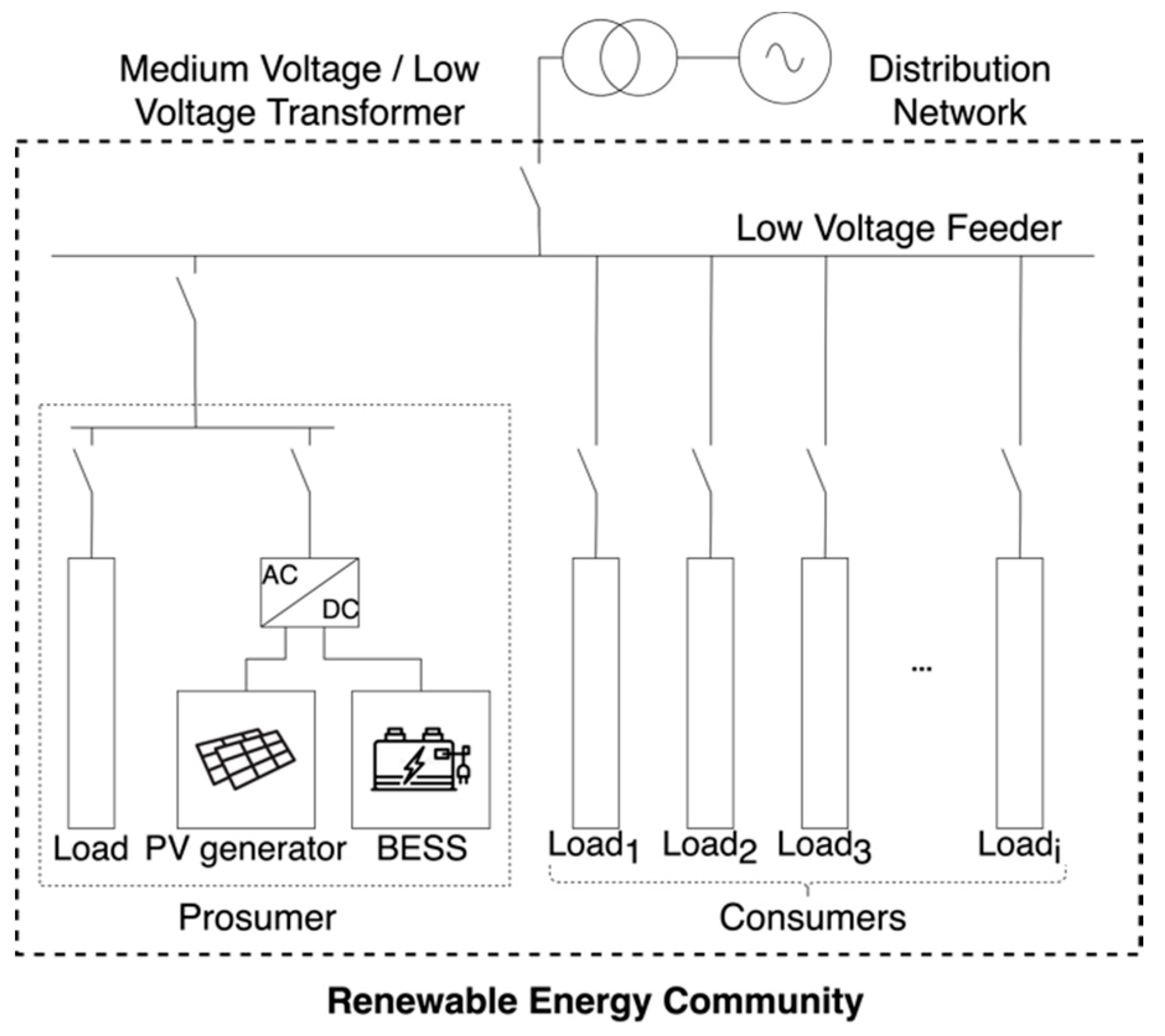
3.1. Italian Renewable Energy Communities: The General Framework and the Analyzed Community

This REC is operated under the framework set by Italian Law n.8 28/02/2020, M.D. 16/09/2020 and regulation 318/2020/R/EEL [6,7,8] that transposed the EU Directive 2018/2001 [4]. Within this framework, a REC is considered as a virtual community, composed by a set of consumers M and a set of RES-powered generators G. The number of consumers is not explicitly limited, while there must be at least one generator for each REC, with a constraint on REC maximum generating power set at 200 kW (to be shared among total set of generators G). It is important to highlight that all the users have to be connected to the public low voltage (LV) distribution grid, that is used to virtually share the energy among them and have to be under the same LV/MV transformer. Each user load is defined by its point of delivery (POD), while a generator could either be defined as stand-alone entity, with its own POD, or could share the POD with a user load, thus under a prosumer framework. In this latter case, the POD energy profile would be seen at time as either a net load or a net generation profile, depending on current load and generation profiles. The BESS, whenever available, has to be deployed behind a POD connected to a generator, as already mentioned above. Figure 1 presents the general architecture of an Italian REC.

The energy shared within this type of REC is defined as the minimum, on an hourly basis (i.e., between 11:00 and 12:00), between the total energy injected in the grid by all REC’s generators and the total energy withdrawn from the grid by all REC’s loads. Because of this virtual approach, generators continue to sell the energy to the grid at day-ahead market prices and users continue to pay the bills for their loads as before. On top of that, a premium of 110 €/MWh is paid to the REC [6,7,8] for the shared energy and has to be divided among the community; no specific rules are defined by the authority on how to share the premium among the REC members, thus this has to be decided by the members itself when the REC is created.

3.2. Case of Study: Simulation of a 5-Households REC Based on Real Measurements

In this work we consider a small REC composed by five households, modeled as non-controllable loads, one rooftop PV system and a BESS; the BESS is considered to be a lithium-ion battery for stationary applications, used with a depth of discharge of 80%. The PV system and the BESS are modeled as a single, integrated system owned by one of the five households, that thus configures as a prosumer, while the other four are simple consumers. The BESS is constrained to be charged only by using energy produced by the PV system, while it can discharge on prosumer loads and on the grid. Discharging on the grid is allowed only when prosumer’s loads are already covered, either by the PV system or by the BESS. Such constraints reflect the existing Italian regulatory framework, in force for the use of BESS in grid-connected applications [60,62].

The data used to characterize the five residential loads and the PV system is derived from a proprietary dataset composed by over 120 days of voltage, current, active and reactive power data, collected from several real loads and PV generators with a 1-min timestep. The revenues related to the sale of energy from PV generation are calculated using prices from the Italian day-ahead electrical market [63], corresponding to the same time period in which the load and generation dataset has been collected. Finally, BESS CAPEX costs have been calculated using data gathered from literature, using the model from [46] to obtain a total cost for BESS using both cell costs, proportional to BESS capacity (in kWh), and inverter costs, related to charging and discharging rated power (in kW). An additional constraint has been set on the inverter size, to match the maximum charge/discharge rates of the BESS. They have been set at $0.5*So{C}_{MAX}$, which is considered as a reasonable estimate for lithium-ion technology in stationary applications. A simplified value of the LCOS was calculated for each combination of BESS capacity and rated power used in the model, with the following equation:

$$LCOS=\frac{CAPE{X}_{BESS}}{2*cycle*So{C}_{MAX}}$$

(1)

The LCOS value is used in the mixed integer linear rdsrrogramming to optimize the BESS scheduling, by adding an estimation of the BESS usage cost to the energy arbitrage operations. Finally, a plausible sharing ratio between prosumer and consumers (as a whole) for the incentives related to PV energy exchanged within the REC was defined and set at 55% and 45%, respectively.

Table 1. Main simulation parameters.

Property	Value of Function	Ref
REC load peak power	13.5 kW	Database
Single household load peak power	2.9 ÷ 4.5 kW
PV gen. peak power	4.6 kW
BESS net capacity	1 ÷ 10 kWh	Own assumption
BESS rated power	0.5 ÷ 5 kW
BESS lifetime cycles	3000	[46]
BESS CAPEX	400 ÷ 3700 €	[46]
BESS LCOS	0.013 ÷ 0.025 €/kWh	Calculated
PV energy value (Day-ahead IT Market)	0.05 ÷ 0.11 €/kWh	[63]
Electricity cost for residential consumers	0.20 €/kWh	[64]
Subsidy on RES electricity shared in REC	0.06 €/kWh (prosumer)	[7], Own assumption
Subsidy on RES electricity shared in REC	0.05 €/kWh (all consumers)

below summarizes all the previously described information.

Table 2. Nomenclature.

$LCOS$	Levelized Cost of Storage (€/kWh)
$CAPE{X}_{BESS}$	Capital Expenditure for BESS (€)
$cycle$	Lifetime charge/discharge cycles
$So{C}_{MAX}$	BESS Max capacity (kWh)
$P_{BESS}^{Ch, MAX}$	BESS max. charge power (kW)
$P_{BESS}^{Dis, MAX}$	BESS max. discharge power (kW)
$P_{PR}^{LOAD}$	Prosumer load (kW)
$P_{PR}^{PV}$	Photovoltaic generation (kW)
$P^{NL}$	Prosumer Net Load (kW)
$P^{NG}$	Prosumer Net Generation (kW)
$P_{REC}^{LOAD}$	Aggregate REC consumers load (kW)
$P_i^{LOAD}$	i-th REC consumers load (kW)
$P_{GRID}^{ }$	Total power virtually exchanged with grid (kW)
$P_{REC}^{NG}$	Net Generation power on REC load (kW)
$P_{BESS}^{CH}$	Total BESS charging power (kW)
$P_{BESS}^{Ch, GR}$	BESS charge from grid (kW)
$P_{BESS}^{Ch, REC}$	BESS charge when REC load is present (kW)
$P_{BESS}^{DIS}$	Total BESS discharging power (kW)
$P_{BESS}^{Dis, GR}$	BESS discharge on grid (kW)
$P_{BESS}^{Dis, REC}$	BESS discharge on REC load (kW)
$P_{BESS}^{Dis, NL}$	BESS discharge on prosumer net load (kW)
$E_{BESS}$	BESS State of Charge (kWh)
${\alpha }_{GR}$$, {\alpha }_{REC}$	Multiplying coefficient for BESS charging
${\beta }_{GR}$$, {\beta }_{REC}$$, {\beta }_{NL}$	Multiplying coefficient for BESS discharging
$P{r}_{INC}^{ }$	Incentive value (€)
$P{r}_{ELEC}^{ }$	Electricity price for residential customer (€/kWh)
$P{r}_{DAM}^{ }$	Electricity price on DAM (€/kWh)
$RE{V}_{REC}^{ }$	Total daily REC revenues (€)
$Incomes$	REC hourly incomes (€)
$Costs$	REC hourly costs (€)
$NPV$	Net Present Value (€)
$DR$	Discount Rate (%)

below summarizes the nomenclature used in this section:

3.3. Optimal BESS Scheduling Process: Methodology Overview

The optimal BESS scheduling process described in this work focuses on maximizing the overall revenues of the REC, considering the hourly values of PV energy on the day-ahead market and the possibility to share energy within the community in order to take advantage of the existing incentives, also leveraging on the use of BESS. The methodology is composed by three successive steps, briefly listed below and then described in full detail in the remaining part of this section:

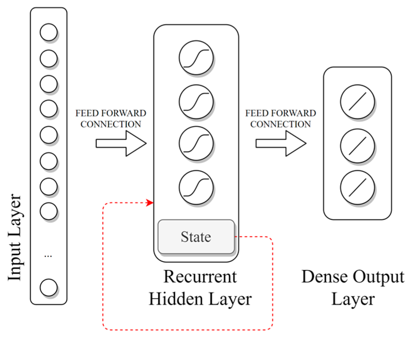
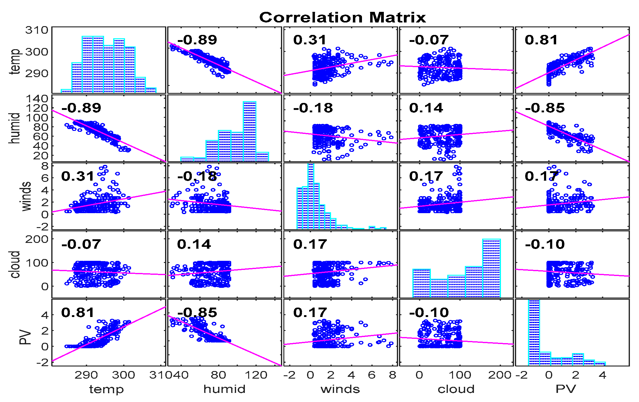
• Definition of 24-h ahead forecast of the hourly trends for PV produced power, prosumer load profile, and aggregated power demand from the rest of the REC. The forecast is obtained with a layer-recurrent neural network, using as inputs the 48 past hourly samples of the quantity to forecast, and the weather forecast for the coming 24 h.
• Optimization of the BESS scheduling within the previously defined REC. The optimization is carried out for the upcoming 24 h with a Mixed Integer Linear Programming (MILP) approach, using as inputs the 24-h ahead forecasts as obtained in Step 1, together with information on PV energy sale price, cost of electricity, LCOS and specific values of BESS characteristics (capacity and rated power). The optimization is obtained by maximizing a revenue function, and the output is the BESS scheduling for the following 24 h in terms of power exchanges with both the PV system, the REC and the grid, with a 1-h timestep.
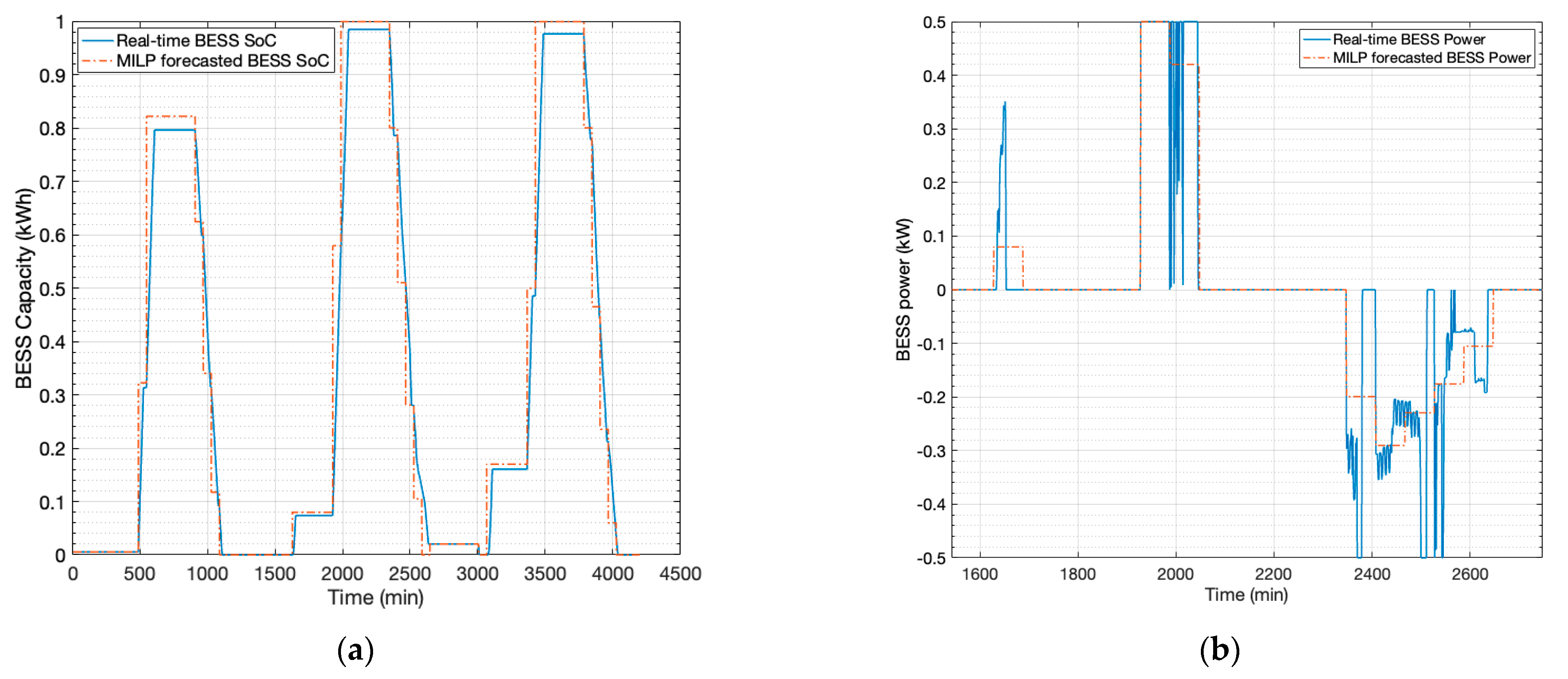
• Real-time BESS management across the 24 h forecasted in Step 1 and 2. The 24-h ahead BESS schedule obtained with the MILP-based, forecast-based optimization is used as a baseline for a real-time BESS management, using real PV production and load curves, with 1-min timestep resolution. A decision-tree algorithm is used to manage BESS charge and discharge phases, with the objective to reach the set points scheduled by the MILP optimization and coping with forecast errors. The final BESS SOC obtained as output from this step is then fed to Step 2 as the initial BESS SOC for the next 24-h ahead optimization process.

3.4. Enriching the Dataset with 24-h Ahead Forecasts: Methodology Overview

Forecasting of the day-ahead quantities relevant for the BESS management is performed through a neural-network based forecasting model. The desired goal is to obtain a reasonably accurate prediction of the hourly trends for PV produced power, prosumer load profile, and aggregated power demand from the rest of the REC. Determination of these quantities can be seen as a classic time-series forecasting problem, for which several considerations must be done to lay out the individual instruments for predicting data.

First, a trend-seasonality-residual (TSR) test must be performed on data, to determine if it exhibit some type of periodic behavior. This analysis is, by itself, a very simple approach to create a forecast (if the assumption that the time series are stationary holds), but can fail for very complex phenomena, resulting in large residuals. However, determining the seasonality period is important to understand the length of the input sequence to be used in any machine-learning based approach.

Second, the exogenous data to be used in the time series must be determined. Very interesting results in the literature correlate energy production to several environmental quantities. Indeed, the most important one is instantaneous normal irradiance on the PV devices. However, considering this quantity would be unfair due to the difficulty of measurement/prediction and the almost unit correlation with power production. Instead, classic weather forecast quantities were used. These quantities exhibit a good correlation with power consumption as well, due to the heavy presence of HVAC loads which responds to environmental changes.

Third and last, the machine-learning architecture must be determined. This step involves the choice of the kind of algorithm/model to use, which, in this work, is a layer-recurrent neural network. This architecture features both a strongly non-linear and dynamic response capability with the inherent advantages related to the training algorithms used in neural networks which can be generalized easily in case of non-uniformly time-spaced data.

Once the forecasting model is determined and trained it is used to create forecasted time-series of the same length (through initial padding) of the original data. The resulting data frame features columns of the real, measured quantities aligned with the 24-h prior forecasts of the same quantities.

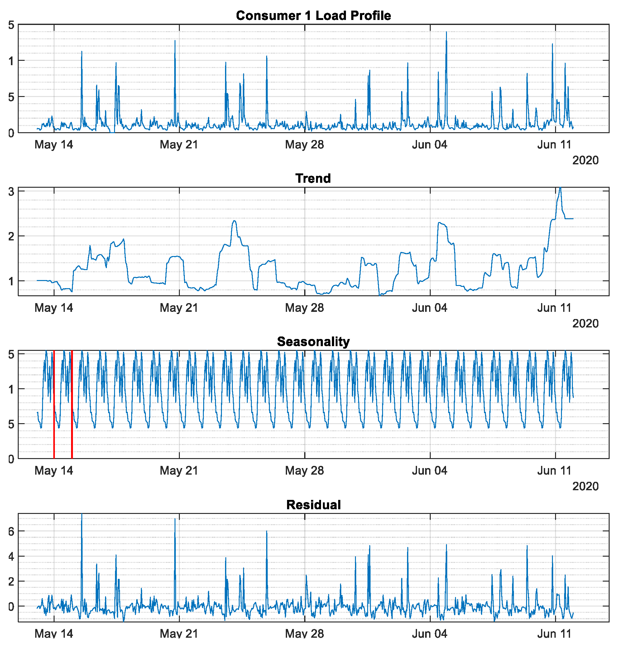
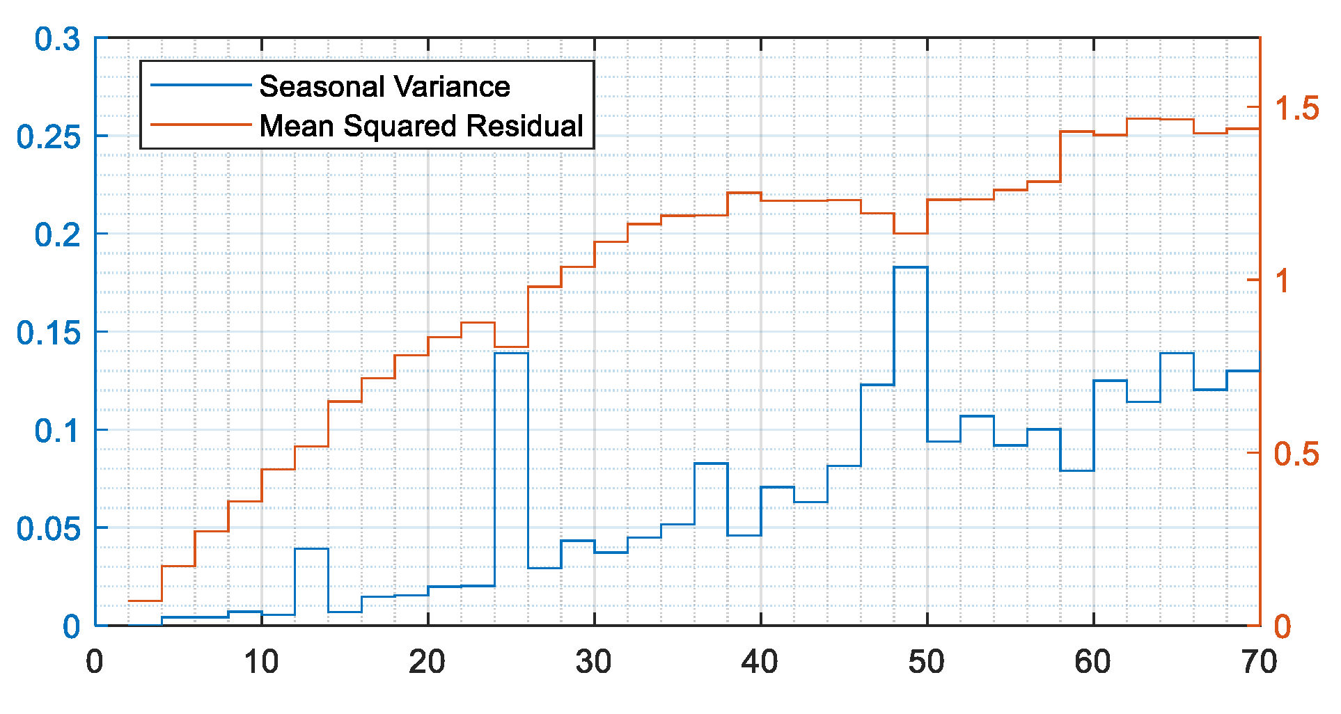
3.5. Trend-Seasonality-Residual Test

A test based on a TSR decomposition is at the base of any autoregressive integrated moving average (ARIMA) model. Time-series forecasting by the means of a neural network can be seen as a non-linear extension (with exogenous inputs) of an ARIMA forecasting. With TSR decomposition, data is split in three time-series with the same length of the original dataset. The only parameter used for the test is the seasonality window. The first component is the trend, which is obtained by using a moving-average filter on the data with window length equal to the seasonality window, and by applying suitable padding on the edges of the vectors to maintain the same length after convolution. The second is the seasonality itself, which is obtained by dividing the de-trended data in time-windows of length equal to the seasonality window and taking the sample-wise average of every window. The resulting average is then repeated to create a vector of the same length of the original data vector. The last is the residual, which is obtained by the difference between the original data and the product between the trend vector and the seasonality vector. An example of the TSR decomposition with a seasonality window size of 24 h is shown in Figure 2. The purpose of applying the TSR decomposition to each component of the dataset is to understand the best sequence-length to be used in the forecasting. Decomposing the series with a too-short seasonality window places the burden of reconstructing the time series on the trend (up to a point where the seasonality is, in general, a constant value). Decomposing the series with a too-long seasonality window raises the residual, leading to seasonality vectors with very little informative content.

A sweet spot for the dataset is found at multiples of 24 and 48 h, as shown in Figure 3. This is expected both due to the natural periodicity of the produced power from the PV devices, and to the anthropic nature of the load profiles.

3.6. Exogenous Data Selection

At the input of the forecasting model, alongside with the past values of the time series to be predicted, a set of exogenous independent data is added to help the forecasting procedure. This data is weather based and is a forecast directly acquired from the OpenWeather Map database. The full dataset includes the 1-day ahead forecast for temperature, pressure, absolute humidity, wind speed, wind direction and cloudiness percentage. In general, all the weather data could be added as exogenous input to the model, relying on the training algorithm to prune the non-useful data. A different approach consists in observing the correlation between the time series and the data to be forecasted. An example is shown in Figure 4 for the forecasting of the produced PV power. As can be seen, the produced PV power has a good linear correlation with both temperature and humidity, and unexpectedly, a very low correlation with the cloudiness index. This is probably due to the more local nature of the interaction between cloud shading and PV devices, making the effective correlation between a regional cloudiness forecast with the produced PV power low. Using as exogenous inputs weather data with low significance has the effect of inducing a noise source in the system that needs to be filtered by the training algorithm itself, leading to slower convergence and possibly local minima entrapment. For this reason, only the values of temperature and humidity are considered as exogenous inputs.

3.7. Neural Architecture Determination

Considerations up to this point determined the optimal window length for past occurrences of the time series to be forecasted and the correlation of the future values with the exogenous weather data. This information can be used to create a very wide range of models for forecasting, including both static, dynamic, linear and non-linear. For the purpose of this work, a dynamic neural model is used. The neural architecture chosen is a layer-recurrent neural network. This architecture, shown in Figure 5, is derived from a feed-forward neural network by adding a delay-tapped feedback loop from the output of each hidden neuron to the input of the layer itself. This allows the network to exhibit a non-linear dynamic behavior, making it a prime candidate to represent systems with non-linear state-space equations. The full input of the neural network is composed by the 48 past hourly samples of the quantity to forecast, and the weather forecast for the next 24 h of temperature and humidity, for a total of 48 + 24 + 24 = 96 inputs. The outputs of the network are the 24 h prediction (thus a sequence-to-sequence forecasting paradigm) of the desired variable.

3.8. REC Power Balance

All the REC members are connected and exchange electrical energy with the main grid, thus the power balance is always obtained considering grid contribution, as described by (2).

$$(P_{PR}^{LOAD}\left(h\right)-P_{PR}^{PV}\left(h\right))+\left(\alpha \left(h\right)*P_{BESS}^{CH}\left(h\right)-\beta \left(h\right)*P_{BESS}^{DIS}\left(h\right)\right)+P_{REC}^{LOAD}\left(h\right)=P_{GRID}^{ }\left(h\right)$$

(2)

The variable $P_{REC}^{LOAD}$ represents the total load request from all the community members:

$$P_{REC}^{LOAD}\left(h\right)={\displaystyle \sum }_{i=1}^M{P}_i^{LOAD}\left(h\right)$$

(3)

To model the fact that the BESS cannot be simultaneously charged and discharged, the variables $\alpha \left(t\right)$ and $\beta \left(t\right)$ describe for each time h the behavior. The variables are binary (1 or 0) and cannot be both 1 at the same time.

The prosumer is seen by the main grid as either a net load or a net generator, depending on the time, as described in (4). The BESS is enabled to charge only when the prosumer is a net generator; no constraints on the discharge are set, thus it can discharge both on the prosumer load and on the grid.

$$\{\begin{array}{c}{P}^{NL}\left(h\right)=P_{PR}^{LOAD}\left(h\right)-P_{PR}^{PV}\left(h\right) if P_{PR}^{LOAD}\left(h\right)>P_{PR}^{PV}\left(h\right)\\ P^{NG}\left(h\right)=P_{PR}^{PV}\left(h\right)-P_{PR}^{LOAD}\left(h\right) if P_{PR}^{PV}\left(h\right)>P_{PR}^{LOAD}\left(h\right)\end{array}$$

(4)

3.9. Mixed Integer Linear Programming-Based Economical Optimization of BESS Scheduling

MILP is used to solve constrained optimization problems which contains an objective function, a set of variables, of which some are not discrete and a set of constraints, that can be equations and inequalities. The scope of the optimization is to find the best solution for the objective function within the set of solutions that satisfy all the constraints. The mathematical formulation of a MILP problem is expressed as follows:

$$\begin{gathered} \mathrm{Objective}: maximize=Cx \\ \mathrm{Constraints}: A*x\le b \\ {x}_{min}\le x\le x_{max} \end{gathered}$$

(5)

where $x \in {\mathbb{Z}}^n$ C, b are vectors and A is a matrix.

The objective function is formulated to maximize the REC revenues $RE{V}_{REC}^{ }$ within the considered 24-h ahead timeframe. These revenues are obtained as the difference between incomes and costs. Costs are related to the use of BESS and are defined by LCOS; incomes are related to the sale of PV net surplus to the grid, to the incentive related to the energy exchanges within the REC and finally to the avoided purchase of electricity from the grid by the prosumer. The daily revenue is formulated as follows:

$$RE{V}_{REC}^{ }\left(day\right)={\displaystyle \sum }_{h=1}^{24}Incomes\left(h\right)-Costs\left(h\right)$$

(6)

$$\begin{gathered} Incomes\left(h\right)=(P_{GR}^{NG}\left(h\right)+P_{BESS}^{Dis, GR}\left(h\right))*P{r}_{DAM}^{ }\left(h\right)+(P_{REC}^{NG}\left(h\right)+P_{BESS}^{Dis, REC}\left(h\right)) \\ *\left(P{r}_{DAM}^{ }\left(h\right)+P{r}_{INC}^{ }\left(h\right)\right)+P_{BESS}^{Dis, NL}\left(h\right)*P{r}_{ELEC}^{ }\left(h\right) \end{gathered}$$

(7)

$$\begin{gathered} Costs\left(h\right)=LCOS*\left(P_{BESS}^{Ch, GR}\left(h\right)+P_{BESS}^{Ch, REC}\left(h\right)+P_{BESS}^{Dis, NL}\left(h\right)+P_{BESS}^{Dis, GR}\left(h\right) \\ +P_{BESS}^{Dis, REC}\left(h\right)\right) \end{gathered}$$

(8)

The constraints related to BESS operation are formulated as follows:

$$0\le P_{BESS}^{Ch, GR}\left(h\right)\le {\alpha }_{GR}\left(h\right)*\min \left(\max \left((P^{NG}\left(h\right)-P_{REC}^{LOAD}\left(h\right)\right),0\right),P_{BESS}^{Ch, MAX})$$

(9)

$$0\le P_{BESS}^{Ch, REC}\left(h\right)\le {\alpha }_{REC}\left(h\right)*\min \left(P^{NG}\left(h\right),P_{REC}^{LOAD}\left(h\right),P_{BESS}^{Ch, MAX}\right)$$

(10)

$$0\le P_{BESS}^{Dis, GR}\left(h\right)\le {\beta }_{GR}\left(h\right)*P_{BESS}^{Dis, MAX}$$

(11)

$$0\le P_{BESS}^{Dis,REC}\left(h\right)\le {\beta }_{REC}\left(h\right)*\min \left(\max \left((P_{REC}^{LOAD}\left(h\right)-P^{NG}\left(h\right)\right),0\right),P_{BESS}^{Dis, MAX})$$

(12)

$$0\le P_{BESS}^{Dis,NL}\left(h\right)\le {\beta }_{NL}\left(h\right)*\min \left(P^{NL}\left(h\right),P_{BESS}^{Dis, MAX}\right)$$

(13)

where, respectively, (10) and (9) define the power limits to charge the BESS when either load from REC is present or not. From the optimization point of view, it is important to distinguish between these two situations, because the part of PV surplus energy $P^{NG}\left(t\right)$ that is used to charge the BESS cannot be exchanged with the REC or sold to the grid; thus, it is important to allow the MILP to correctly choose the optimal timing by differentiating the various possible situations in order to correctly address the corresponding revenue streams. Equations (12) and (13) instead define the power limits to discharge the BESS on the grid when either load from REC is available or not. In this case, the differentiation is needed to correctly address the revenue streams as well. All these equations are to be used in Equations (7)–(9) to define if the energy is shared among the REC or not, and thus if it is entitled for the payment of the incentive or not, in top of the day-ahead market price. Finally, Equation (14) defines the power limits for BESS discharge on prosumer’s net load. All the non-zero constraints in (9)–(13) have a multiplying coefficient in the form of ${\alpha }_k\left(t\right)$ or ${\beta }_k\left(t\right)$. As previously stated, the value of these coefficients can be either 0 or 1 but not both 1 at the same time, and are used to avoid simultaneous charging and discharging of the BESS during the optimization process.

The other constraints set on BESS behavior concern its state of charge (SoC): the maximum and minimum SoC limits are defined in the following (14), while the variation of BESS SoC as a function of power exchanges is defined in (15).

$$0\le E_{BESS}\left(h\right)\le So{C}_{MAX}\left(h\right)$$

(14)

$$\begin{gathered} E_{BESS}\left(h\right)=E_{BESS}\left(h-1\right)+(P_{BESS}^{Ch, GR}\left(h\right)+P_{BESS}^{Ch, REC}\left(h\right)-P_{BESS}^{Dis, NL}\left(h\right)-P_{BESS}^{Dis, GR}\left(h\right) \\ -P_{BESS}^{Dis, REC}\left(h\right)) \end{gathered}$$

(15)

The last two constraints set for MILP optimization are described by (16) and (17), regarding the PV net surplus from prosumer. They are represented by $P_{REC}^{NG}\left(t\right)$ and $P_{GR}^{NG}\left(t\right)$, that respectively describe the power virtually exchanged with the REC and the power simply sold to the grid.

$$P_{REC}^{NG}\left(h\right)=\max \left((P_{GR}^{NG}\left(h\right)-P_{REC}^{LOAD}\left(h\right)\right),0)-P_{BESS}^{Ch, GR}\left(h\right)-P_{BESS}^{Ch, REC}\left(h\right)$$

(16)

$$P_{GR}^{NG}\left(h\right)=P^{NG}\left(h\right)-P_{REC}^{NG}\left(h\right)$$

(17)

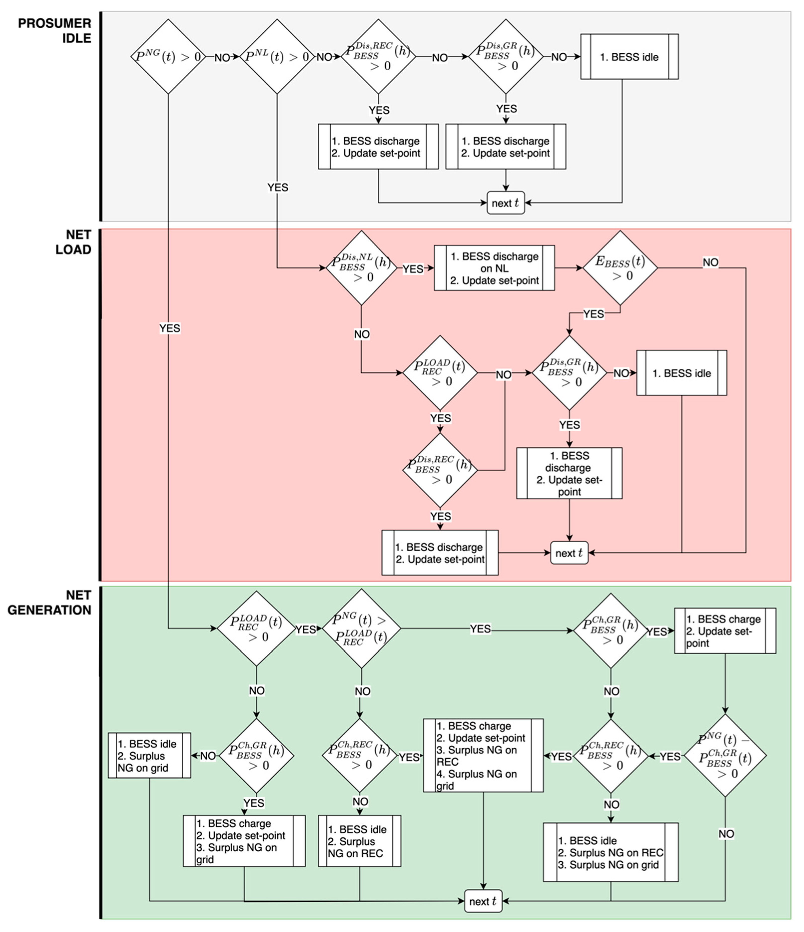
3.10. Real-Time BESS Management: Methodology

The real-time BESS management algorithm is defined to reach the set-points defined by the MILP optimization for each of the following 24 h, while managing the forecast errors related to PV power generation and prosumer and REC aggregated load curves. The set-points refer to the average power exchanges, during the hour h, between the BESS and the NL (discharge, $P_{BESS}^{, Dis, NL}\left(h\right)$), the BESS and the REC (discharge, $P_{BESS}^{Dis, REC}\left(h\right)$ and charge, $P_{BESS}^{ Ch, REC}\left(h\right)$) and the BESS and the Grid (discharge, $P_{BESS}^{Dis, GR}\left(h\right)$ and charge, $P_{BESS}^{, Ch, GR}\left(h\right)$). By following the charging and discharging set-points as suggested by the MILP, we ensure that the BESS scheduling takes into account parameters such as price of energy and forecast on the expected availability and need for energy. This task is performed by a decision tree algorithm, operated with a 1-m timestep t, the same of the dataset used. This higher data resolution allows to get a view on the effect on BESS management system of much less smoothed load and power curves, when compared to 1-h averages of the same data. Using this approach, short and intense power peaks are present and the transition zones between prosumer net generation and net load are much less defined. After each step t all the differences between real power exchanges and the expected ones, as defined by the set-points, are updated. The power exchanges continue until such differences are completely compensated, or the 1-h block h ends. In the latter case, the set-points are updated to the new values related to hour (h+1) and the process starts again. As a consequence of using forecasted data for the MILP-based optimization and real data for the here described real-time BESS management, it is possible that the algorithm couldn’t manage to reach the expected set point. The flowchart in Figure 6 below describes the main algorithm steps, while the sub-algorithms triggered by the various set points are described in the followings.

BESS power exchanges are always limited by a set of parameters: some inherently technical such as the state of charge $E_{BESS}\left(t\right)$ and the rated power $P_{BESS}^{Dis, MAX}$ and $P_{BESS}^{Ch, MAX}$, others related to the availability of surplus energy from PV system $P^{NG}\left(t\right)$ or to the availability of loads on which to discharge such as $P^{NL}\left(t\right)$ and $P_{REC}^{LOAD}\left(t\right)$ and finally of course by the set points previously described. Once that the power exchange involving the BESS in the step t is defined, the SoC is updated. If the prosumer acts as a net generator, thus $P^{NG}\left(t\right)>0$, the algorithm evaluates if there is still available power beside the part used to charge the BESS; if so, it is accounted as energy shared within the REC up to the limit defined by the underlying $P_{REC}^{LOAD}\left(t\right)$, and the exceeding part $P_{GRID}^{NG}\left(t\right)$ is considered as sold to the grid. The following equations explain in details the above-described procedure for the case in which $P^{NG}\left(t\right)>0$, the set-point $P_{BESS}^{ Ch, REC}\left(h\right)>0$, and $P_{REC}^{LOAD}\left(t\right)>0$: in this case the BESS is managed to charge, as described by (18), and the SoC is updated accordingly to (21). The power exchanges within the REC and with the grid are respectively described by (19) and (20).

$$\begin{gathered} P_{BESS}^{Ch, REC}\left(t\right)=\min \left((So{C}_{MAX}-E_{BESS}\left(t-1\right)\right)*60, (P^{NG}\left(t\right)- \\ {P}_{REC}^{LOAD}\left(t\right)), P_{BESS}^{Ch, MAX}, P_{CER}^{TGT, Ch}\left(h\right)) \end{gathered}$$

(18)

$$P_{REC}^{NG}\left(t\right)=\min \left(\left(P^{NG}\left(t\right)-P_{BESS}^{Ch, REC}\left(t\right)\right),P_{REC}^{LOAD}\left(t\right)\right)$$

(19)

$$P_{GRID}^{NG}\left(t\right)=\min \left(\left(P^{NG}\left(t\right)-P_{BESS}^{Ch, REC}\left(t\right)-P_{REC}^{NG}\left(t\right)\right),0\right)$$

(20)

$$E_{BESS}\left(t\right)=E_{BESS}\left(t-1\right)+\frac{P_{BESS}^{Ch, REC}\left(t\right)}{60}$$

(21)

The other cases, described in Figure 6, are managed similarly, and not described here for sake of brevity.

3.11. Description of the Macro-Scenarios and the Operative Scenarios

A set of three different scenarios have been evaluated in this work to better understand the impact of BESS use on REC revenues:

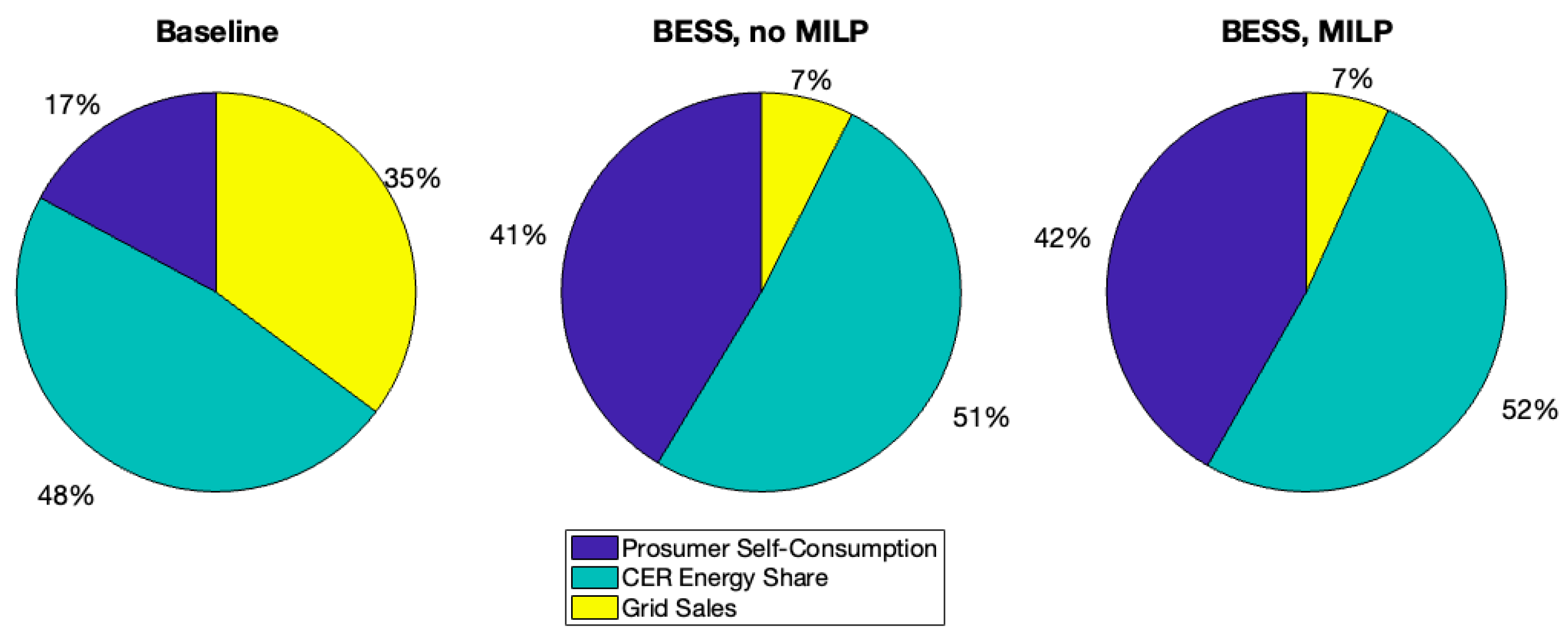
• Baseline: in this scenario, the REC is composed by only PV generator and loads, and no management is applied. This represents the minimal set-up for REC operation.

• BESS, no MILP: in this scenario, the BESS is deployed in the REC, owned by the prosumer and installed within the PV system. No generation and loads forecast, nor BESS management is applied (except for keeping within power and SoC limits), just the basic opportunity charging with the BESS charging whenever $P^{NG}>0$, and discharging whenever $P^{NL}>0$ or $P_{REC}^{LOAD}>0$, or both.

• BESS, MILP: all the previously explained three-steps methodology is applied in this scenario, the load and generation forecasts, the MILP optimization and the real-time BESS management.

In order to take into account the possible REC configuration that could be found in a real life set-up, five different REC have been evaluated, by the permutation of the prosumer within the set of residential loads available; all these permutations were applied to the 120-day loads and generation database as well as to the related forecasts. Ten values of BESS capacity and ten rated BESS power were evaluated in all the BESS-based scenarios, to get perspective on their impact on REC operations and revenues, as described in Table 1. Revenues were calculated using the following NPV formula, using a discount rate (DR) of 5% and a 20-year lifetime:

$$NPV=-CAPEX+{\displaystyle \sum }_{i=1}^{20}\frac{\left(revenue{s}_i^{MILP, BESS}-revenue{s}_i^{BASELINE}\right)-cost{s}_i}{{\left(1+DR\right)}^i}$$

(22)

It can be noticed that the NPV calculation refers only to the part of the revenues enabled by the deployment of the BESS; such revenues are conventionally attributed to the prosumer since in this work it is considered as the BESS owner.

Whenever the cumulative use of BESS reached the maximum lifecycle capacity as defined by (23), it has been considered the deployment of a new one, and the costs related to BESS CAPEX were accounted to the specific year in the overall cash flow.

$$BES{S}_{capacity}^{MAX}=2*cycle*So{C}_{MAX}$$

(23)

4. Results

4.1. Dataset Enrichment: Optimal Neural Network Hyperparameters Sizing

The experimental dataset features three variables to be determined: the produced PV power, the self-consumed power from the prosumer, and the aggregated consumed power from the REC.

Although both seasonality and exogenous data considerations applies to either of these cases, the optimal sizing of the neural network hyperparameters is slightly different. For this reason, three different neural networks were created, sized and trained for the different purpose of predicting produced PV power, individual self-consumed power and aggregated consumed power. Through a heuristic approach, already used with success in different other works, the optimal sizing for hidden layer number of neurons and number of delay-taps is shown in

Table 3. Optimal hyperparameters for the three Layer-Recurrent Neural Networks.

	Hidden Layer Size	Delay-Taps
PV Production	3	1
Consumed Power	9	2
REC Consumed Power	5	1

.

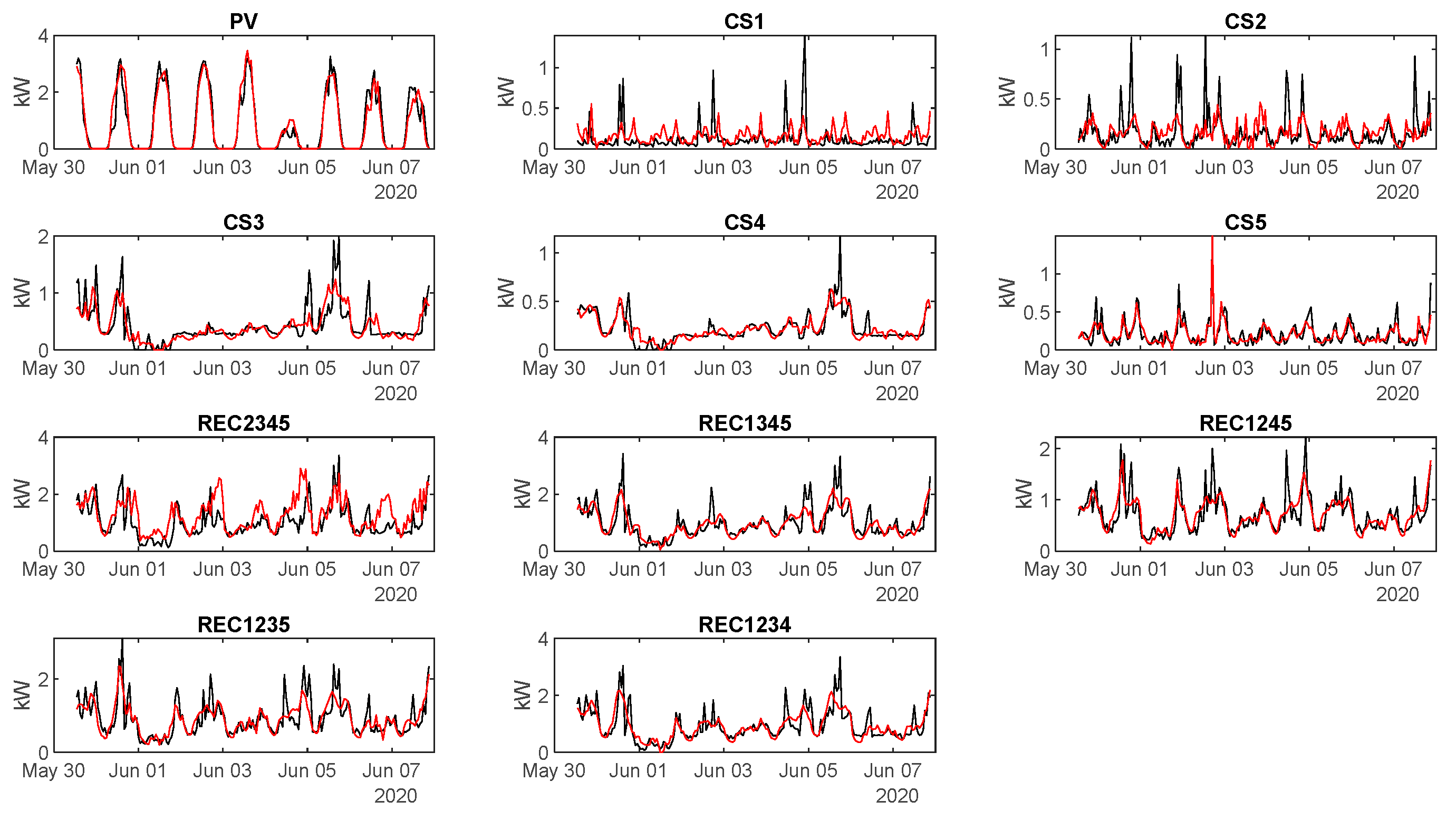
4.2. Dataset Enrichment: Forecasting Accuracy

Since no prior constraint is given on the role of consumer or prosumer, the problem of forecasting can be formulated considering either of the five households as prosumer and the remaining four as the components of the REC. Thus, the number of time-series to be forecasted is a total of 11:

• 1 PV power production
• 5 Consumed Power from the individual households
• 5 REC Consumed Power from the remaining households

The performance of forecasting varies, especially considering that some households show profiles with a much less regular behavior if compared to the others. In scenarios where these irregular households are the prosumers, forecasting is difficult. However, when the irregular households belong to the REC, forecasting the cumulative power is easier and achieves better performance. An extract of about 8 days showing the comparison between real quantities (black) and forecast quantities (red) is shown in Figure 7.

The mean error related to the forecasted quantities has been calculated using the Mean Absolute Percentage Error (MAPE) formulation:

$$MAPE=\frac{{\sum }_{t=1}^n\left|\frac{P_{FORE}\left(t\right)-P_{REAL}\left(t\right)}{P_{REAL}\left(t\right)}\right|}{n}$$

(24)

On average, across the 120 days of dataset and for the various consumers and REC compositions, the obtained values are:

• Single household load MAPE: 19.9–34.3%
• REC composed by the remaining households MAPE: 26.1–29.7%
• PV power production MAPE: 8.2%

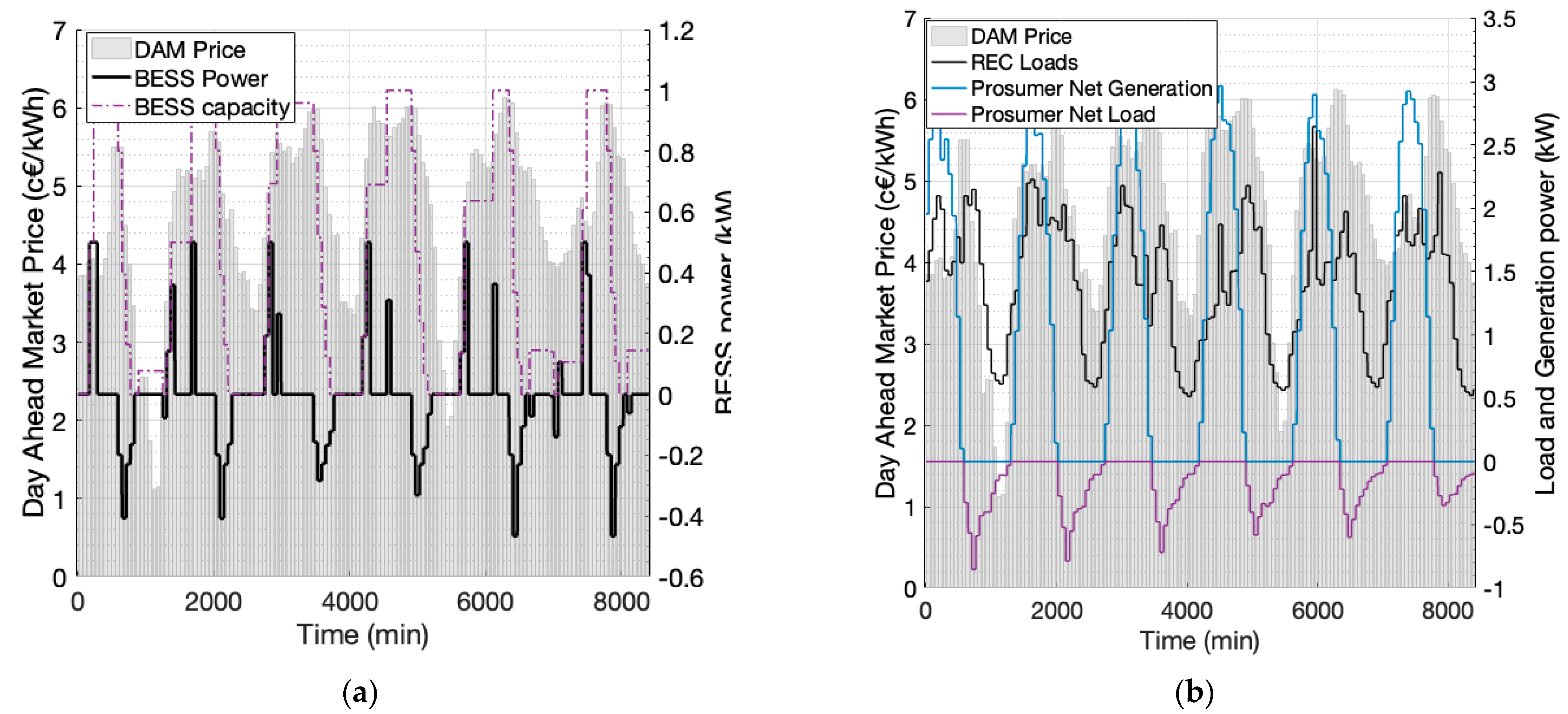
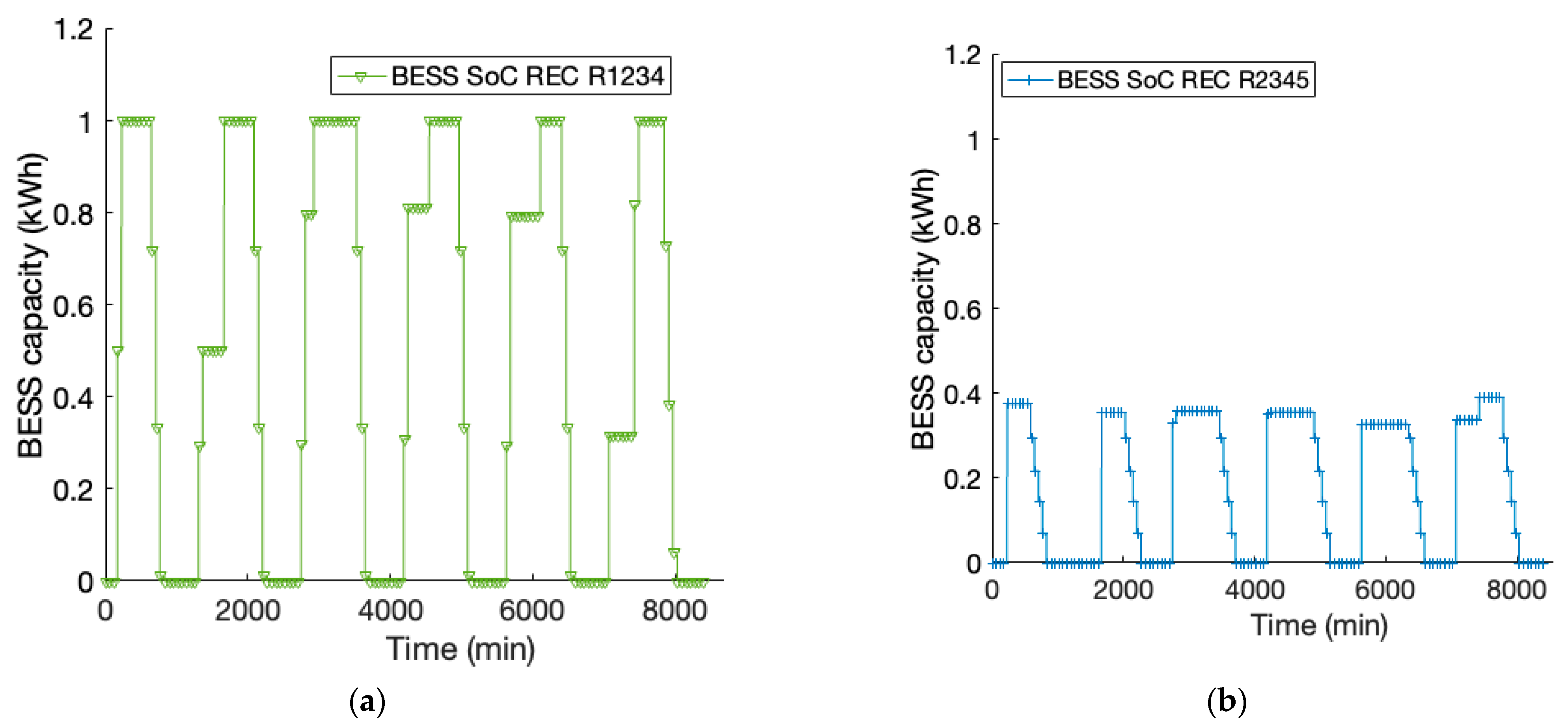
4.3. MILP Optimal Scheduling

Simulations are performed under a variety of conditions, using the forecasted data for loads and PV generation to test the optimal BESS scheduling capability. BESS is charged using PV surplus energy, that otherwise would have been discharged on the grid, possibly accounted as shared energy within REC if loads from other REC members are actives at the same time. In order to maximize REC revenue, BESS has to be charged when energy price is low on DAM and possibly when no loads from other REC members are active, in order not to lose the relative incentive; BESS has to be discharged in an opposite situation, when electricity price is high on DAM and other REC members’ loads are present, in order to get the additional incentive. Moreover, BESS can be discharged on prosumer net load; in this case the revenue is the avoided cost for electricity purchase. In the specific situation investigated in this work, the revenue related to the avoided electricity purchase is the highest one, followed by the one related to the energy shared within the REC. The least remunerative solution sees the PV surplus energy sold to the grid without being accounted as shared energy within the REC. Figure 8 below shows 6 days of MILP output: on the left BESS total power exchanges are reported in black and the corresponding BESS SoC in purple, while the DAM price values are reported as gray bars. It is to be noticed that the algorithm most of the times schedules the BESS to charge in low-price periods and also schedules it to discharge either on prosumer net load or in high-price periods, as should be expected. On the right, instead, the REC loads curve is shown together with the prosumer’s net load and net generation curves, across the same 6 days. These are the main inputs, together with the various electricity prices, incentives and LCOS, that are used by the MILP to optimize the BESS scheduling with the objective of REC revenues maximization.

Figure 8 refers to one of the five analyzed REC compositions; each composition has different inputs for the MILP and this in turns affects optimization results; Figure 9 shows the BESS SoC curve for two out of the five different REC compositions analyzed in this study, over the same 6 days.

4.4. Real-Time BESS Management Operation

The optimal scheduling calculated using MILP methodology with forecasted data has then been tested against real data with 1-min timestep. The decision tree algorithm used in this phase has the objective of reaching the set-points previously calculated by the MILP for the following 24 h, while coping with possible forecast errors. Figure 10a below shows the real-time SoC curve, compared with the one proposed by the MILP, over 3 days. It can be seen that in some periods the real-time algorithm is not able to reach the proposed SoC set point, due to errors in the forecasts. At the end of the day, if the final real-time SoC is different than the forecasted one, the next MILP iteration updates its starting SoC level to the value of the final real-time one. Figure 10b shows instead the total BESS real-time power exchange, compared to the forecasted one. It can be noticed the difference in smoothness between the two curves: this is due to the different timestep—1-h for the MILP and 1-min for the decision tree algorithm. It becomes evident how using only 1-h timestep-based simulations leads to underestimate the peak power exchanges between BESS and either REC or PV system.

4.5. Techno-Economic Outcomes for the Analyzed Scenarios

To evaluate the performance of the proposed REC management algorithms, their outcomes were compared against the ones obtained in two other different scenarios: a “Baseline” depicting an unmanaged REC without BESS and a “BESS, no MILP” one, where the BESS is deployed in the REC, but no generation and loads forecast, nor BESS management are applied; just the basic opportunity charging is enabled. As already mentioned in the previous section, 55 different BESS configurations—related to capacity and rated power—have been considered, within the ranges defined in Table 1. Due to the small dimensions of the considered REC, only BESS with capacities and power rating in the lower range provided good economics, with the overall revenue maximum obtained by the 1 kWh—0.5 kW BESS in both the “BESS, no MILP” and the “BESS, MILP” scenarios. Given that, unless otherwise stated, the following part of this section refers to the above-mentioned BESS configuration.

Table 4. Main techno-economic outcomes of the scenario-based analysis.

	Baseline	BESS—No MILP	BESS—MILP
Total REC demand (MWh)	13.03
Prosumer demand (MWh)	2.606 (1.296–5.323)
Other REC members demand (MWh)	10.424 (7.707–11.734)
PV generation (MWh)	6.744
Prosumer Self-consumption (MWh)	1.157 (0.628–2.293)	1.367 (0.78–2.613)	1.405 (0.749–2.605)
Shared energy within REC (MWh)	3.211 (2.074–3.738)	3.35 (2.15–4.05)	3.29 (2.074–3.922)
Exports to grid (MWh)	2.376	2.41	2.37
Imports from grid (MWh)	8.662	8.43	8.412
Total BESS use–capacity: 1 kWh, power 0.5 kW(kWh)	-	0.772 (0.714–0.836)	0.496 (0.242–0.625)
REC yearly revenues (€/year)	733 (595–819)	806 (733–884)	859 (671–947)
Prosumer revenues (€/year)	574 (493–636)	576 (564–625)	627 (495–687)
Other REC members tot. rev. (€/year)	158 (102–184)	230 (169–259)	232 (176–260)

reports the average values of the main outcomes, in terms of energy exchanges within the REC and with the grid, in terms of BESS overall use and finally in terms of revenues divided among the REC participants. Since the results were provided for the 5 different REC configurations analyzed, the variation range was provided within parentheses whenever possible.

On average, having a 1 kWh/0.5 kW BESS available as a REC asset allows to increase prosumer self-consumption by 18% and the use of an optimal scheduling method gives a 21.4% increase. Overall, the average energy exchanges within the REC and with the grid aren’t much affected by BESS deployment. Anyway, the optimal scheduling allows to better distribute across the day such exchanges, synchronizing them with the day ahead market electricity price trends. This in turn translates to a 45 to 47% revenues increase for the REC customers; regarding the prosumer, the revenue increase stops at 10% without optimization, while reaching 17.8% using the MILP-based optimization. Such different behaviors are related to the fact that, on customer side, the revenues are based only on the volume of shared energy and on the fixed incentive. Prosumer revenues, instead, also consider PV electricity sales to the market, inherently affected by the time of injection in the grid and avoided purchase costs related to self-consumption.

Figure 11 highlights in more detail for each scenario the final use of surplus PV energy, whether it is directly virtually exchanged within the grid, used to charge the BESS or only sold to the grid. It should be noticed that in both the scenario with BESS deployed the self-consumption share strongly increase, at the expenses of grid exports. The main difference between these two scenarios is related to the scheduling of BESS charge and discharge, as already reported; the MILP-based optimization increases by around 10% prosumer revenues. The higher price for electricity purchase, together with the reduced spread between high and low DAM prices for the sale of PV surplus energy, makes self-consumption the preferred option for BESS usage: in fact, the price arbitrage activity finds a hindrance also in the still high LCOS, that is of course related to the high CAPEX costs for BESS deployment.

Figure 12 below, reports in more details the financial analysis outcomes, for the REC in the “BESS, MILP” scenario. The five solid lines describe the NPV values for different REC combinations, plotted against the 1-10 kWh range of BESS capacity considered in this work; here the rated power is considered to be equal to $0.5*So{C}_{MAX}$. The dashed line refers instead to the average NPV value, calculated over a 20-year time period, with a 5% discount rate and plotted against the various BESS capacities. The model takes into account the BESS expected lifetime, as calculated in (23); if the overall BESS energy exchanges reach $BES{S}_{capacity}^{MAX}$ value, a new BESS is deployed, and the corresponding CAPEX is accounted to that year cash flow. Such situation occurs in REC R1235 and REC R1245 configurations, respectively for BESS with capacity up to 5 kWh and 7 kWh. This can be note by the trend change for the two curves when the two capacities are reached; the NPV value grows due to the fact that only one BESS is needed across the 20-year period from that point onward, compared with the two BESS, although smaller in size, needed up to that point. Finally, the corresponding average pay back time (PBT) is evaluated for all the BESS capacities related to positive values of NPV at the end of the analyzed period. The figure highlights that only BESS with capacities in the range of 1 to 4 kWh are to be considered. Anyway, only the 1 to 2 kWh range provides more interesting NPV for the investment, with a final average NPV maximum value of 1467 €, and a variation range of 771–1982 €. This result has to be compared with a corresponding BESS CAPEX cost of 800 €, across the considered time period.

5. Conclusions

This paper analysed the techno-economic impacts of the use of forecast-based, mixed integer linear programming (MILP)-based scheduling for a BESS deployed within a small residential REC. Several REC compositions were tested, together with different BESS parameters, in three different scenarios, to find the techno economic optimum for the analyzed REC. It emerged that:

• BESS implementation could help to improve both prosumer self-consumption and virtual energy exchanges within the REC. Anyway, only a careful charging and discharging scheduling allows to optimize its usage and the related revenues.
• By applying the MILP-based, forecast-based scheduling optimization presented in this work, a 10% average revenue increase could be obtained for the prosumer alone when compared to the non-optimized BESS usage scenario.
• Such revenue increase is obtained by reducing the BESS usage by around 30%, thus guaranteeing longer lifetime and, in perspective, the possibility to use the remaining overall capacity for providing different, non-energy-related services to the grid (i.e., flexibility and distributed balancing services).
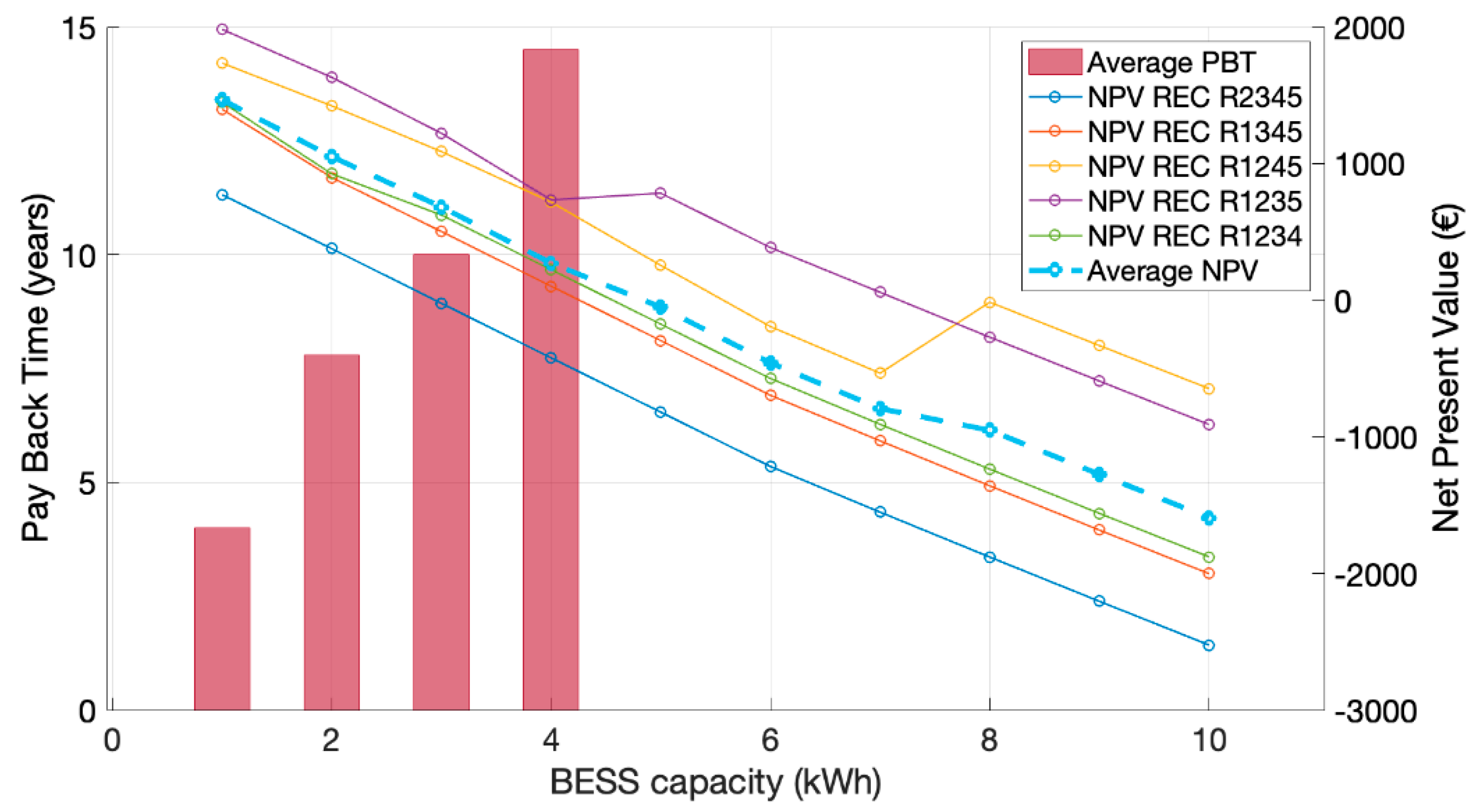
• The optimal BESS sizing analysis carried out for the considered REC, considering net present value over a 20-year investment lifetime as the main target, described as the optimal choice a 1 kWh / 0.5 kW BESS;
• Such finding could be mainly related to the small size of the considered REC on the one hand, and on the other hand to the combination of little price arbitrage possibility on the Italian day-ahead market and high BESS CAPEX.

Further sensitivity analyses could be carried out by to evaluate the impact of higher price spreads on the DAM, together with lower BESS CAPEX, also related to incentivizing policies.

References

1. Nouicer, A.-M.; Kehoe, J.; Nysten, D.; Fouquet, L.; Hancher, L.; Meeus, L. The EU Clean Energy Package; Florence School of Regulation: Firenze, Italy, 2020. [Google Scholar]
2. European Commission. COM (2021) 550 final—“Fit for 55”: Delivering the EU’s 2030 Climate Target on the Way to Climate Neutrality. 2021. Available online: https://ec.europa.eu/clima/citizens/support_en (accessed on 10 October 2021).
3. European Commission. COM (2019) 640 Final—The European Green New Deal. 2019. Available online: https://eur-lex.europa.eu/resource.html?uri=cellar:b828d165-1c22-11ea-8c1f-01aa75ed71a1.0002.02/DOC_1&format=PDF (accessed on 10 October 2021).
4. Council of the European Union. European Parliament. Directive (EU) 2018/2001 on the promotion of the use of energy from renewable sources (recast). Off. J. Eur. Union 2018, 328, 82–209. [Google Scholar]
5. European Parliament. Directive (EU) 2019/944—On common rules for the internal market for electricity and amending Directive 2012/27/EU (recast). Off. J. Eur. Union 2019, 50, 30. Available online: http://eur-lex.europa.eu/pri/en/oj/dat/2003/l_285/l_28520031101en00330037.pdf (accessed on 10 October 2021).
6. Italian Parliament. Law n.8 28/02/2020; Italian Parliament: Rome, Italy, 2020.
7. Ministry for Economic Development. Decreto Ministeriale D.M. 16/09/2020. Off. J. Eur. Union 2020, 285, 37–41. [Google Scholar]
8. ARERA. Deliberazione 4 Agosto 2020 318/2020/R/EEL—Regolazione delle Partite Economiche Relative All’energia Elettrica Condivisa da un Gruppo di Autoconsumatori di Energia Rinnovabile che Agiscono Collettivamente in Edifici e Condomini Oppure Condivisa in una Comunità di Energia Rinnovabile. 2020. Available online: https://www.arera.it/allegati/docs/20/318-20.pdf (accessed on 15 October 2021).
9. Grasso, F.; Abdollahi, M.; Talluri, G.; Paolucci, L. Power control and energy management of grid-scale energy storage systems for smart users. In Proceedings of the 2019 AEIT International Annual Conference (AEIT), Firenze, Italy, 18–20 September 2019. [Google Scholar] [CrossRef]
10. Grasso, F.; Abdollahi, M.; Talluri, G.; Paolucci, L. Techno-economic control of energy storage system for demand side management. In Proceedings of the 2019 AEIT International Annual Conference (AEIT), Firenze, Italy, 18–20 September 2019. [Google Scholar] [CrossRef]
11. Grasso, F.; Talluri, G.; Giorgi, A.; Luchetta, A.; Paolucci, L. Peer-to-peer energy exchanges model to optimize the integration of renewable energy sources: The E-Cube project. Energ. Elettr. Suppl. J. 2019, 96, 1–8. [Google Scholar] [CrossRef]
12. Corti, F.; Gulino, M.-S.; Laschi, M.; Lozito, G.M.; Pugi, L.; Reatti, A.; Vangi, D. Time-domain circuit modelling for hybrid supercapacitors. Energies 2021, 14, 6837. [Google Scholar] [CrossRef]
13. Li, S.; Ju, C.; Li, J.; Fang, R.; Tao, Z.; Li, B.; Zhang, T. State-of-charge estimation of lithium-ion batteries in the battery degradation process based on recurrent neural network. Energies 2021, 14, 306. [Google Scholar] [CrossRef]
14. Li, C.; Xiao, F.; Fan, Y. An approach to state of charge estimation of lithium-ion batteries based on recurrent neural networks with gated recurrent unit. Energies 2019, 12, 1592. [Google Scholar] [CrossRef] [Green Version]
15. Xiao, B.; Liu, Y. Accurate state-of-charge estimation approach for lithium-ion batteries by gated recurrent unit with ensemble optimizer. IEEE Access 2019, 7, 54192–54202. [Google Scholar] [CrossRef]
16. Bonfitto, A. A method for the combined estimation of battery state of charge and state of health based on artificial neural networks. Energies 2020, 13, 2548. [Google Scholar] [CrossRef]
17. Corti, F.; Reatti, A.; Lozito, G.M.; Cardelli, E.; Laudani, A. Influence of non-linearity in losses estimation of magnetic components for DC-DC converters. Energies 2021, 14, 6498. [Google Scholar] [CrossRef]
18. Antonio, S.Q.; Faba, A.; Rimal, H.P.; Cardelli, E. On the analysis of the dynamic energy losses in NGO electrical steels under non-sinusoidal polarization waveforms. IEEE Trans. Magn. 2020, 56, 1–15. [Google Scholar] [CrossRef]
19. Cardelli, E.; Faba, A.; Laudani, A.; Antonio, S.Q.; Fulginei, F.R.; Salvini, A. Computer modeling of nickel–iron alloy in power electronics applications. IEEE Trans. Ind. Electron. 2016, 64, 2494–2501. [Google Scholar] [CrossRef]
20. Henri, G.; Lu, N. A supervised machine learning approach to control energy storage devices. IEEE Trans. Smart Grid 2019, 10, 5910–5919. [Google Scholar] [CrossRef]
21. Gil-González, W.; Montoya, O.D.; Grisales-Noreña, L.F.; Cruz-Peragón, F.; Alcalá, G. economic dispatch of renewable generators and BESS in DC microgrids using second-order cone optimization. Energies 2020, 13, 1703. [Google Scholar] [CrossRef] [Green Version]
22. Cao, B.; Dong, W.; Lv, Z.; Gu, Y.; Singh, S.; Kumar, P. Hybrid microgrid many-objective sizing optimization with fuzzy decision. IEEE Trans. Fuzzy Syst. 2020, 28, 2702–2710. [Google Scholar] [CrossRef]
23. Alramlawi, M.; Li, P. Design optimization of a residential PV-battery microgrid with a detailed battery lifetime estimation model. IEEE Trans. Ind. Appl. 2020, 56, 2020–2030. [Google Scholar] [CrossRef]
24. Qiu, H.; Gu, W.; Xu, Y.; Yu, W.; Pan, G.; Liu, P. Tri-level mixed-integer optimization for two-stage microgrid dispatch with multi-uncertainties. IEEE Trans. Power Syst. 2020, 35, 3636–3647. [Google Scholar] [CrossRef]
25. Montoya, O.D.; Arias-Londoño, A.; Garrido, V.M.; Gil-González, W.; Grisales-Noreña, L.F. A quadratic convex approximation for optimal operation of battery energy storage systems in DC distribution networks. Energy Syst. 2021, 1–21. [Google Scholar] [CrossRef]
26. Sheha, M.; Powell, K. Using real-time electricity prices to leverage electrical energy storage and flexible loads in a smart grid environment utilizing machine learning techniques. Processes 2019, 7, 870. [Google Scholar] [CrossRef] [Green Version]
27. Kong, W.; Dong, Z.Y.; Jia, Y.; Hill, D.J.; Xu, Y.; Zhang, Y. Short-term residential load forecasting based on LSTM recurrent neural network. IEEE Trans. Smart Grid 2017, 10, 841–851. [Google Scholar] [CrossRef]
28. Kong, W.; Dong, Z.Y.; Hill, D.J.; Luo, F.; Xu, Y. Short-term residential load forecasting based on resident behaviour learning. IEEE Trans. Power Syst. 2017, 33, 1087–1088. [Google Scholar] [CrossRef]
29. Tian, C.; Ma, J.; Zhang, C.; Zhan, P. A deep neural network model for short-term load forecast based on long short-term memory network and convolutional neural network. Energies 2018, 11, 3493. [Google Scholar] [CrossRef] [Green Version]
30. Deng, Z.; Wang, B.; Xu, Y.; Xu, T.; Liu, C.; Zhu, Z. Multi-scale convolutional neural network with time-cognition for multi-step short-term load forecasting. IEEE Access 2019, 7, 88058–88071. [Google Scholar] [CrossRef]
31. Sadaei, H.J.; Silva, P.C.D.L.E.; Guimarães, F.G.; Lee, M.H. Short-term load forecasting by using a combined method of convolutional neural networks and fuzzy time series. Energy 2019, 175, 365–377. [Google Scholar] [CrossRef]
32. Garcia, C.I.; Grasso, F.; Luchetta, A.; Piccirilli, M.C.; Paolucci, L.; Talluri, G. A comparison of power quality disturbance detection and classification methods using CNN, LSTM and CNN-LSTM. Appl. Sci. 2020, 10, 6755. [Google Scholar] [CrossRef]
33. Jalali, S.M.J.; Ahmadian, S.; Khosravi, A.; Shafie-Khah, M.; Nahavandi, S.; Catalao, J.P.S. A novel evolutionary-based deep convolutional neural network model for intelligent load forecasting. IEEE Trans. Ind. Inform. 2021, 17, 8243–8253. [Google Scholar] [CrossRef]
34. Li, Y.; Huang, Y.; Zhang, M. Short-term load forecasting for electric vehicle charging station based on niche immunity lion algorithm and convolutional neural network. Energies 2018, 11, 1253. [Google Scholar] [CrossRef] [Green Version]
35. Grasso, F.; Luchetta, A.; Manetti, S. A multi-valued neuron based complex ELM neural network. Neural Process. Lett. 2017, 48, 389–401. [Google Scholar] [CrossRef]
36. Zahid, M.; Ahmed, F.; Javaid, N.; Abbasi, R.A.; Zainab Kazmi, H.S.; Javaid, A.; Bilal, M.; Akbar, M.; Ilahi, M. Electricity price and load forecasting using enhanced convolutional neural network and enhanced support vector regression in smart grids. Electronics 2019, 8, 122. [Google Scholar] [CrossRef] [Green Version]
37. Alanis, A.Y. Electricity prices forecasting using artificial neural networks. IEEE Lat. Am. Trans. 2018, 16, 105–111. [Google Scholar] [CrossRef]
38. Fraunholz, C.; Kraft, E.; Keles, D.; Fichtner, W. Advanced price forecasting in agent-based electricity market simulation. Appl. Energy 2021, 290, 116688. [Google Scholar] [CrossRef]
39. Wang, Z.; Hong, T. Generating realistic building electrical load profiles through the Generative Adversarial Network (GAN). Energy Build. 2020, 224, 110299. [Google Scholar] [CrossRef]
40. Gu, Y.; Chen, Q.; Liu, K.; Xie, L.; Kang, C. GAN-based model for residential load generation considering typical consumption patterns. In Proceedings of the 2019 IEEE Power & Energy Society Innovative Smart Grid Technologies Conference (ISGT), Washington, DC, USA, 18–21 February 2019. [Google Scholar] [CrossRef]
41. Ge, L.; Liao, W.; Wang, S.; Bak-Jensen, B.; Pillai, J.R. Modeling daily load profiles of distribution network for scenario generation using flow-based generative network. IEEE Access 2020, 8, 77587–77597. [Google Scholar] [CrossRef]
42. Pan, Z.; Wang, J.; Liao, W.; Chen, H.; Yuan, D.; Zhu, W.; Fang, X.; Zhu, Z. Data-driven EV load profiles generation using a variational auto-encoder. Energies 2019, 12, 849. [Google Scholar] [CrossRef] [Green Version]
43. Talluri, G.; Grasso, F.; Chiaramonti, D. Is deployment of charging station the barrier to electric vehicle fleet development in EU urban areas? An analytical assessment model for large-scale municipality-level EV charging infrastructures. Appl. Sci. 2019, 9, 4704. [Google Scholar] [CrossRef] [Green Version]
44. Moncecchi, M.; Meneghello, S.; Merlo, M. Energy sharing in renewable energy communities: The Italian case. In Proceedings of the 2020 55th International Universities Power Engineering Conference (UPEC), Turin, Italy, 1–4 September 2020. [Google Scholar] [CrossRef]
45. Verde, S.; Rossetto, N. The Future of Renewable Energy Communities in the EU—An Investigation at the Time of the Clean Energy Package; European University Institute: Florence, Italy, 2020. [Google Scholar] [CrossRef]
46. Barbour, E.; Parra, D.; Awwad, Z.; González, M.C. Community energy storage: A smart choice for the smart grid? Appl. Energy 2018, 212, 489–497. [Google Scholar] [CrossRef] [Green Version]
47. Bartolini, A.; Carducci, F.; Muñoz, C.B.; Comodi, G. Energy storage and multi energy systems in local energy communities with high renewable energy penetration. Renew. Energy 2020, 159, 595–609. [Google Scholar] [CrossRef]
48. Dukovska, I.; Slootweg, H.J.; Paterakis, N.G. Decentralized optimization and power flow analysis for a local energy community. In Proceedings of the 2021 IEEE Madrid PowerTech, Madrid, Spain, 28 June–2 July 2021. [Google Scholar] [CrossRef]
49. Malysz, P.; Sirouspour, S.; Emadi, A. An optimal energy storage control strategy for grid-connected microgrids. IEEE Trans. Smart Grid 2014, 5, 1785–1796. [Google Scholar] [CrossRef]
50. Elkazaz, M.; Sumner, M.; Pholboon, S.; Thomas, D. Microgrid energy management using a two stage rolling horizon technique for controlling an energy storage system. In Proceedings of the 7th International Conference on Renewable Energy Research and Applications (ICRERA), Paris, France, 14–17 October 2018; pp. 324–329. [Google Scholar] [CrossRef]
51. Jung, S.; Yoon, Y.T.; Huh, J.-H. An efficient micro grid optimization theory. Mathematics 2020, 8, 560. [Google Scholar] [CrossRef] [Green Version]
52. Chis, A.; Koivunen, V. Collaborative approach for energy cost minimization in smart grid communities. In Proceedings of the 2017 IEEE Global Conference on Signal and Information Processing (GlobalSIP), Montreal, QC, Canada, 14–6 November 2017. [Google Scholar]
53. Al Skaif, T.; Luna, A.C.; Zapata, M.G.; Guerrero, J.; Bellalta, B. Reputation-based joint scheduling of households appliances and storage in a microgrid with a shared battery. Energy Build. 2017, 138, 228–239. [Google Scholar] [CrossRef] [Green Version]
54. Bandara, K.Y.; Thakur, S.; Breslin, J. Renewable energy integration through coalition formation for P2P energy trading. In Proceedings of the 2020 IEEE 3rd International Conference on Renewable Energy and Power Engineering (REPE), Edmonton, AB, Canada, 9–11 October 2020; pp. 56–60. [Google Scholar] [CrossRef]
55. Cui, S.; Wang, Y.-W.; Li, C.; Xiao, J.-W. Prosumer community: A risk aversion energy sharing model. IEEE Trans. Sustain. Energy 2019, 11, 828–838. [Google Scholar] [CrossRef]
56. Xing, X.; Xie, L.; Meng, H.; Guo, X.; Yue, L.; Guerrero, J.M. Multi-time-scale energy management strategy considering battery operation modes for grid-connected microgrids community. CSEE J. Power Energy Syst. 2019, 6, 1–10. [Google Scholar] [CrossRef]
57. Chaouachi, A.; Kamel, R.M.; Andoulsi, R.; Nagasaka, K. Multiobjective intelligent energy management for a microgrid. IEEE Trans. Ind. Electron. 2013, 60, 1688–1699. [Google Scholar] [CrossRef]
58. Elshurafa, A.M. The value of storage in electricity generation: A qualitative and quantitative review. J. Energy Storage 2020, 32, 101872. [Google Scholar] [CrossRef]
59. Beltran, H.; Ayuso, P.; Pérez, E. Lifetime expectancy of li-ion batteries used for residential solar storage. Energies 2020, 13, 568. [Google Scholar] [CrossRef] [Green Version]
60. d’Halluin, P.; Rossi, R.; Schmela, M. European Market Outlook for Residential Battery Storage 2020–2024. 2020. Available online: https://resource-platform.eu/wp-content/uploads/files/statements/2820-SPE-EU-Residential-Market-Outlook-07-mr.pdf (accessed on 16 October 2021).
61. Koskela, J.; Rautiainen, A.; Järventausta, P. Using electrical energy storage in residential buildings—Sizing of battery and photovoltaic panels based on electricity cost optimization. Appl. Energy 2019, 239, 1175–1189. [Google Scholar] [CrossRef]
62. De Lia, F. Incentivi e Norme di Connessione Degli Impianti Fotovoltaici con Accumulo alla Rete Elettrica—Report RdS/PAR2018/100. 2018. Available online: https://www.enea.it/it/Ricerca_sviluppo/documenti/ricerca-di-sistema-elettrico/adp-mise-enea-2015-2017/accumulo-di-energia/report-2018/rds_par2018_100.pdf (accessed on 18 October 2021).
63. Gestore Mercati Energetici. Database of Day-Ahead Electricity Market Prices. 2021. Available online: https://www.mercatoelettrico.org/it/Statistiche/ME/DatiSintesi.aspx (accessed on 7 November 2021).
64. ARERA. Economic Settlements for Residential Customer—Electricity. 2021. Available online: https://www.arera.it/it/dati/condec.htm (accessed on 7 November 2021).
Figure 1. General architecture of a Renewable Energy Community.
Energies 14 08480 g001
Figure 2. Example of the TSR decomposition on a section of the dataset, 30 days of the Consumer 1 Load Profile decomposed in Trend, Seasonality and Residual.
Energies 14 08480 g002
Figure 3. Seasonal Variance and Mean Squared Residual for different seasonality windows length. Two optimal values where both the variance is high, and the residual is low can be found for 24 h and 48 h.
Energies 14 08480 g003
Figure 4. Example of the correlation matrix between the weather environmental variables and the produced PV power. Diagonal elements show the histogram of the variables, off-diagonal elements show the scatter plot between the variables.
Energies 14 08480 g004
Figure 5. Layer diagram for a layer-recurrent neural network with a single hidden recurrent layer with neurons featuring non-linear activation function.
Energies 14 08480 g005
Figure 6. Decision tree algorithm flowchart.
Energies 14 08480 g006
Figure 7. Extract of the enriched dataset showing forecasts for the PV produced power, the individual consumed power and the REC consumed power with different compositions.
Energies 14 08480 g007
Figure 8. Extract of the BESS charge (positive) and discharge (negative) power curve (black) and corresponding BESS SoC curve (purple) (a); extract of forecasted REC loads (black) and prosumer net load (light blue) and generation (purple) curves (b). On the background of (a,b) the DAM prices. Both (a,b) are related to the same REC configuration and to the same 6-days period.
Energies 14 08480 g008
Figure 9. Extract of the BESS SoC curve (purple) over the same 6-days period for REC R1234 (a) and R2345 (b) configurations.
Energies 14 08480 g009
Figure 10. Three-days extract from real-time BESS management outcomes showing a comparison between real-time operation (light blue) and MILP scheduled setpoints (red) for BESS capacity and usage (a). Comparison between MILP scheduling for average BESS power exchange over hourly time periods (red) and corresponding real-time BESS power exchanges (light blue) (b).
Energies 14 08480 g010
Figure 11. PV energy usage report for the three considered scenario.
Energies 14 08480 g011
Figure 12. NPV (line chart) and PBT (bar chart) for BESS investment in the “BESS, MILP” scenario. The light blue, dashed line refers to the averaged NPV across all the REC configurations, while the solid lines refer to the NPV for one of the five specific REC configuration analyzed.
Energies 14 08480 g012