Numerical Simulation via CFD Methods of Nitrogen Flooding in Carbonate Fractured-Vuggy Reservoirs

Abstract

A reservoir-scale numerical conceptual model was established according to the actual geological characteristics of a carbonate fractured-vuggy reservoir. Considering the difference in density and viscosity of fluids under reservoir conditions, CFD (computational fluid dynamic) porous medium model was applied to simulate the process of nitrogen displacement in a fractured-vuggy reservoir after water flooding. The effects of gas injection rate, injection mode, and injector–producer location relation were studied. The results show that nitrogen flooding can yield additional oil recovery of 7–15% after water flooding. Low-speed nitrogen injection is beneficial in obtaining higher oil recovery. High speed injection can expand the sweep area, but gas channeling occurs more easily. In gas–water mixed injection mode, there is fluid disturbance in the reservoir. The gas channeling is faster in low injector–high producer mode, while the high injector–low producer mode is beneficial for increasing the gas sweep range. Nevertheless, the increment of recovery is closely related to well pattern. After nitrogen flooding, there are still a lot of remaining oil distributed in the trap area of gas cap and bottom water in the reservoir that water and gas injection can’t sweep. The establishment of the numerical conceptual model compensates for the deficiency of physical simulation research, stating that only limited parameters can be simulated during experiments, and provides theoretical bases for nitrogen flooding in fractured-vuggy reservoir.

1. Introduction

In Tahe oilfield (Tarim basin, China), there are a lot of fractured-vuggy carbonate reservoirs with depths of 5320–6200 m. This type of reservoir is mainly composed of paleokarst cave, dissolution cave, and fracture with different sizes and shapes, which is essentially different from the traditional sandstone reservoir and fractured porous carbonate reservoir [1]. The reservoir is highly heterogeneous [2] and fluid flow mode is mainly pipe flow [3]. In the early-stage development of these fractured-vuggy reservoirs, water drive was the main development method. The injected water and natural bottom water channeling occur fast along high-angle fractures. For water drive development in fractured-vuggy reservoirs, formation energy depletion is obvious. Gas injection can effectively supplement formation energy and enhance oil recovery. The macroscopic mechanism of nitrogen injection (such as nitrogen huff and puff and nitrogen flooding) in fractured-vuggy reservoir is gravity displacement, caused by density difference, and the microscopic mechanism is that nitrogen can dissolve, expand, and extract with crude oil under conditions of high temperature and high pressure in the reservoir [4,5].

To study the mechanism and oil displacement characteristics of nitrogen flooding, a visual fractured-vuggy model was built and used for simulating displacement experiments of nitrogen flooding [4,6,7,8,9]. The related experimental results show that nitrogen injection time, injection rate, and injection mode have an important impact on oil recovery. Moreover, the relative location of gas injection well and production well also significantly affect the oil recovery, and it was shown that an injection well located at a high position and a production well located at a low position may have a higher oil recovery rate in fractured-vuggy reservoir [5]. The gas injection rate strongly determined the gas channeling characteristics of nitrogen flooding. A too high injection rate can cause an earlier gas breakthrough and lead to a lower enhanced oil recovery [10,11,12,13]. The gas–water synergy and bottom water energy are also found to be important factors affecting gas channeling. Usually, foam can be used to effectively control gas flow rate and delay gas channeling. The local sweep efficiency is determined by the structure of fracture and caves in fractured-vuggy reservoirs. Some residual oil still exists after nitrogen flooding. For example, there are residual oils in the middle of karst cave due to gas channeling and insufficient energy of bottom water, as well as oil film and small oil slug remains in fractures, due to the low efficiency of gas flushing [4]. Visual physical simulation can intuitively show the process of nitrogen flooding. However, it failed to simulate the severe reservoir conditions, including high temperature (120 °C), high pressure (60 MPa), and gas–liquid density difference, etc., due to the limitation of model materials (such as acrylic or glass), size, and production process.

Numerical simulation is an effective method for solving the aforementioned problems of physical simulation. The previous numerical simulation of fractured-vuggy reservoir is based on the theory of multiple continuous media [14], that is, the conventional simulation method of classic reservoir (black oil model). In this way, the flow in caves and fractures is assumed to be Darcy flow. In fact, the flow in the large-scale fractures or caves includes the seepage flow in the boundary of micro fractures and caves and the free flow in the large-scale fractures and caves. Based on the pseudo particle method, a multi-scale discrete calculation model [15] of oil–water two-phase flow was established to simulate the flow in fractured-vuggy reservoirs. If only focusing on the macroscopic flow law of fluid, the flow model of fractured-vuggy reservoir can be simplified and three-dimensional problems can be transformed into two-dimensional ones; thus, the fluid flow can be considered as pipe flow [16].Therefore, the equivalent simulation method of large-scale fractured-vuggy body was proposed [17,18]. The improved equivalent continuum model (ECM) was used to simulate micro fractures and dissolved pores, while the embedded discrete fracture model (EDFM) and unmatched mesh were used for the explicit modeling of macro fractures and caves [19]. Based on the aforementioned modeling methods, a numerical simulation software for fractured-vuggy reservoir was developed [20,21,22].

For nitrogen flooding in fractured-vuggy reservoirs, the main focuses are oil recovery factor, macro-scale flow, and fluid distribution characteristics. Therefore, in the reservoir scale, the influence of micro seepage on nitrogen flooding can be ignored, and nitrogen flow in reservoir scale can be considered as a macro-free flow. Computational fluid dynamic (CFD) is a widely used method to simulate free flow in petroleum industry [23,24,25]. For instance, in drilling stage, the concentration of drilling cuttings in drill pipe annulus can be used as the main parameter to evaluate well flushing efficiency [26], and the size of stable water plugging nanoparticles in shale wellbore can be determined through CFD-DEM simulation [27]. CFD model can be established to study the effect of wellbore shape on gas well production efficiency [28], and it can be also used to study the flow dynamic of intermittent gas lift valve [29,30]. A CFD and VOF (volume of fluid) coupling model is used to simulate the flow in a single fracture–cavity unit, and the oil–water interface can be tracked [31].CFD method is also used to study the influence of pore-scale viscous fingering [32] and formation water composition on the recovery in carbonate reservoir [33]. CFD and Hernandez models are coupled to simulate and quantitatively characterize the distribution of residual oil in fractured-vuggy reservoir [34]. For the calculation of the numerical model, based on the traditional pore media models, including continuous models, lattice Boltzmann models, and discrete structure network models [35], a PIML workflow [36,37] for unconventional reservoirs (shale gas reservoirs) was proposed, which can quickly and accurately fit the production process of shale gas reservoirs and make a prediction.

In this work, a reservoir scale numerical conceptual model was established, based on the geological characteristics of a real fractured-vuggy reservoir in Tahe oilfield. Based on CFD method, the numerical simulation of nitrogen flooding in fractured-vuggy reservoir was carried out and the factors, such as nitrogen injection rate, injection mode, and injection–production relation, etc., affecting the recovery of nitrogen flooding, were systematically studied.

2. Numerical Model

2.1. Model Simplification and Simulation Conditions

The seismic interpretation results show that well group TK411-TK401 in Tahe oilfield has the karst geological structure of a weathering crust at the top and an underground river at the bottom (Figure 1). Based on the morphological characteristics of weathering crusts and underground rivers in the karst area (Figure 2), a conceptual model was established (Figure 3) which has a total volume of 202,840 m³.

In the numerical model, the boundary conditions of the injection well are the mass flow inlet, bottom water inlet is the pressure inlet, and the boundary condition of production well is the pressure outlet. To simulate the heterogeneity of the reservoir, different filling degrees were set in Figure 3. The filling degree gradually increases from top to bottom, and the filling degree of fractures and bottom of wellbore is the same. The dimensions represented by the numerical model are also shown in Figure 3. Using this model, natural water flooding (bottom water flooding), artificial water injection, and nitrogen flooding were simulated. The simulation scheme includes the following steps:

• 3D modeling of fracture-vuggy structure.

According to the interpretation results of reservoir seismic data, the 3D fracture-vuggy structure diagram was drawn in proportion.

• Initial oil–water distribution simulation.

The initial oil–water distribution in the karst structure in TK411-T401 well group, under the effect of gravity, was simulated. The parameters involved in the simulation are shown in

Table 1. Simulation parameters (reservoir condition).

Pressure (MPa)	Oil Viscosity (MPa·s)	Oil Density (g/cm3)	Brine Viscosity (MPa·s)	Brine Density (g/cm3)
60	30	0.80	0.20	1.13

.

• Natural water flooding.

The simulation of natural water flooding (bottom water) was carried out under the condition of original oil–water distribution. The process of infinite bottom water (60 MPa) flooding to water cut of 98% or higher was simulated.

• Artificial water flooding simulation.

After natural water flooding to a water cut of 98%, water injection wells were set in the lower part of the reservoir for artificial water injection, and the infinite bottom water pressure (60 MPa) remained unchanged. The water injection rate in the oil field was 200 ~ 500 m³/d, and the artificial water injection of 300 m³/d was used for simulation.

• Nitrogen flooding simulation.

After the above steps were completed, the nitrogen flooding from the injection well was simulated. By setting nitrogen injection rate, nitrogen injection mode, and changing the injection well position, the nitrogen flooding under different conditions can be simulated.

2.2. Numerical Method

2.2.1. Assumptions

The assumptions for building this model were the following: (1) the flow in fractured-vuggy reservoirs is laminar flow; (2) the porosity in the reservoir is isotropic; (3) the fluid medium is incompressible; (4) the reservoir temperature is stable; and (5) the physical properties of fluid in the reservoir are estimated by the given density and viscosity values.

2.2.2. Governing Equations

The porous medium model was applied, which can be used to study single-phase flow and multiphase flow. It is necessary to determine the pressure loss in the flow when using the porous medium model. The pressure loss was calculated by the momentum equation (Equation (1)). In order to simplify the simulation, the fluid was considered as viscous incompressible, and the energy equation in porous medium is ignored. In view of the influence of the compressible fluid and temperature on the fluid properties in the reservoir, the reservoir conditions were approximated by the given viscosity and density values.

$$S_i=-\left({{\displaystyle \sum }}_{j=1}^3{D}_{ij}\mu v_j+{{\displaystyle \sum }}_{j=1}^3{C}_{ij}\frac{1}{2}\rho \left|v\right|v_j\right)$$

(1)

where $S_i$ is the source term of the ith ($\mathrm{X},\mathrm{Y}$, or $\mathrm{Z}$ axis direction) momentum equation;$\left|v\right|$ is the amplitude of the velocity; $D_{ij}$ and $C_{IJ}$ are specified matrices; $i$ and $j$ are serial numbers. Equation (1) consists of two parts: a viscous loss part and an inertial loss part, which are the first and second part are at the right part of Equation (1), respectively. The negative source term is also known as “sink”. The contribution of momentum sink to the momentum gradient of porous medium element produces a pressure drop proportional to the fluid velocity (or velocity Square).

The following mathematical models (Equation (2)) can also be used for simplified and homogeneous porous medium:

$$S_i=-\left(\frac{\mu }{\alpha }{v}_i+C_2\frac{1}{2}\rho \left|v\right|v_i\right)$$

(2)

where α is the permeability of porous medium and $C_2$ is the inertial drag factor. D and C in Equation (1) are defined as diagonal matrices with 1⁄α and $C_2$ is a diagonal element.

2.2.3. Darcy Law in Porous Medium

Since the flow in fractured-vuggy reservoir can be approximately considered as laminar flow, the pressure drop ratio is proportional to the velocity, and the constant $C_2$ in Equation (2) is considered as zero. Neglecting the convection and diffusion terms, the pressure loss equation in the porous medium model is simplified to the following Darcy equation:

$$\nabla p=-\frac{\mu }{\alpha }\overrightarrow{v}$$

(3)

Then, the pressure drop calculated in X, Y, and Z coordinates are as follows:

$$\Delta p_x={{\displaystyle \sum }}_{j=1}^3\frac{\mu }{{\alpha }_{xj}}{v}_j\Delta n_x$$

(4)

$$\Delta p_y={{\displaystyle \sum }}_{j=1}^3\frac{\mu }{{\alpha }_{yj}}{v}_j\Delta n_y$$

(5)

$$\Delta p_z={{\displaystyle \sum }}_{j=1}^3\frac{\mu }{{\alpha }_{zj}}{v}_j\Delta n_z$$

(6)

where $\frac{1}{{\alpha }_{ij}}$ is $\mathrm{D}$ in Equation (1),$v_j$ is the velocity component in X, Y, and Z coordinates, and $\Delta n_x$, $\Delta n_y$, $\Delta n_z$ are the true thicknesses of porous mediums in X, Y and Z coordinates, respectively.

2.2.4. Governing Equations of Porous Medium in Multiphase Field

For water injection and nitrogen flooding process in fractured-vuggy reservoirs, to simulate the multiphase flow under reservoir conditions, the physical velocity in porous medium equation was applied. It was assumed that there was a general scalar ${\varphi }_q$ in $qth$, and the governing equation in isotropic porous medium can be expressed as Equation (7):

$$\frac{\partial \left(\gamma {\alpha }_q{\rho }_q{\varphi }_q\right)}{\partial t}+\nabla \left(\gamma {\alpha }_q{\rho }_q\overrightarrow{v_q}{\varphi }_q\right)=\nabla \left(\gamma {\mathsf{\Gamma }}_q\nabla {\varphi }_q\right)+\gamma S_{\varphi ,q}$$

(7)

where $\gamma$ is porosity, ${\rho }_q$ is phase density, ${\alpha }_q$ is volume fraction, $\overrightarrow{v_q}$ is phase velocity vector, $S_{\varphi ,q}$ is the source term, and ${\mathsf{\Gamma }}_q$ is diffusion coefficient. Assuming that all directions have the same porosity and multiphase flow, the governing equations for $qth$ are as follows:

Continuity equation:

$$\frac{\partial }{\partial t}\left(\gamma {\alpha }_q{\rho }_q\right)+\nabla \left(\gamma {\alpha }_q{\rho }_q\overrightarrow{v_q}\right)=\gamma {{\displaystyle \sum }}_{p=1,p\ne q}^n\left({\dot{m}}_{pq}-{\dot{m}}_{qp}\right)+\gamma S_q$$

(8)

Momentum equation:

$$\begin{array}{cc}\hfill \frac{\partial }{\partial t}\left(\gamma {\alpha }_q{\rho }_q{\overrightarrow{v}}_q\right)+\nabla \cdot \left(\gamma {\alpha }_q{\rho }_q{\overrightarrow{v}}_q{\overrightarrow{v}}_q\right)& =-\gamma {\alpha }_q\nabla \left(p-p_c\right)+\nabla \cdot \left(\gamma {\stackrel{=}{\tau }}_q\right)+\gamma {\alpha }_q{\rho }_q{\overrightarrow{B}}_f-\left({\alpha }_q^2{\gamma }^2\frac{{\mu }_q{\overrightarrow{v}}_q}{K{K}_{r,q}}+{\alpha }_q^3{\gamma }^3\frac{c_2{\rho }_q\left|{\overrightarrow{v}}_q\right|{\overrightarrow{v}}_q}{2}\right)\hfill \\ \hfill & +\gamma {{\displaystyle \sum }}_{p=1}^n\left({\overrightarrow{F}}_{pq}^D+{\overrightarrow{F}}_{pq}^{TD}+{\dot{m}}_{pq}{\overrightarrow{v}}_{pq}-{\dot{m}}_{qp}{\overrightarrow{v}}_{qp}\right)+\gamma \left({\overrightarrow{F}}_q+{\overrightarrow{F}}_q^L+{\overrightarrow{F}}_q^{vm}\right)\hfill \end{array}$$

(9)

where $p_c$ is the capillary pressure of the wetting phase, ${\stackrel{=}{\tau }}_q$ is the phase shear stress, ${\overrightarrow{B}}_f$ is the volume force, ${\dot{m}}_{pq}$ is the mass transfer from phase p to phase q, ${\dot{m}}_{qp}$ is mass transfer from phase q to phase p, K is absolute permeability, $K_{r,q}$ is relative permeability, ${\overrightarrow{F}}_{pq}^D$ is the resistance in the non multi-space region, ${\overrightarrow{F}}_{pq}^{TD}$ is the turbulent dissipation force, ${\overrightarrow{v}}_{pq}$ and ${\overrightarrow{v}}_{qp}$ are relative velocity vectors, and ${\overrightarrow{F}}_q$, ${\overrightarrow{F}}_q^L$, and ${\overrightarrow{F}}_q^{vm}$ are external volume force, lift force, and virtual mass exchange force, respectively. Since the compressible and temperature conditions are not involved, the energy equation is negligible.

3. Results and Discussion

3.1. Original Oil–Water Distribution

The original oil distribution in fractured-vuggy reservoir models, obtained by numerical simulation, is shown in Figure 4. Red indicates crude oil and light blue indicates formation water (bottom water). Crude oil and original water exist in the fractures and caves. Because of gravity differentiation, crude oil was originally distributed in the middle and upper parts and water was distributed in lower parts in each fracture–cavity structure.

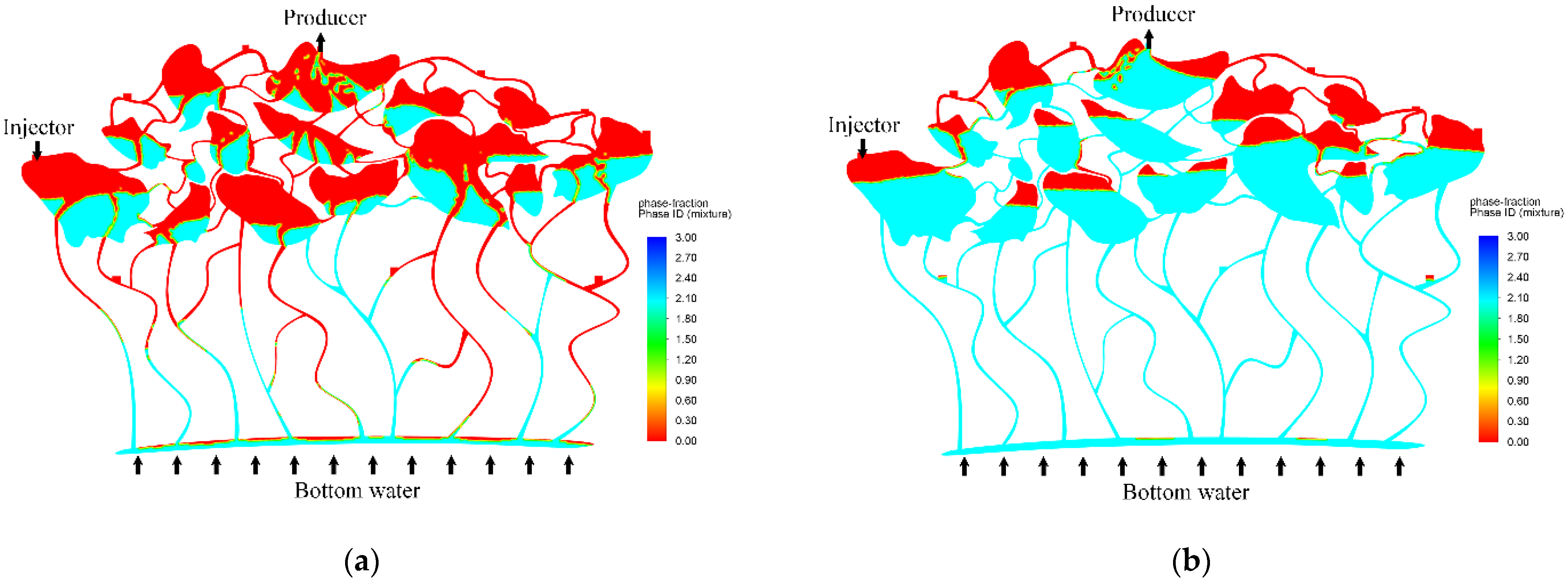
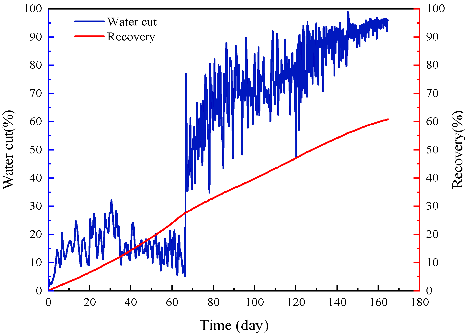
3.2. Natural Water Flooding

The oil–water distribution, in the process of natural water flooding (bottom water flooding), is shown in Figure 5. It can be seen that natural energy (bottom water) displacement can effectively displace oil in fractured-vuggy reservoir.

The oil–water interface in the fracture–cavity structure was uplifted. When the interface arrives at the bottomhole of the production well, a water cone was formed. The remaining oils were left in the higher parts of each structure, like in “attics”. The water cut and cumulative recovery in production wells were monitored during natural water flooding, as shown in Figure 6.

In the initial stage of production, a low water cut was maintained. After the bottom water breaks through to the production well, water cut increased rapidly. Nevertheless, the production rate of oil maintained, as in the initial time, for about 170 days. Under the simulated reservoir pressure of 60 MPa, the recovery of bottom water flooding was 60.8%.

3.3. Artificial Water Injection

Artificial water injection was simulated after natural water flooding under 60 MPa until water cut exceeds 98%, as shown in Figure 7. Water injection rate was 300 m³/d.

It can be observed that the injected water in the middle and lower parts of the model migrated downwards under the action of gravity, and the lateral movement also occurred under the resistance of the bottom water. In this process, the remaining oil flowed together with water to the production well, the injected water wave expanded to other fracture–cavity structure (Figure 7 right, dark blue zone), and an oil–water interface, distributed along the connection line of injection and production wells, was gradually formed [9]. At the end of water injection, the remaining oils were mainly distributed in the higher part of the structures. The water cut curve showed the characteristics of first decreasing followed by increasing (Figure 8). This was expected, as water injection swept some new zones and displaced some remaining oil in the initial stage, while water channeling occurred in the middle and late stages of water injection, making the water cut increase again. The ultimate recovery was 73.21%, and the recovery increment was 12.4% by water injection.

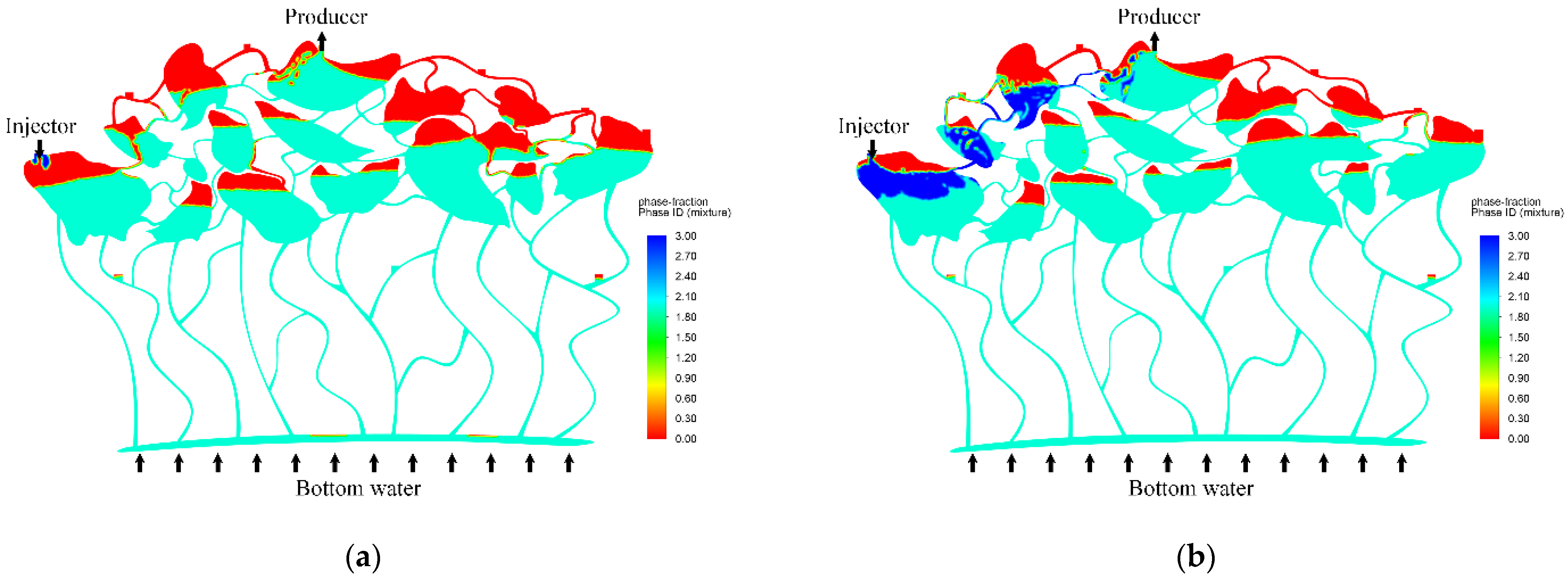
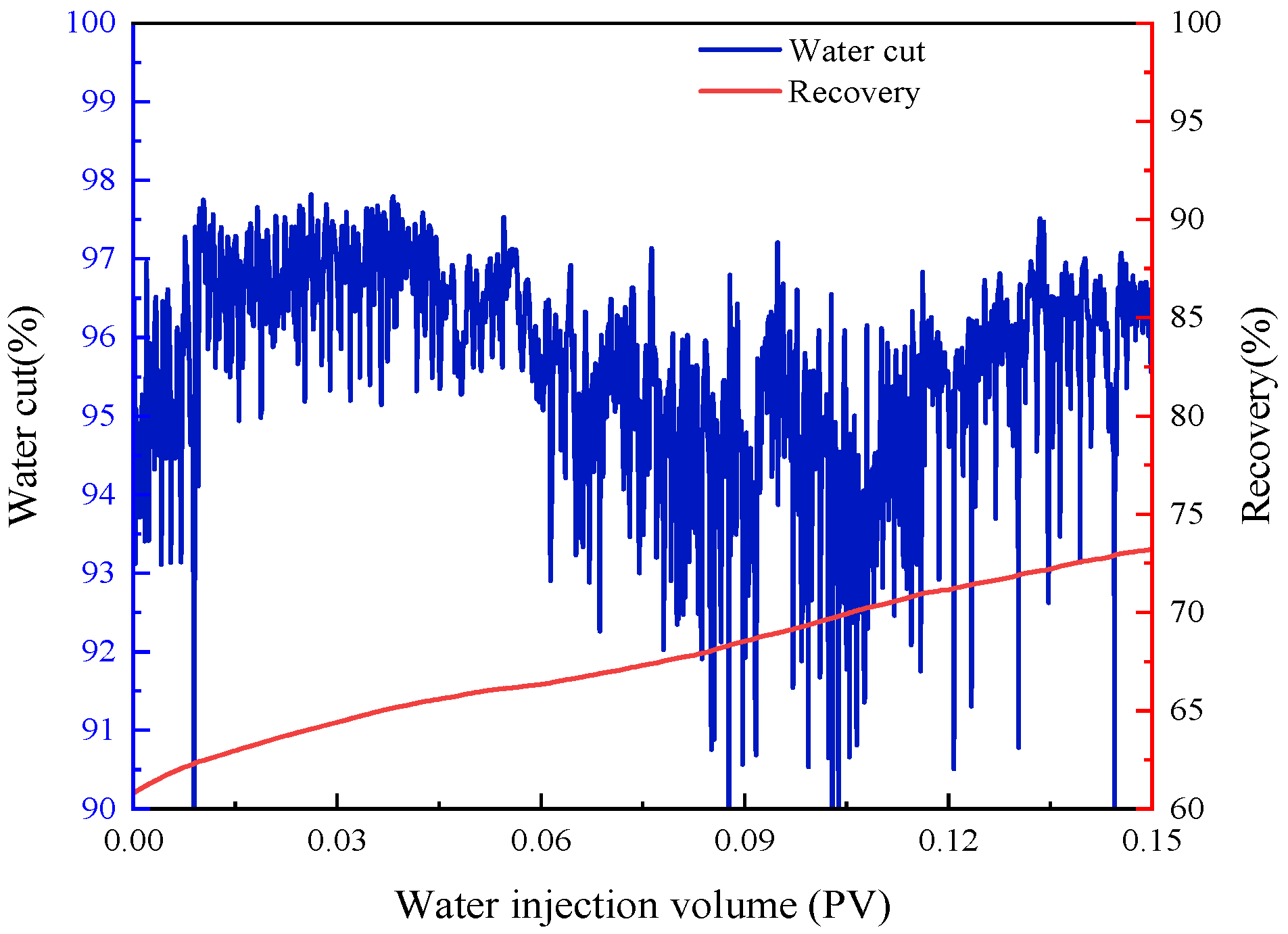
3.4. Nitrogen Flooding

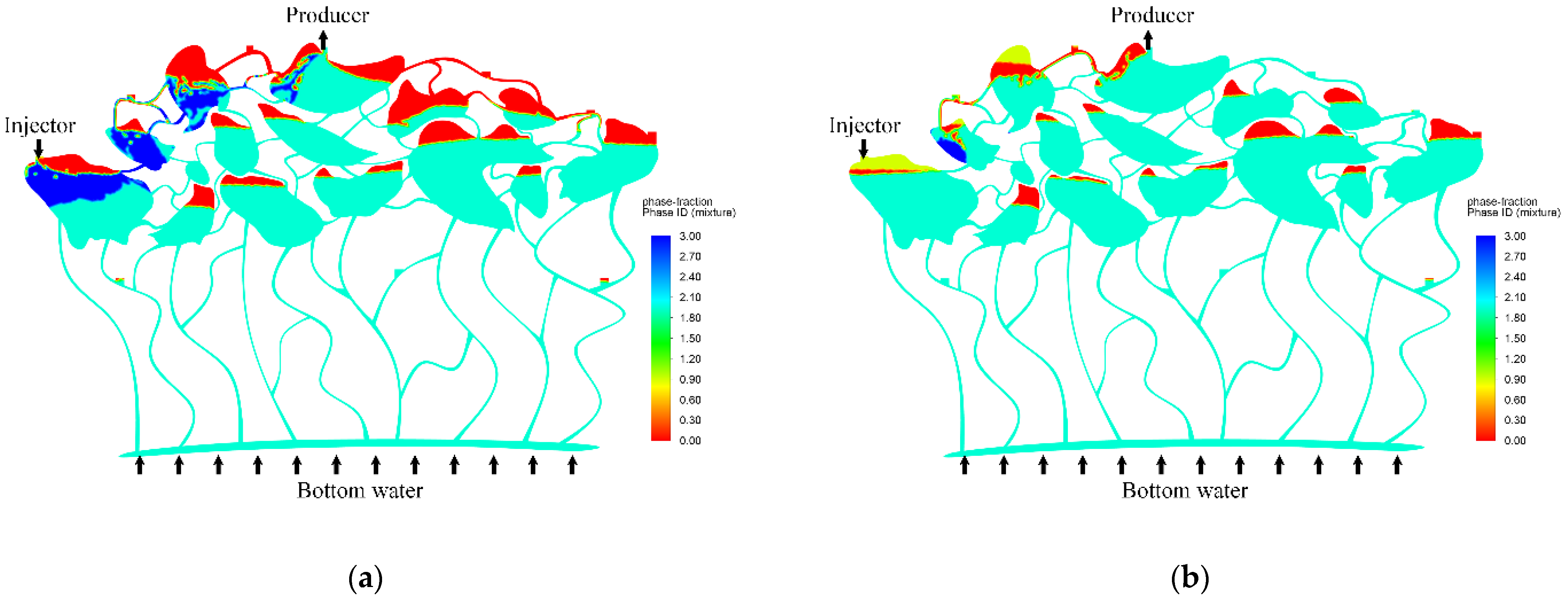
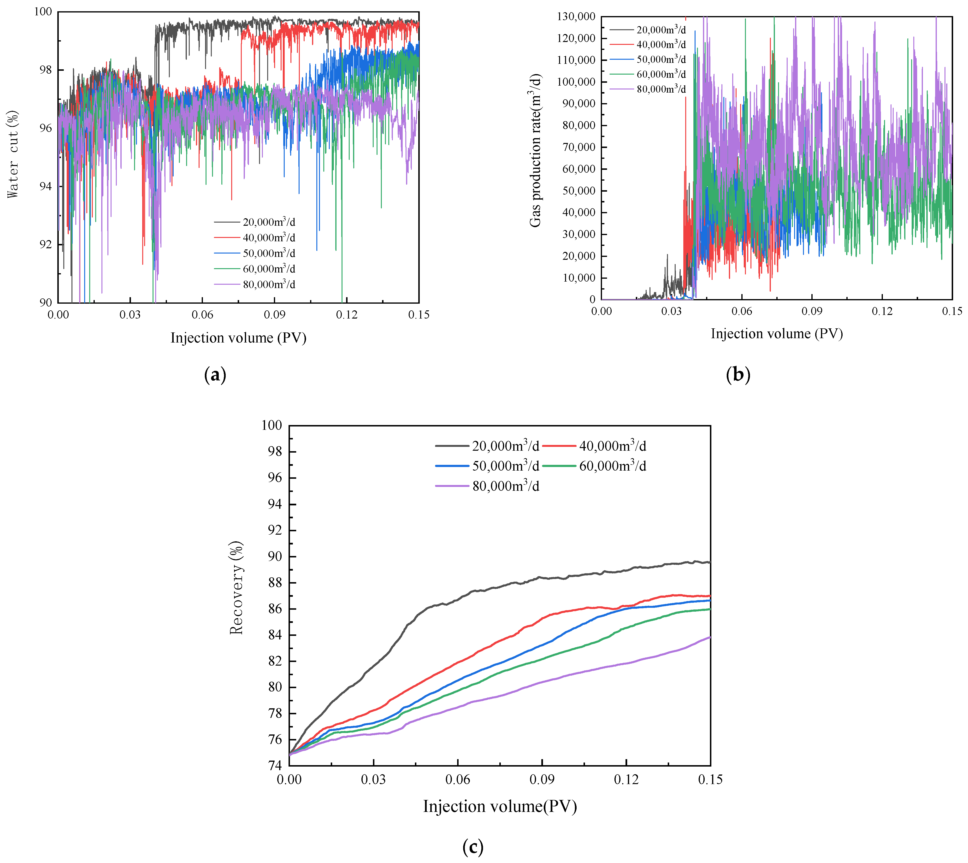
3.4.1. Effect of Injection Flow Rate

After water injection, under the same well pattern, nitrogen injection was carried out at different injection rates (ground condition, 20,000, 40,000, 50,000, 60,000, and 80,000 m³/d). The fluid distribution in fractured-vuggy reservoirs before nitrogen injection (the end of water flooding stage) are the same as Figure 9a shows. Nitrogen injection with different flow (20,000, 40,000, and 80,000 m³/d) resulted different fluid distribution at the end, as Figure 9b–d show (yellow indicates N₂ in the figure).

It can be observed that the injected nitrogen effectively displaces the remaining oil at the higher parts of fractured cavity structures, towards to the production well. In addition to the main channels of water in water injection process, there were several secondary channels for nitrogen flow between injection well and production well. Once the injected nitrogen breaks the overflow point of each fractured cavity structure, parts of the remaining oils are trapped between the gas and bottom water. Moreover, it can be observed that the direction of bottom water flow changed upon nitrogen injection, resulting in the synergistic effect of gas and water [10]. This consequently drove the remaining oil in the non-swept zone during water injection and expanded the swept area of bottom water. After nitrogen flooding, the remaining oil between injection and production wells was mainly distributed in the traps formed by gas and water between wells, in accordance with the finding reported by Lyu X et al. [5].

During nitrogen flooding, water cut, gas production rate, and oil recovery curves monitored in production wells are shown in Figure 10 a–c, respectively. The water cut is decreased when nitrogen injection starts. During the whole nitrogen injection, the water cut curves at different injection rates show “step-like” characteristics. This is because the oil displacement remains stable before the injected gas broke through in the large fracture–vuggy body. When gas channeling occurred, the oil displacement efficiency decreased, and the water cut increased rapidly. The water cut curves, corresponding to the first step, were mainly between 94 and 98%, and the maximum decreasing rate can reach to 8%. The range of water cut, corresponding to the second step, was between 98 and 100%. The higher the injection rate, the later the second step appeared. At the first step, on the one hand, the injected nitrogen drove the remaining oil to the production well, which made the water cut decrease. On the other hand, due to the continuous supplement of bottom water, the water cut rose rapidly, forming a fluctuating water cut curve. At the second step, the swept range of injected nitrogen barely changed. In general, the fluctuation was because the produced gas was disturbed at the bottom of the well, resulting in a large fluctuation of liquid production.

As shown in Figure 10b, when the injection rate was 20,000 m³/d, the injection pore volume (PV) corresponding to gas breakthrough was the smallest (0.02 PV). After gas breakthrough, the well maintained a low production rate for a long period, and the gas production rate reached the peak at about 0.035 PV. Interestingly, the corresponding PV of gas breakthrough at flow rates of 40,000 and 50,000 m³/d increased (in middle level). When the injection rates rose to 60,000 and 80,000 m³/d, gas breakthrough occurred at a larger injection PV, and channeling occurred faster after gas breakthrough [12]. The reason was that the injected gas mainly flowed along the highly permeable part between injector and producer at low injection rate, and the flow path was single. While at high flow rate, multiple flow paths were formed between injector and producer, and the swept area expanded (including water area), thus nitrogen breakthrough occurred at a larger injection PV.

The cumulative recovery curves at different injection flow rates are shown in Figure 10c. The increment of the oil recovery at different injection rates are shown in

Table 2. Recovery increment under different injection rates.

Injection Rate (m3/d)	Cumulative Recovery	Recovery Increment
20,000	89.94%	15.14%
40,000	87.59%	12.79%
50,000	87.24%	12.44%
60,000	86.84%	12.04%
80,000	85.84%	11.04%

. The simulation results showed that a low flow rate of nitrogen injection is beneficial to obtain higher oil recovery, but the injection time of injection flooding may last for a long time in field application. High flow rate can expand the sweep range, but gas channeling may form faster after gas breakthrough due to the fact that new swept areas are usually located at the water bearing area, which causes the recovery increment increase to be relatively low. Considering the operation time and recovery increment in the TK411-T401 well block, the nitrogen injection rate of 40,000–50,000 m³/d is suitable.

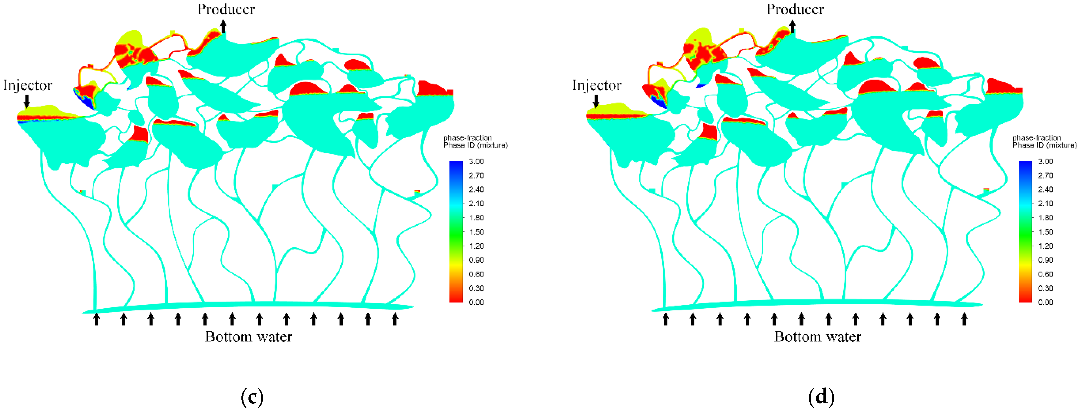
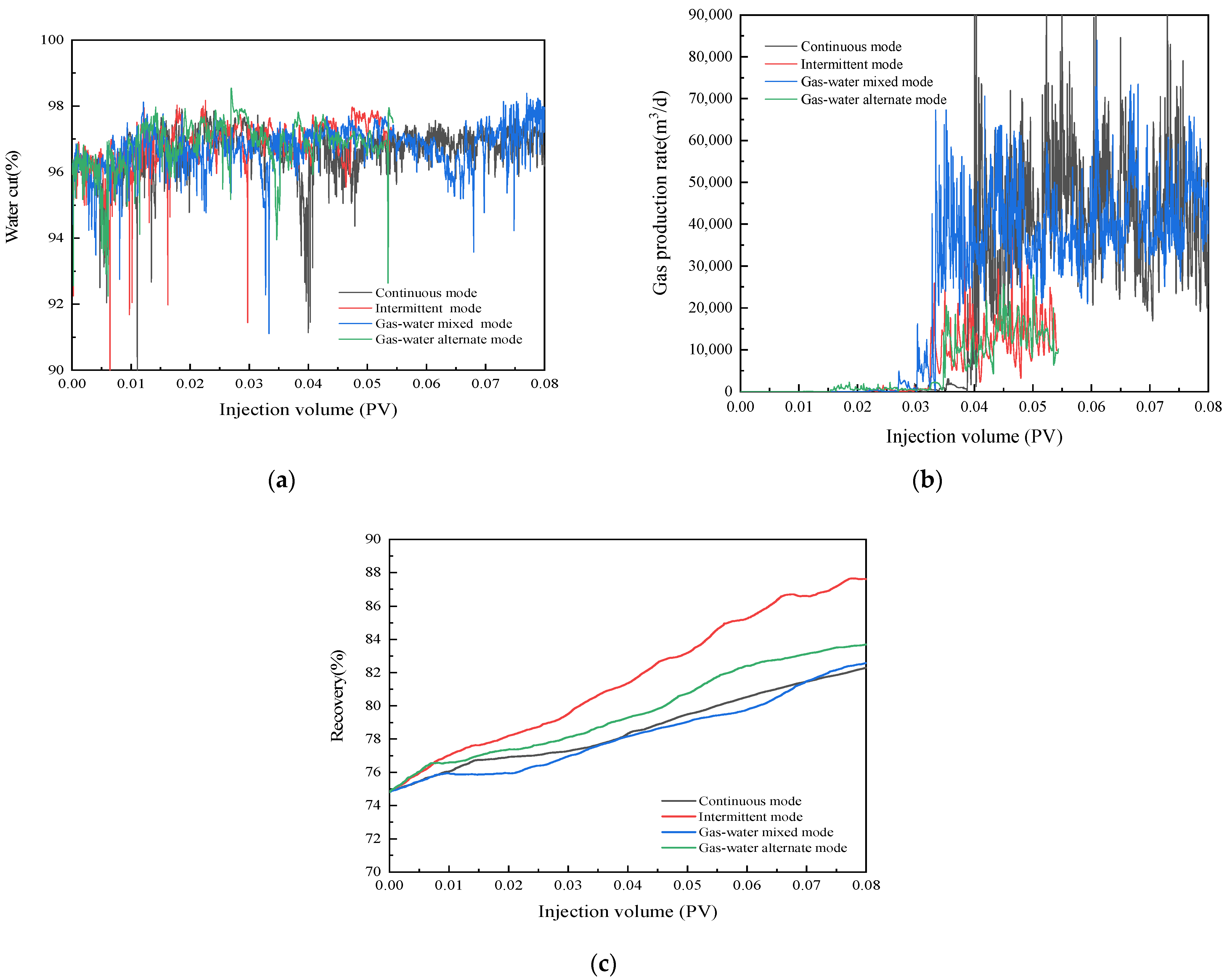
3.4.2. Effect of Injection Mode

After the water flooding (as shown in Figure 11a), the simulation changed to nitrogen flooding with a different injection mode. The oil–water distribution under different nitrogen injection modes, such as continuous mode, intermittent mode, gas–water mixed injection mode, and gas–water alternation mode, were simulated and compared, as shown in Figure 9c and Figure 11b–d. The nitrogen injection PV is 0.05 PV at the injection rate of 50,000 m³/d.

• Continuous mode.

As shown in Figure 9c, the injected gas first entered the high part in the fracture–cavity structure where the injection well is located, and gradually replaced the “attic oil” from the top. With the increase of gas injection, the injected gas flowed from the overflow point along the channel to displace remaining oil to the production well. The injection gas flow formed multiple flow channels. Finally, the remaining oil after nitrogen flooding was trapped between the top gas and bottom water.

• Intermittent mode.

As shown in Figure 11b, the flow characteristics of injected gas and the mobilization of the remaining oil were similar to the continuous mode. The difference was that the injected gas could also replace the “attic oil” during intermittent stop injection, thus delaying the gas channeling.

• Gas–water mixed injection mode.

As shown, near the injection well, the injected gas–water mixture squeezed the remaining oil to the lower area of the fracture–cavity structure, as shown in Figure 11c. The breakthrough of the injected gas–water mixture from the top of the remaining oil to form a flow channel to the production well. Finally, the remaining oil was trapped by gas cap and bottom water near the injection well.

• Gas–water alternate mode.

In the process of gas–water alternate injection (each cycle 15 days), the gas first entered the high point in the fracture–cavity structure where the injection well was located to replace the ‘attic oil’ on the top. In the stage of alternating water injection, the injected water mainly broke through the barrier of the remaining oil by gravity differentiation and flowed downwards toward the bottom of the well. Part of the injected water flowed along the top of the remaining oil to the direction of the production well, and finally formed the oil–water distribution, as shown in Figure 11d.

The curves of water cut, gas production rate, and oil recovery monitored in production wells are shown in Figure 12a–c, respectively. The alternative gas–water injection mode resulted in gas breakthrough at smallest injection PV, followed by intermittent gas injection mode. The breakthrough times of continuous gas injection and gas–water mixed injection were similar, but the gas production rate of gas–water mixed injection mode was lower than that of continuous mode. Compared with the other three gas injection modes, the water cut in the whole process of gas–water mixed injection was the lowest. The reason may be attributed to the injected water, which formed an effective supplement to the bottom water and had a better inhibition effect on the gas production. After injecting the same volume of nitrogen, the recovery increment for different injection modes is shown in

Table 3. Recovery increments of different injection modes.

Injection Mode	Cumulative Recovery	Recovery Increment
Continuous	82.29%	7.49%
Intermittent	87.61%	12.81%
Gas–water mixed	82.58%	7.78%
Gas–water alternate	83.69%	8.89%

. The recovery increment was in the following order: intermittent injection > gas–water alternating injection > gas–water mixed injection > continuous injection. Unstable gas injection mode (intermittent injection and gas–water alternation) can replace the remaining oil under reservoir conditions more efficiently without considering the time cost and operation cost [8]. On the contrary, continuous gas injection (including gas–water mixed injection and continuous gas injection) is not conducive to the diffusion of gas and its displacement efficiency in reservoir.

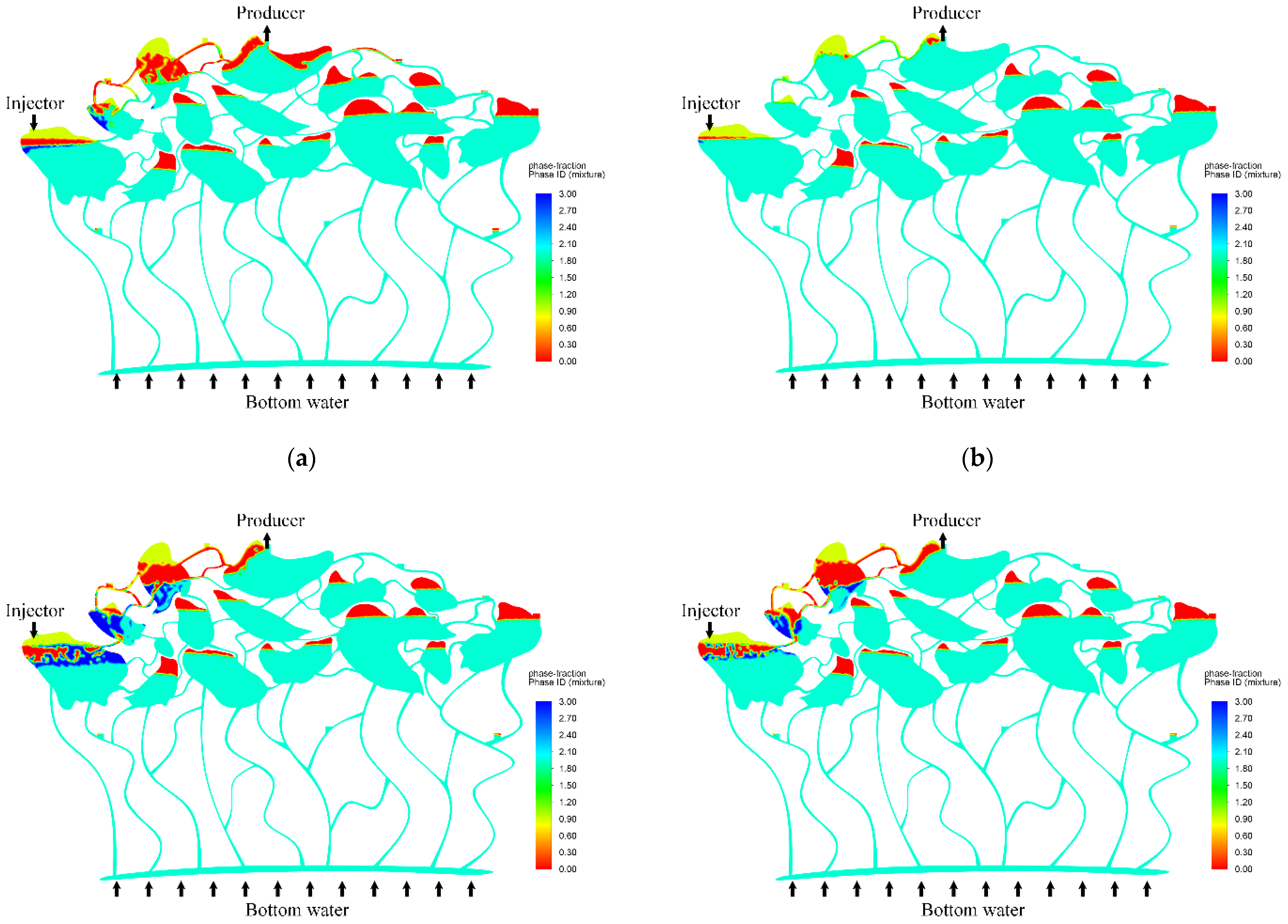
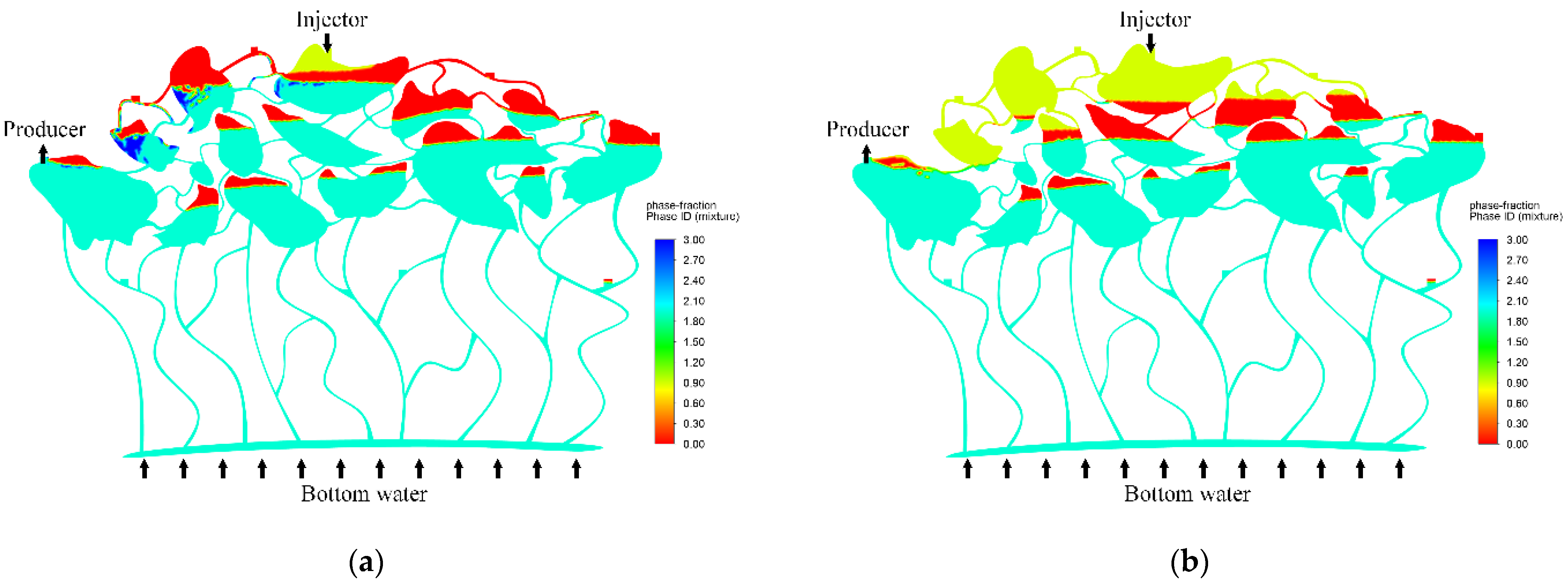
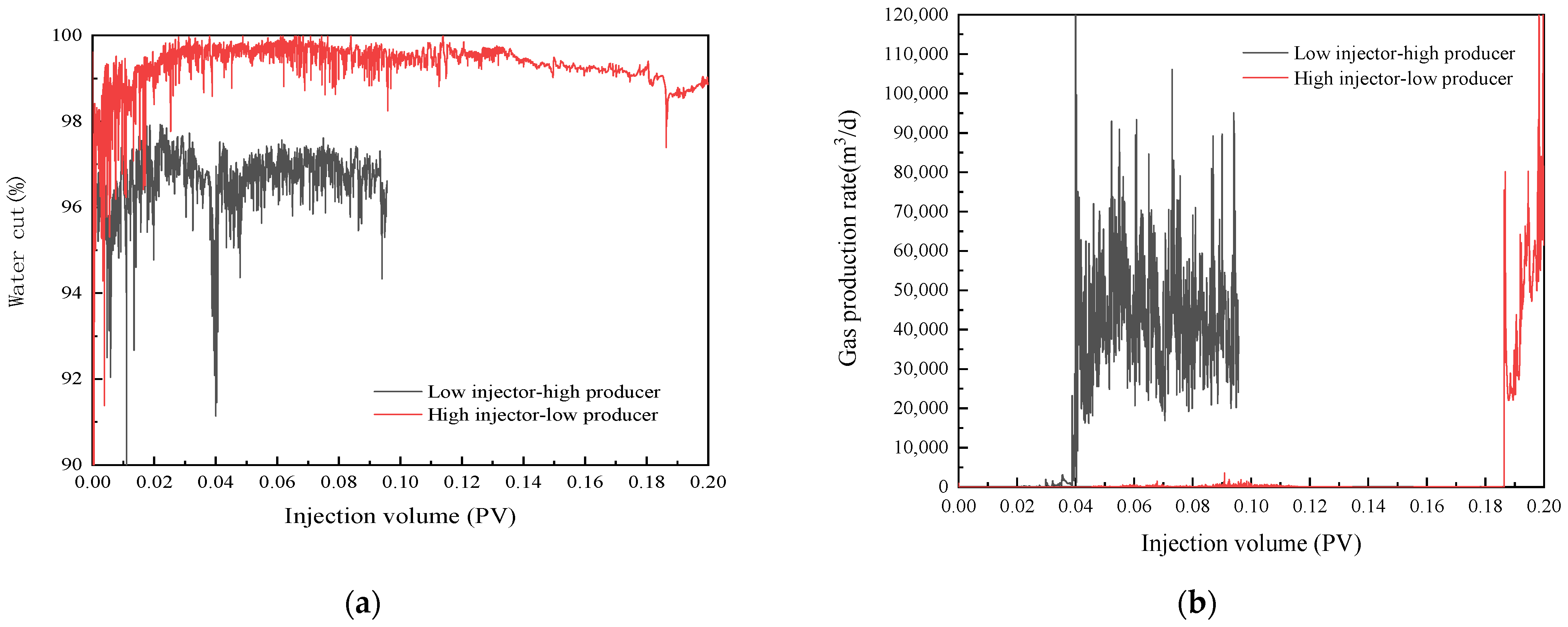
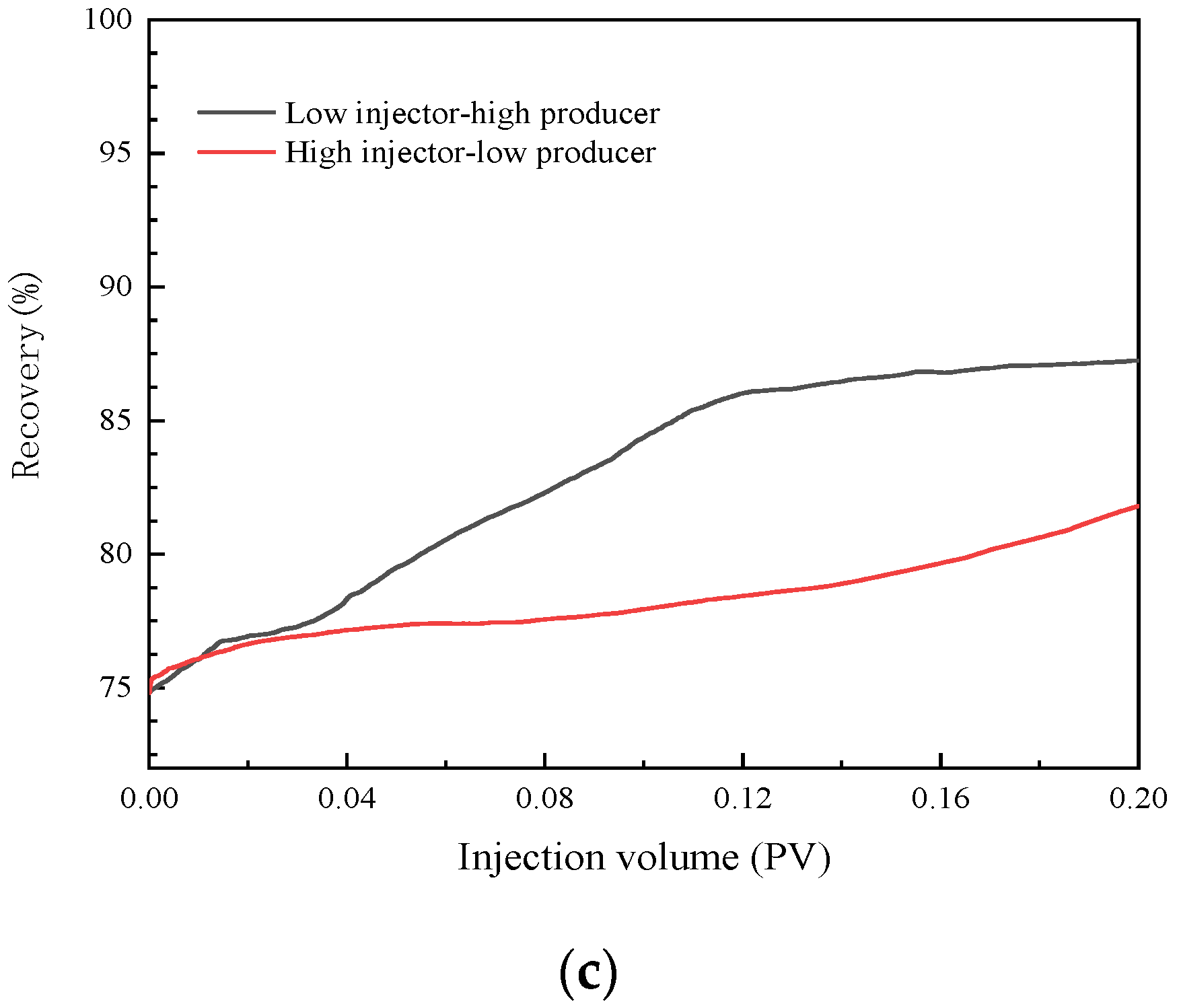
3.4.3. Effect of Injection–Production Relationship

Low injector–high producer and high injector–low producer modes were compared. The locations of injection and production wells and the distribution of reservoir fluid during nitrogen flooding are shown in Figure 9c and Figure 13. In the case of low injector–high producer mode, the attic oil between injection and production wells was effectively displaced. At the end of gas injection, the remaining oil formed at the bottom of the gas injection well (between gas cap and bottom water), and the middle area of the fracture–cavity structure. Under high injector–low producer mode, after the injection of gas from high point, a part of the original attic oil migrated to the lower location production well [7]. Part of the remaining oil flowed to other lower parts of the reservoir under the displacement of gas, forming a new distribution of trapped oil.

The water cut fluctuated greatly in low injector–high producer mode (<0.02 PV), and the injection gas and bottom water jointly displaced part of the remaining oil near the production well. With the increase of gas injection (>0.14 PV), part of the “attic oil” was also displaced to the production well at low point, and the corresponding water cut curve showed a decreasing trend. The water cut was lower compared with that of high injector–low producer mode (Figure 14a). Under the same conditions, gas channeling occurred when injection volume was 0.04 PV in low injector–high producer mode and 0.18 PV in high injector–low producer mode. During high injector–low producer mode, the injected gas migrates downwards from the high part of the structure, and its swept range was far bigger than that of low injector–high producer mode. Accordingly, gas channeling occurred in the production well at the low position after injecting a large volume of nitrogen (Figure 14b).

The additional recovery of low injector–high producer mode was 13.01%, which was much higher than that of high injector–low producer mode (8.06%), respectively. For high injector–low producer mode, although the injected gas had a wider sweep range, the remaining oil had not been produced due to the well pattern of one injector–one producer but migrated to other parts of the fracture–cavity structure (the right part of Figure 13c).

4. Conclusions

In this work, a reservoir-scale numerical conceptual model for simulating fractured-vuggy carbonate formation was established using CFD, based on the geological characteristics of a reservoir in Tahe oilfield, and was used to simulate the EOR process of nitrogen injection after water flooding. According to the simulation results, the mechanism of nitrogen flooding in this kind of reservoir includes displacing (replace) the remaining oil in high parts between injection and production wells (the remaining oil is visually defined as “attic oil”). In addition, the injection of nitrogen can help to change the swept range of bottom water. By changing the flow rate or gas injection mode of nitrogen injection, the swept area can be changed or disturbed in the flow process. The increased swept volume contributes to achieving a higher oil recovery. Nitrogen flooding can yield additional oil recovery of about 7–15% after water flooding, which proves that nitrogen flooding is an effective process to further enhance oil recovery in fractured-vuggy reservoirs after water flooding. Low-speed gas injection yields a higher oil recovery, but it may lead to a longer operation time and higher cost. High-speed gas injection can expand the swept area, but leads to faster gas channeling after gas breakthrough, accompanied by invalid swept volume and low oil recovery increment. Gas–water mixed injection can produce disturbance in reservoir and delay gas channeling. Under the same conditions, high injector–low producer mode can delay gas channeling, but the recovery increment is greatly affected by the well pattern.

The numerical simulation method used in this work helped the understanding of the fluid migration and distribution characteristics under different displacement modes in fracture-vuggy reservoirs, which cannot be effectively simulated at present by traditional reservoir simulation methods, based on seepage theory. Additionally, the simulation method, using CFD, makes up for the deficiency of physical simulation experiments, and helps to clarify the influence of various factors on nitrogen flooding EOR process and provide a more in-depth understanding regarding the mechanism of nitrogen flooding in fractured-vuggy reservoirs. It was found that there is a synergistic effect between injected gas and bottom water, and an imperfect injection production well pattern may result in a low oil recovery by high injector–low producer mode, which still needs further study. Numerical simulation shows that there is still a lot of residual oil in fractured-vuggy reservoir after nitrogen flooding in the trapped area, formed by a gas cap and bottom water. The question of how to further enhance oil recovery after gas flooding is one worthy of more attention.

References

1. Jiao, F. Practice and knowledge of volumetric development of deep fractured-vuggy carbonate reservoirs in Tarim Basin, NW China. Shiyou Kantan Yu Kaifa/Pet. Explor. Dev. 2019, 46, 552–558. [Google Scholar] [CrossRef]
2. Hu, W. Development technology and research direction of fractured- vuggy carbonate reservoirs in Tahe OilfieldDevelopment technology and research direction of fractured- vuggy carbonate reservoirs in Tahe Oilfield. Reserv. Eval. Dev. 2020, 10, 1–10. [Google Scholar]
3. Wei, Z.; Gang, H.A.I.; Ying, Z. Gas-Water Composite Flooding Technology for Fractured and Vuggy Carbonate Reservoirs in Tahe Oilfield. Pet. Drill. Tech. 2020, 48, 61–65. [Google Scholar] [CrossRef]
4. Tan, T.; Guo, C.; Chen, Y.; Dou, L.; Company, O. Study and practice on mechanism of EOR by N2 flooding in fractured-vuggy reservoirs with high temperature and high pressure. Reserv. Eval. Dev. 2020, 10, 60–64. [Google Scholar]
5. Lyu, X.; Liu, Z.; Hou, J.; Lyu, T. Mechanism and influencing factors of EOR by N2 injection in fractured-vuggy carbonate reservoirs. J. Nat. Gas Sci. Eng. 2017, 40, 226–235. [Google Scholar] [CrossRef]
6. Hou, J.; Zhang, L.; Li, H.; Li, W.; Yuan, D.; Yuan, Y.; Zheng, Z. Influencing factors on EOR nitrogen flooding in fractured-vuggy carbonate reservoir. Pet. Geol. Recover. Effic. 2015, 22, 64–68. [Google Scholar]
7. Xiaojun, C. Visualized Gas Drive EOR Experiments in Fractured-Vuggy Reservoirs after Waterflooding in Tahe Oilfield. Xinjiang Pet. Geol. 2018, 39, 473–479. [Google Scholar]
8. Zheng, Z.; Zhu, T.; Hou, J.; Luo, M.; Gao, Y. Visible research on remaining oil after nitrogen flooding in fractured-cavity carbonate reservoir. Pet. Geol. Recover. Effic. 2016, 23, 93–97. [Google Scholar]
9. Qu, M.; Hou, J.; Zhao, F.; Song, Z.; Ma, S.; Wang, Q.; Li, M.; Yang, M. 3-D visual experiments on fluid flow behavior of water flooding and gas flooding in fractured-vuggy carbonate reservoir. In Proceedings of the SPE Annual Technical Conference and Exhibition, San Antonio, TX, USA, 9–11 October 2017; p. SPE187273. [Google Scholar]
10. Yang, J.; Hou, J. Experimental study on gas channeling characteristics of nitrogen and foam flooding in 2-D visualized fractured-vuggy model. J. Pet. Sci. Eng. 2020, 192, 107337. [Google Scholar] [CrossRef]
11. Yang, J.; Hou, J.; Qu, M.; Liang, T.; Wen, Y. Experimental study the flow behaviors and mechanisms of nitrogen and foam assisted nitrogen gas flooding in 2-D visualized fractured-vuggy model. J. Pet. Sci. Eng. 2020, 194, 107501. [Google Scholar] [CrossRef]
12. Wang, J.; Ji, Z.; Liu, H.; Huang, Y.; Wang, Y.; Pu, Y. Experiments on nitrogen assisted gravity drainage in fractured-vuggy reservoirs. Pet. Explor. Dev. 2019, 46, 355–366. [Google Scholar] [CrossRef]
13. Qu, M.; Hou, J.; Wen, Y.; Liang, T. Nitrogen gas channeling characteristics in fracture-vuggy carbonate reservoirs. J. Pet. Sci. Eng. 2020, 186, 106723. [Google Scholar] [CrossRef]
14. He, J.; Killough, J.E.; Gao, S.; Fadlelmula, M.M.; Michael Fraim, F. Confronting the simulation of fluid flow in naturally fractured carbonate karst reservoirs. In Proceedings of the Society of Petroleum Engineers—Abu Dhabi International Petroleum Exhibition and Conference 2016, Abu Dhabi, United Arab Emirates, 7–10 November 2016; p. SPE183143. [Google Scholar]
15. Zhang, H.; Lv, X.; Liu, Z.; Han, K. A Study on Fracture Vuggy Reservoir Multi-scale Flow Simulation Based on Pseudo-particle Method. J. Southwest Pet. Univ. Technol. Ed. 2014, 36, 93–100. [Google Scholar]
16. Wu, Y.S.; Di, Y.; Kang, Z.; Fakcharoenphol, P. A multiple-continuum model for simulating single-phase and multiphase flow in naturally fractured vuggy reservoirs. J. Pet. Sci. Eng. 2011, 78, 13–22. [Google Scholar] [CrossRef]
17. Gao, Y.; Li, X.; Peng, X. Study on Equivalent Simulation Method of Large-scale Fracture Cavity Body in Fracture Cavity Reservoir. J. Yangtze Univ. Sci. Ed. 2016, 13, 66–69. [Google Scholar]
18. Yong, L.; Baozhu, L.; Qi, W.; Xingliang, D. Different equivalent simulation methods for fractured-vuggy carbonate gas condensate reservoirs. In Proceedings of the Society of Petroleum Engineers—SPE Europec featured at 79th EAGE Conference and Exhibition, Paris, France, 12–15 June 2017; pp. 1393–1404. [Google Scholar] [CrossRef]
19. Yan, X.; Huang, Z.; Yao, J.; Zhang, Z.; Liu, P.; Li, Y.; Fan, D. Numerical simulation of hydro-mechanical coupling in fractured vuggy porous media using the equivalent continuum model and embedded discrete fracture model. Adv. Water Resour. 2019, 126, 137–154. [Google Scholar] [CrossRef]
20. Kang, Z.; Li, Y.; Ji, B. Key technologies for EOR in fracture-vuggy carbonate reservoirs. OIL GAS Geol. 2020, 41, 434–441. [Google Scholar]
21. Kang, Z.; Wu, Y.S.; Li, J.; Wu, Y.; Zhang, J.; Wang, G. Modeling multiphase flow in naturally fractured vuggy petroleum reservoirs. In Proceedings of the SPE Annual Technical Conference and Exhibition, San Antonio, TX, USA, 24–27 September 2006; Volume 3, pp. 1794–1803. [Google Scholar] [CrossRef]
22. Wu, Y.S.; Qin, G.; Ewing, R.E.; Efendiev, Y.; Kang, Z.; Ren, Y. A multiple-continuum approach for modeling multiphase flow in naturally fractured vuggy petroleum reservoirs. In Proceedings of the International Oil & Gas Conference and Exhibition in China, Beijing, China, 5–7 December 2006; Volume 2, pp. 739–750. [Google Scholar] [CrossRef]
23. Kiran, R.; Ahmed, R.; Salehi, S. Experiments and CFD modelling for two phase flow in a vertical annulus. Chem. Eng. Res. Des. 2020, 153, 201–211. [Google Scholar] [CrossRef]
24. Fu, H.; Yang, L.; Liang, H.; Wang, S.; Ling, K. Diagnosis of the single leakage in the fluid pipeline through experimental study and CFD simulation. J. Pet. Sci. Eng. 2020, 193, 107437. [Google Scholar] [CrossRef]
25. Ge, Z.; He, D.; Huang, R.; Zuo, J.; Luo, X. Application of CFD-PBM coupling model for analysis of gas-liquid distribution characteristics in centrifugal pump. J. Pet. Sci. Eng. 2020, 194, 107518. [Google Scholar] [CrossRef]
26. Yan, T.; Qu, J.; Sun, X.; Chen, Y.; Hu, Q.; Li, W.; Zhang, H. Numerical investigation on horizontal wellbore hole cleaning with a four-lobed drill pipe using CFD-DEM method. Powder Technol. 2020, 375, 249–261. [Google Scholar] [CrossRef]
27. Zhang, R.; Bo, K.; Liu, Z. A method of sizing plugging nanoparticles to prevent water invasion for shale wellbore stability based on CFD-DEM simulation. J. Pet. Sci. Eng. 2021, 196, 107733. [Google Scholar] [CrossRef]
28. Azadi, M.; Aminossadati, S.M.; Chen, Z. Large-scale study of the effect of wellbore geometry on integrated reservoir-wellbore flow. J. Nat. Gas Sci. Eng. 2016, 35, 320–330. [Google Scholar] [CrossRef] [Green Version]
29. Sami, N.A.; Turzo, Z. Computational fluid dynamic (CFD) simulation of pilot operated intermittent gas lift valve. Pet. Res. 2020, 5, 254–264. [Google Scholar] [CrossRef]
30. Sami, N.A.; Turzo, Z. Computational fluid dynamic (CFD) modelling of transient flow in the intermittent gas lift. Pet. Res. 2020, 5, 144–153. [Google Scholar] [CrossRef]
31. Liu, C.; Li, J.; Song, Y. Study on the flow of water drive in cavern of fractured-cave reservoirs. Hebei J. Ind. Sci. Technol. 2018, 35, 171–177. [Google Scholar]
32. Pinilla, A.; Asuaje, M.; Hurtado, C.; Hoyos, A.; Ramirez, L.; Padrón, A.; Ratkovich, N. 3D CFD simulation of a horizontal well at pore scale for heavy oil fields. J. Pet. Sci. Eng. 2021, 196, 107632. [Google Scholar] [CrossRef]
33. Mehraban, M.F.; Rostami, P.; Afzali, S.; Ahmadi, Z.; Sharifi, M.; Ayatollahi, S. Brine composition effect on the oil recovery in carbonate oil reservoirs: A comprehensive experimental and CFD simulation study. J. Pet. Sci. Eng. 2020, 191, 107149. [Google Scholar] [CrossRef]
34. Liu, C.; Liu, G.; Li, J.; Yan, Z. Anaylysis of mechanism and influential factors of water-driven-oil in fractured-vuggy reservoirs based on Fluent and Hernandez. J. Nanjing Univ. Sci. Technol. 2019, 43, 367–372. [Google Scholar]
35. Mudunuru, M.K.; Carey, J.W.; Chen, L.; Kang, Q.; Karra, S.; Vesselinov, V.V.; Middleton, R.S.; Johnson, P.A.; Viswanathan, H.S. Subsurface energy: Flow and reactive-transport in porous and fractured media. In Handbook of Porous Materials: Synthesis, Properties, Modeling and Key Applications; World Scientific: Singapore, 2020; Volume 4, pp. 323–395. [Google Scholar] [CrossRef]
36. Mudunuru, M.K.; O’Malley, D.; Srinivasan, S.; Hyman, J.D.; Sweeney, M.R.; Frash, L.; Carey, B.; Gross, M.R.; Welch, N.J.; Karra, S.; et al. Physics-informed machine learning for real-time unconventional reservoir management. CEUR Workshop Proc. (No. LA-UR-19-31611); Los Alamos National Lab. (LANL): Los Alamos, NM, USA, 2020; Volume 2587. [Google Scholar]
37. Gross, M.R.; Hyman, J.D.; Srinivasan, S.; O’Malley, D.; Karra, S.; Mudunuru, M.K.; Sweeney, M.; Frash, L.; Carey, B.; Guthrie, G.D.; et al. A Physics-informed Machine Learning Workflow to Forecast Production in a Fractured Marcellus Shale Reservoir. In Proceedings of the SPE/AAPG/SEG Unconventional Resources Technology Conference, Houston, TX, USA, 26–28 July 2021; pp. 1–8. [Google Scholar] [CrossRef]
Figure 1. Seismic profile of TK411 well group.
Energies 14 07554 g001
Figure 2. Surface weathering—underground river karst model.
Energies 14 07554 g002
Figure 3. Conceptual numerical model.
Energies 14 07554 g003
Figure 4. Original oil–water distribution (red—oil; light blue—water).
Energies 14 07554 g004
Figure 5. Fluid distribution in different displacement stages of 60 MPa bottom water: (a) initial stage; (b) last stage.
Energies 14 07554 g005
Figure 6. Production curves of bottom water flooding stage.
Energies 14 07554 g006
Figure 7. Fluid distribution in different displacement stages of water injection: (a) initial stage; (b) last stage.
Energies 14 07554 g007
Figure 8. Production curves of artificial water injection stage.
Energies 14 07554 g008
Figure 9. Fluid distribution in nitrogen injection with different flow rates: (a) initial time of gas flooding; (b) 20,000 m3/d; (c) 50,000 m3/d; (d) 80,000 m3/d.
Energies 14 07554 g009aEnergies 14 07554 g009b
Figure 10. Production curves under different flow rate: (a) water cut; (b) gas production rate; (c) cumulative recovery.
Energies 14 07554 g010
Figure 11. Fluid distribution in different nitrogen injection modes: (a) initial time at nitrogen injection; (b) intermittent mode; (c) gas–water mixed mode; (d) gas–water alternate mode.
Energies 14 07554 g011
Figure 12. Production curves under different injection modes: (a) water cut; (b) gas production rate; (c) cumulative recovery.
Energies 14 07554 g012
Figure 13. Fluid distribution in different stages of high injector–low producer mode: (a) initial stage; (b) last stage.
Energies 14 07554 g013
Figure 14. Production curves under different relationship: (a) water cut; (b) gas production rate; (c) cumulative recovery.
Energies 14 07554 g014aEnergies 14 07554 g014b