Abstract
In this paper, testing and diagnosis methods for the static excitation systems of power plant synchronous generators using Hardware-In-the-Loop technology are described. These methods allow a physical excitation system to be connected to a real-time model of a power plant unit. A feature of a static excitation system is the presence of generator self-excitation—that is, when the input voltages of the excitation system are defined by a synchronous generator. These voltages are determining by the digital model, which creates additional difficulties with combining a digital model with a real excitation system. Various ways to solve this problem are described in this article; in particular, we focus on the option in which the gate-impulses of a thyristor converter are applied to the digital model by a real static excitation system. The real-time models are based on the method of average voltages in the integration step. This method is effective for providing numerical stability for the models of power schemes and their functioning in real time mode over a long period. A synchronization method for the calculation time of the model with real time is described. The adequacy of the described method is proved by the results of the static excitation system of synchronous generators testing in operating and fault modes.
1. Introduction
Based on Hardware-In-the-Loop (HIL) technology, hybrid models combine physical objects and real-time models [1]. This technology is widely used for testing control devices, in particular when using Model-Based Design (MBD) methods [2,3]. Connecting control devices to the control object in the form of a real-time model provides control system synthesis, testing, and fault diagnosis. Nowadays, these methods are widely used in the automotive [4,5] and aerospace [6,7] industries. For example, in [4] the authors propose to use a HIL platform for testing different control strategies for the adaptive cruise control of vehicles. Based on HIL technology, [6] proposed a testing process in which a flight control system (autopilot) is connected to a digital model of the target aircraft. As noted in [8], the HIL simulation technique is an effective approach for performing cost-effective system-level testing. Additionally, in [8] it is proposed to use the HIL simulation technique for testing special protection systems in large-scale power systems.
Combining the physical objects and real-time models of the absent components in a single unit expands the possibilities of complex-systems analysis and can be used for research and training [9]. HIL-based optimization methods are used for the synthesis of control systems [10].
The use of Hardware-In-the-Loop technology for electrical power engineering allows one to solve a set of problems connected to the synthesis of energetics–objects control systems. The use of a real-time simulator of a power grid with a wind power plant for an operation-mode analysis and control-system synthesis is described in [11]. A real-time simulator of a doubly fed induction machine that can be used for control-system synthesis and testing is presented in [12]. A real-time model of a DTC electric drive for a locomotion module is described in [13] and proposed for use in hybrid systems, combining the computer models of the AC e-motor and the physical e-motors of several locomotion modules.
An important task for electrical power engineering is to synthesize and diagnose the excitation systems of power-unit generators. This task can be solved effectively by using real-time simulation and Hardware-In-the-Loop technology [14,15,16]. Both special real-time systems and personal computers with Windows operating systems are used simultaneously for an implementation of the real-time models [11].
Static excitation systems are widely used for the field regulation of low and medium synchronous generators, in which the field current is regulated by a controlled rectifier—for example, by a thyristor converter (Figure 1) [17,18,19]. Instead of using a thyristor converter, a pulse-width converter can be used for low-power generators [20]. The advantage of such a system is the high rapidity of the excitation control, which favorably distinguishes them from electromachine (brushless) excitation systems [21]. The self-excitation of synchronous generators is used in most of these systems. This creates a difficulty by combining a physical excitation system with a real-time model of the power unit.
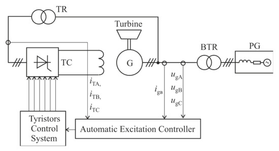
Figure 1.
Static excitation system of synchronous generators: G—synchronous generators; BTR—generator’s transformer; PG—power grid; TR—input transformer of excitation system; TC—thyristor converter.
A proposal in [22] is to use a power system real-time model integrated into the automatic excitation controller for testing the power system stabilizer of a generator with static excitation systems. Such integration allows the self-diagnosis of the control system; however, the limited computing performance of the controller compared to the PC does not allow a sufficiently complete description of the power generation system to be given. An RTDS simulation tool was used to create a real-time model in [22].
Another problem is choosing a method for the development of a real-time model that would provide calculation performance and numerical stability over a long period of continuous model functioning. This issue has been noted previously, specifically in [11,12,22].
The purpose of this article is to present a concept for diagnosing the static excitation systems of synchronous generators using Hardware-In-the-Loop technology, to describe the mathematical and digital real-time models created using the method of the average voltages in the integration step (AVIS), and to provide an example of an application that confirms the adequacy of the models developed and solutions proposed.
2. Diagnosis Technology
The testing and diagnosis tasks of the excitation systems of synchronous generators are to check the excitation system in the operating modes, the correctness of the protection system’s functioning in fault modes, the compliance of the regulation characteristics, and the adjustment of the automatic protection-and-control-system configuration, as well as to search for possible faults when a defect is detected. Such diagnosis must be performed after the excitation system is produced and before its commissioning, as well as periodically at the power plant during planned preventive shutdowns of the power unit.
In order to diagnose the excitation system, it is connected to the digital real-time model of the power scheme of the power-generation system (Figure 2). This model includes a synchronous generator (G), the generator’s transformer (BTR), a power grid (PG), the input transformer of the excitation system (TR) (the excitation-system transformer), and a thyristor converter (TC).
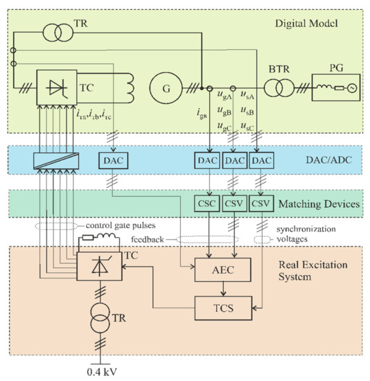
Figure 2.
Functional scheme for diagnosing the excitation system.
This digital model must replace an absent object (power unit) during the testing of the excitation system. The signals of the stator-phase voltages (instantaneous values ugA, ugB, and ugC), input currents of the thyristor converter (instantaneous values iTA, iTB, and iTC) or field current, and stator phase current (instantaneous value of stator current for B phase igB) are sent from the real-time model to the excitation system, and are needed in order for the excitation system to function. A specific list of the required signals is determined by the excitation system, which is diagnosed. Digital-to-analog converters (DAC) and matching devices (amplifiers) are used to form these signals. Matching devices must provide the required level and power of the signals and the galvanic separation.
A feature of a static excitation system is the presence of generator self-excitation. In this case, the input voltages of the excitation system (the excitation-system thyristor converter (TC)) are the output voltages of the excitation-system transformer (TR), which is connected to the synchronous generator terminals (Figure 1). These voltages are determined by the digital model, which creates additional difficulties for combining a digital model with a real excitation system. These are the options for overcoming them:
- Option 1. A very expensive power amplifier can be used to supply the real excitation system with the calculated voltages of the excitation-system transformer (TR) from the digital model. The excitation voltage from the thyristor converter of the real excitation system is applied to the digital model. The thyristor converter is connected to the RL load, the parameters of which correspond to the field-winding parameters of the synchronous generator. Such an option tests the entire power circuit of the excitation system but significantly increases the diagnosis cost due to the need for a power amplifier with high dynamic characteristics and significant gain.
- Option 2. This option is shown in Figure 2. The calculated voltages of the excitation-system transformer (TR) in the digital model are applied to the gate pulse control system (TCS) of the thyristor converter in the real excitation system (as the synchronization voltages forming the gate pulses). In this case, the power of the amplifier is much smaller because the gate pulse control system does not consume a significant amount of power. The control gate pulses are applied to the digital model from a real excitation system. In this case, the circuits of the gate pulse control system (TCS) and the automatic excitation controller (AEC) are tested.
- Option 3. The output signal of the automatic excitation controller (AEC) is applied to the digital model from the real excitation system (the control signal for the thyristor converter). The calculated feedback signals needed for the automatic excitation controller to function are applied to the real excitation system from the digital model. Thus, only the automatic excitation controller is tested, not the control circuits or power scheme of the thyristor converter.
In our opinion, Option 2 is optimal. It allows the testing of the excitation controller, as well as the control circuits of the thyristor converter, but not its power scheme. At the same time, Option 2 does not require an expensive amplifier to supply the excitation system with a voltage calculated in a digital model. The power scheme of the thyristor converter can be tested separately, and the presence of a generator unit (or its digital model) is not required for such testing.
An image of the diagnosis complex developed for this study is shown in Figure 3.
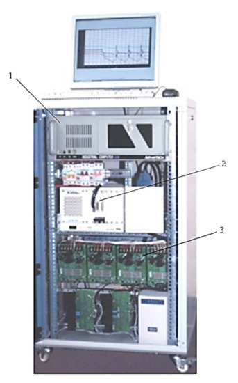
Figure 3.
Image of the diagnosis complex used: 1—industrial computer; 2—DAC/ADC cards; 3—matching devices.
The multifunction I/O modules with analog-to-digital converters and digital-to-analog converters (type NI PXI–6259 National Instruments) were used for the information transfer between the digital model and peripheral analog devices. These modules included 32 analog inputs (16-bit, 1.25 MS/s), 4 analog outputs (16-bit, 2.8 MS/s), and 48 digital inputs/outputs. For the second option, six digital inputs were used for transferring the control gate impulse from the excitation system thyristor converter to the digital model. I/O modules were placed on a PXI-1033 chassis, which is designed for distributed data collection and processing (item 2 in Figure 3).
Transforming the DAC signal by power and level provided amplifiers (item 3 in Figure 3). These amplifiers were set to be current or voltage sources and were regulated by ±10 V signals from the DAC output.
3. Mathematical Model Description
A mathematical model used for the diagnosis of an excitation system must meet the following requirements: the non-linearity of the electric machines and thyristor converters must be taken into consideration for the model to be adequate in the operating and fault modes; the model must provide a high calculation performance and high accuracy when increasing the integration step; finally, it must provide numerical stability for the calculation over a long period of continuous functioning.
One feature of the proposed approach is that it uses a method of average voltages in the integration step (AVIS) for the algebraization of the differential equations that describe the power scheme. The theoretical foundations of this method were first described by the author in [23]. The main specifications of this method and its development for modeling a nonlinear power scheme are described in [15,16]. The advantages of this AVIS method over other methods are noted in [11]. Numerical stability in this method is provided by solving equations for the power scheme in which the algebraic sum of the voltages is zero at the beginning of the integration step and in which the algebraic sum of the currents is zero at the end of the integration step. According to the classic methods, there are no explicit equations for the currents to sum to zero (the explicit methods) or for the voltages to sum to zero (implicit methods).
According to this AVIS method, the equation for an electric branch which includes an electromotive force source e and inductance and resistance R with applied voltage u on its terminals is written as:
where and are the average values of the applied voltage and electromotive force in the step, (i1 − i0) is the branch current increment in the integration step, (ψ1 − ψ0) is the increment of the flux linkages in the integration step, m is the order of polynomial that describes the branch current in the integration step and determines method order, and ∆t is the integration step value.
Mathematical models of the power scheme elements (the synchronous machine, transformer, power grid, and thyristor converter) are based on Equation (1). The calculation schemes of these elements are represented as multipoles.
As an example, let us consider the model of a synchronous machine using the first-order AVIS method (m = 1). It is represented by an eight-pole, the poles of which are the ends of the stator winding and the excitation winding. After applying Equation (1) to this scheme, we obtain the following vector equation that connects the potentials of the poles and and the currents of the external branches . Thus:
where is the matrix of the resistances of the stator winding and excitation winding. The indices 1 and 0 refer to the values of the variables at the beginning and end of the integration step, respectively.
The damping system of the synchronous machine is modeled by two short-circuited branches oriented on axes (d, q) and includes resistances rD and rQ together with inductances. It is described by the following internal vector equation for the currents of the internal branches :
where is the matrix of the resistances of the damping winding.
In Equations (2) and (3), and are the vectors of the flux linkages of the external and internal circuit. Their changes in the integration step are defined as follows:
where and are the matrices of the self and mutual inductances of the external and internal circuit and are the matrices of the mutual inductances between the external and internal circuits.
Equations (2) and (3), using Equations (4) and (5), are written as:
where , , and are the matrices of the step resistances of the external and internal circuits.
The mathematical model of the electrical part of the synchronous machine, represented as a multipole, is presented by the following equation:
where is the vector of the external poles’ potentials; is the vector of the current in the external branches; ; is the matrix of coefficients; and is the vector of the absolute values, in which the vector of e.m.f is defined as:
The mechanical part of the synchronous machine is described by the following equation:
where TS is the electromagnetic torque of the synchronous machine, ω is the rotor rotation speed, J is the moment of inertia, and Tt is the turbine torque. The latter is determined by taking into consideration the active power and speed controller as well as the inertia of the turbine according to the following equation:
where kP and kω are the gain of the power and speed controller, respectively, and Pt and ωt are the reference values of the turbine power and speed, respectively.
The mathematical model of the synchronous machine using the second-order AVIS method is described in [15]. Its advantage is its higher accuracy of calculation at the same step of numerical integration. However, it requires one to determine the derivative currents and perform more calculations in the step.
Mathematical models of the other elements-multipoles (transformer, power grid, thyristor converter) are presented in the form of Equation (8). They are combined into a single system using equations compiled according to Kirchhoff’s first law for the system’s nodes, in which the elements’ outer branches are connected. The method for connecting the elements is described using incidence matrices. The calculation algorithm is described in [15].
Another feature of the proposed approach is that it takes into consideration the discretization of the controlled rectifier thyristors in the mathematical model. It allows the prediction of the system’s behavior in the case of thyristor fault. The power scheme of the thyristor converter (a three-phase, full-bridge rectifier) is represented as a scheme with a constant structure and variable parameters. The semiconductor switches (thyristors) are represented as having serial connected resistances and inductances with low values in the “on” state and high values in the “off” state. The switch turns on when an pulse from the gate control system of the real thyristor converter is present. The switch instantly turns off when its current crosses zero, passing from a positive to a negative value. The mathematical model of such a semiconductor converter is described in [13].
The authors’ object-oriented method and program environment, realized on C++, was used for the computer application of the models developed. The program environment allowed us to create the models with a graphical user interface for realizing the operating and fault modes of the power-unit. In addition, it was possible to register and visualize the testing results.
4. Time Synchronization
A feature of the real-time model that works with real objects is the need to synchronize the calculated time of the model (it is integrated with the other variables) in real time. The difference between the calculated time and real time leads to the system exhibiting inadequate dynamic behavior. In addition, in this case there is a difference between the calculated generator frequency and its reference value, as determined by the turbine speed.
Synchronizing the calculated time of the model with the real time is required when digital models are implemented using equipment in which the performance and calculated time can vary (for example, the implementation of a digital model on a PC with a Windows system). The use of a special real-time system partly solves this problem but creates other difficulties.
The real time must be measured in order to synchronize it with the calculated time of the model. The internal PC timer can be used for this purpose using the QueryPerformanceCounter C-function. The error caused by time measuring discretization must be eliminated in order to determine the real time at any moment. To do this, the timer reading tTIME was approximated using the least-squares method. Approximating the dependence was determined according to the equation tTIME = atREAL, where a must equal 1 (the dotted line in Figure 4).
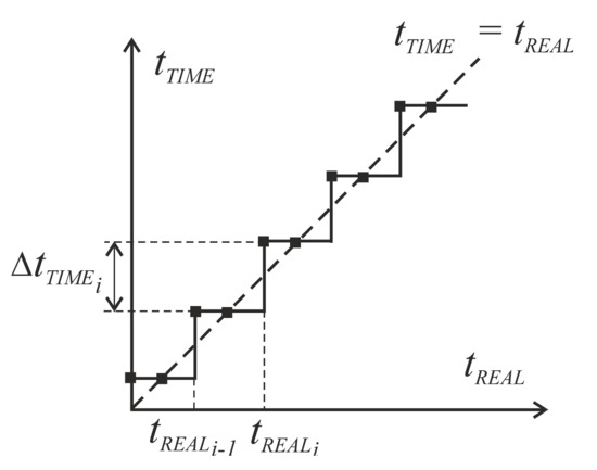
Figure 4.
Approximation of timer reading values for time synchronization.
Given that a necessary condition of the model functioning in real-time mode is to equalize the calculated time and real time (tREAL = tCALC), the ratio of the calculated time of the model to the real time (measured by the timer) was determined using the equation
tTIME = atCALC.
According to the least-squares method, the ratio a is written as:
where N is the quantity of measurement, tTIME.i is the timer reading in the i-th integration step, and tCALC.i is the calculated time in the i-th integration step. Note that the timer was read at each integration step.
According to Equation (11), the ratio a equals 1 when the model functions in real-time mode. In other cases, if the calculation speed is changing and there is a difference between the calculated time of the model and the real time, then the ratio a does not equal 1. This means that a correction of the calculation speed (the calculated time in the model) is needed. The calculation speed or response can be changed by changing the integration step.
The integration step on each calculated cycle was determined on the basis of the previous value, which is averaged for N previous cycles according to following equation:
Such an approach provides the automatic correction of the integration step when the model is in real-time mode. If the calculated step according to Equation (12) exceeds the maximum allowable value, this means that the mathematical model cannot function in real-time mode on this computer. In this case, a computer with a higher performance must be used.
Another method of time synchronization is to determine the numerical integration step value based on the measurement of the instantaneous voltages in the three-phase AC network. It is known that the voltage frequency of the network is quite stable (in the normal operation of the continental European power system, it is considered to be within 50 Hz ± 50 mHz [24]). This allows using the network voltage to determine the time quite accurately.
In this case, the increment of the voltage vector’s angular position during one calculation cycle (numerical integration step) is defined as:
where and are the voltages in the (α,β) coordinate frame and is the amplitude of the voltage.
In order to equalize the calculated time and real time (tREAL = tCALC), the integration step is calculated as:
where f is the frequency of the voltage, which is equal to 50 Hz.
5. Results
The adequacy of the approach proposed and hybrid models developed was verified by comparing the results (using an oscillogram) obtained from the hybrid system created—in which the real excitation system operates with a digital model of the generator unit—with experimental results obtained from a real power generation system at Burshtyn Thermal Power Plant (Ukraine). The parameters of the power scheme are as follows.
For the synchronous generator: the nominal power (Sn) was 235 MVA, the nominal voltage (Un) was 15 kV, the nominal current (In) was 7300 A, the field current in a no-load regime (if) was 720 A, the stator-winding resistance was 0.00148 Ohm, and the resistance of the field winding (rf) was 0.223 Ohm. The reactances were: Xd = 1.84 p.u., Xad = 1.68 p.u., Xq = 1.84 p.u., Xaq = 1.68 p.u., X’d = 0.295 p.u., X’’d = 0.19 p.u., and X’’q = 0.19 p.u. The number of pole pairs p0 = 1. The moment of inertia (J) was 6000 kgm2.
For the power transformer BTR: the nominal power (Sn) was 250,000 kVA, the voltage of the primary winding (U1n) was 15 kV, the nominal voltage of the secondary winding (U2n) was 347 kV, the no-load current (I0) was 0.062 p.u., the short-circuit voltage (Usc) was 0.11 p.u., and the active power loss was 955 kW.
For the excitation system transformer TR: the nominal power (Sn) was 2500 kVA, the nominal voltage of the primary winding (U1n) was 15 kV, the nominal voltage of the secondary winding (U2n) was 863 V, the no-load current (I0) was 0.09 p.u., the short-circuit voltage (Usc) was 0.065 p.u., and the active power loss was 22 kW.
A comparison of the results obtained in the created hybrid system and the experimental results is shown in Figure 5 for the initial excitation operating mode, in Figure 6 for the de-excitation operating mode, and in Figure 7 for the short circuit in power line. The results of this comparison confirm the adequacy of the models developed and approach proposed.
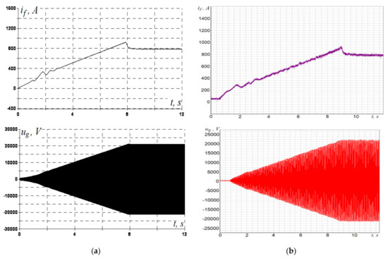
Figure 5.
(a) Simulation in the hybrid system; (b) experimental results of the field current (if) and terminal voltage of the generator (ug, instantaneous value) for the initial excitation of the generator.
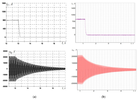
Figure 6.
(a) Simulation in the hybrid system; (b) experimental results of the field current (if) and terminal voltage of the generator (ug, instantaneous value) for the de-excitation of the generator.
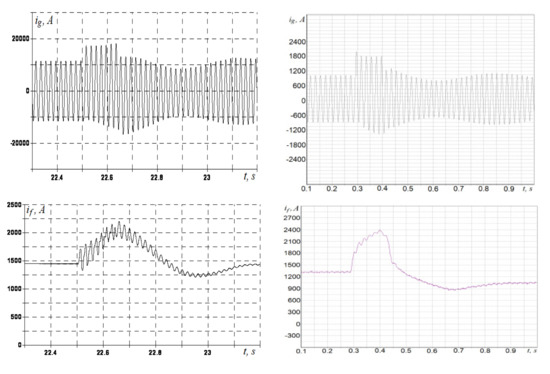
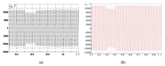
Figure 7.
(a) Simulation in the hybrid system; (b) experimental results of the stator current (ig), field current (if), and phase voltage of the generator (ug) for the one-phase short circuit on the power line.
The oscillogram for the connection of the generator to the power grid and the active power loading through a sharp change in turbine power are shown in Figure 8 and Figure 9, respectively. Such a type of power change was chosen in order to evaluate the operation of the excitation controller in the most difficult operating mode in comparison with a smooth power increase. The generator was connected to the power grid at 13 s, when the condition of exact synchronization had been reached. Therefore, this mode was not accompanied by significant current pulsation (Figure 8a)
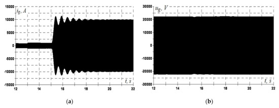
Figure 8.
(a) Stator current (ig, instantaneous value); (b) terminal voltage of the generator (ug, instantaneous value) for connecting the generator to the power grid (at 13 s) and the active power loading (at 15 s).
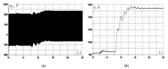
Figure 9.
(a) Field voltage (uf); (b) field current (if) for connecting the generator to the power grid (at 13 s) and the active power loading (at 15 s).
The sharply changing active power loading occurred at 15 s and was achieved by increasing the active power supplied to the generator by the turbine. In this case, there was current pulsation as the current increased to a nominal value (Figure 8a). Th excitation controller with the PI voltage controller in the diagnosed excitation system provided insignificant dynamic error (1.8%) when the active power changed sharply. The static error of voltage regulation is absent (Figure 8b).
The oscillogram of the frequency decrease when the synchronous generator was not loaded is shown in Figure 10. The frequency decrease was achieved by reducing the turbine speed. The excitation controller provided the stabilization of the magnetic flux for the prevention of the magnetic circuit saturation. The protection system disabled the generator excitation when the frequency was reduced to a critical value (about 45 Hz). There was a de-excitation of the synchronous generator. The field current was reduced to zero within 0.8 s due to the thyristor converter being switched to inverter mode. The time to terminal-voltage reduction (de-excitation time) was 4.0 s, as the magnetic flux was maintained by the damper system of the generator.
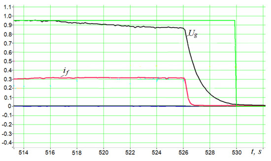
Figure 10.
The results of protection system operation during a frequency decrease in a no-loaded generator: Ug is the RMS value of the generator voltage, if is the field current.
A feature of the proposed approach is that testing the excitation system in case of thyristor fault is possible. A thyristor fault (i.e., when the thyristor does not turn on) can be physically realized by disconnecting the gate impulse from the digital model. Such results are shown in Figure 11. As the test results in this mode show, the excitation system retained its efficiency and restored the required value of the excitation current for 1.5 s. The field current exhibited pulsation in this case, but it did not influence the terminal voltage of the generator.
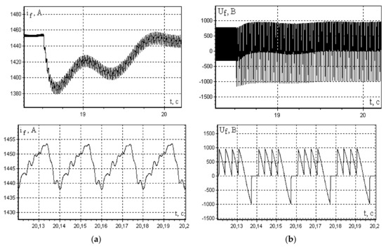
Figure 11.
(a) Field voltage (uf); (b) field current of the generator (if) in the case of a thyristor fault (i.e., when the thyristor does not turn on).
6. Conclusions
The proposed approach enables testing and diagnosing the excitation systems of synchronous generators using the real-time model of a power-unit scheme. A feature of this approach is that it takes into consideration the nonlinearity of the synchronous machine and the discretization of the thyristor’s functioning in a mathematical model. It allows fault situations to be realized: that is, short circuits in the generator terminals and thyristor faults of the controlled rectifier. The method of average voltages in the integration step was used in the developed model because of its high calculation speed, which enables the model to function in real time. In addition, this method provides numerical stability to the model over a long period (about 12 h of continuous functioning). This method is sufficient to test the excitation system in operating and fault modes.
Author Contributions
Conceptualization, A.K.; methodology, A.K. and M.S.; software, M.S.; validation, A.K., M.K. and G.P.; formal analysis, M.K.; investigation, A.K., M.S. and M.K.; resources, G.P.; data curation, M.S. and G.P.; writing—original draft preparation, A.K. and M.S.; writing—review and editing, A.K. and M.K.; visualization, M.S. All authors have read and agreed to the published version of the manuscript.
Funding
This research received no external funding.
Institutional Review Board Statement
Not applicable.
Informed Consent Statement
Not applicable.
Data Availability Statement
Data available on request to the author.
Conflicts of Interest
The authors declare no conflict of interest.
References
- Bélanger, J.; Venne, P.; Paquin, J.-N. The what, where, and why of real-time simulation. Planet RT 2010, 1, 37–49. [Google Scholar]
- Fang, K.; Zhou, Y.; Ma, P.; Yang, M. Credibility evaluation of hardware-in-the-loop simulation systems. In Proceedings of the 2018 Chinese Control and Decision Conference (CCDC), Shenyang, China, 9–11 June 2018; pp. 3794–3799. [Google Scholar] [CrossRef]
- Conner, K. An Introduction to Hardware-in-the-loop (HIL) Simulation and Its Applications. Int. J. Adv. Eng. 2016, 2, 1–13. [Google Scholar]
- Liu, J.; Zhang, L.; Chen, Q.; Quan, S.; Long, R. Hardware-in-the-loop test bench for vehicle ACC system. In Proceedings of the 2017 Chinese Automation Congress (CAC), Jinan, China, 20–22 October 2017; pp. 1006–1011. [Google Scholar] [CrossRef]
- Olma, S.; Traphöner, P.; Kohlstedt, A.; Jäker, K.-P.; Trächtler, A. Model-based Method for the Accuracy Analysis of Hardware-in-the-Loop Test Rigs for Mechatronic Vehicle Axles. Procedia Technol. 2016, 26, 105–112. [Google Scholar] [CrossRef] [Green Version]
- Coopmans, C.; Podhradsky, M.; Hoffer, N.V. Software- and hardware-in-the-loop verification of flight dynamics model and flight control simulation of a fixed-wing unmanned aerial vehicle. In Proceedings of the 2015 Workshop on Research, Education and Development of Unmanned Aerial Systems (RED-UAS), Cancún, Mexico, 23–25 November 2015; pp. 115–122. [Google Scholar] [CrossRef] [Green Version]
- Akyürek, Ş.; Özden, G.; Atlas, E.; Kasnakoğlu, C.; Kaynak, Ü. Design of a Flight Stabilizer System and Automatic Control Using HIL Test Platform. Int. J. Mech. Eng. Robot. Res. 2016, 5, 77–81. [Google Scholar] [CrossRef]
- Azmi, M.T.; Yusuf, N.S.N.; Abdullah, I.D.S.K.S.; Sarmin, M.K.N.M.; Saadun, N.; Azha, N.N.N.K. Real-Time Hardware-in-the-Loop Testing Platform for Wide Area Protection System in Large-Scale Power Systems. In Proceedings of the 2019 IEEE International Conference on Automatic Control and Intelligent Systems (I2CACIS), Shah Alam, Malaysia, 29 June 2019; pp. 210–215. [Google Scholar] [CrossRef]
- Nissimagoudar, P.C.; Venkatesh, M.; Gireesha, H.M.; Nalini, C. Hardware-in-the-loop (HIL) Simulation Technique for an Automotive Electronics Course. Procedia Comput. Sci. 2020, 172, 1047–1052. [Google Scholar] [CrossRef]
- Sznura, M.; Przystałka, P. Development of a Power and Communication Bus Using HIL and Computational Intelligence. Appl. Sci. 2021, 11, 8709. [Google Scholar] [CrossRef]
- Kłosowski, Z.; Cieślik, S. The Use of a Real-Time Simulator for Analysis of Power Grid Operation States with a Wind Turbine. Energies 2021, 14, 2327. [Google Scholar] [CrossRef]
- Kłosowski, Z.; Cieślik, S. Real-Time Simulation of Power Conversion in Doubly Fed Induction Machine. Energies 2020, 13, 673. [Google Scholar] [CrossRef] [Green Version]
- Kutsyk, A.; Lozynskyy, A.; Vantsevitch, V.; Plakhtyna, O.; Demkiv, L. A real-Time model of locomotion module DTC drive for hardware-in-the-loop implementation. Prz. Elektrotechniczny 2021, 97, 60–65. [Google Scholar] [CrossRef]
- Бopoвикoв, Y.S.; Sulaymanov, A.; Gusev, A.; Andreev, M. Simulation of automatic exciting regulators of synchronous generators in hybrid real-time power system simulator. In Proceedings of the 2014 2nd International Conference on Systems and Informatics (ICSAI 2014), Shanghai, China, 15–17 November 2014; pp. 153–158. [Google Scholar] [CrossRef]
- Plakhtyna, O.; Kutsyk, A.; Semeniuk, M. Real-Time Models of Electromechanical Power Systems, Based on the Method of Average Voltages in Integration Step and Their Computer Application. Energies 2020, 13, 2263. [Google Scholar] [CrossRef]
- Plakhtyna, O.; Kutsyk, A.; Lozynskyy, A. Method of average voltages in integration step: Theory and application. Electr. Eng. 2020, 102, 2413–2422. [Google Scholar] [CrossRef]
- Nuzzo, S.; Galea, M.; Gerada, C.; Brown, N. Analysis, Modeling, and Design Considerations for the Excitation Systems of Synchronous Generators. IEEE Trans. Ind. Electron. 2017, 65, 2996–3007. [Google Scholar] [CrossRef] [Green Version]
- Irmak, E.; Guler, N.; Ersan, M. PI controlled solar energy supported static excitation system desing and simulation for synchronous generators. In Proceedings of the 2016 IEEE International Conference on Renewable Energy Research and Applications (ICRERA), Birmingham, UK, 20–23 November 2016; pp. 1024–1028. [Google Scholar] [CrossRef]
- Win, T.; Lwin, H.Y.; Aung, Z.W. Static Excitation System of Generator in Hydropower Station. Int. J. Trend Sci. Res. Dev. (IJTSRD) 2019, 3, 1837–1839. [Google Scholar]
- Choo, K.-M.; Jung, W.-S.; Kim, J.-C.; Kim, W.-J.; Won, C.-Y. Study on Auto-Tuning PID Controller of Static Excitation System for the Generator with Low Time Constant. In Proceedings of the 2018 21st International Conference on Electrical Machines and Systems (ICEMS), Jeju, Korea, 7–10 October 2018. [Google Scholar] [CrossRef]
- Noland, J.K.; Evestedt, F.; Perez-Loya, J.J.; Abrahamsson, J.; Lundin, U. Comparison of Thyristor Rectifier Configurations for a Six-Phase Rotating Brushless Outer Pole PM Exciter. IEEE Trans. Ind. Electron. 2017, 65, 968–976. [Google Scholar] [CrossRef]
- Bhattacharya, S.D.; Gurrala, G.; Kar, A.S.; Reddy, V.; Vyas, K.S.; Nasika, D. IEEE PSS4B implementation in Static Excitation System and Hardware-in-Loop Testing with RTDS. In Proceedings of the 2020 IEEE International Conference on Power Systems Technology (POWERCON), Virtual, 13–16 September 2020; pp. 1–6. [Google Scholar] [CrossRef]
- Plakhtyna, O.G. The digital one-step method for simulated of electrical circuits and it use in electromachanical tasks. Visnyk NTU "HPI", NR 2008, 30, 223–225. (In Ukrainian) [Google Scholar]
- Canevese, S.; Ciapessoni, E.; Gatti, A.; Rossi, M. Monitoring of frequency disturbances in the European continental power system. In Proceedings of the 2016 AEIT International Annual Conference (AEIT), Capri, Italy, 5–7 October 2016. [Google Scholar] [CrossRef]
Publisher’s Note: MDPI stays neutral with regard to jurisdictional claims in published maps and institutional affiliations. |
© 2021 by the authors. Licensee MDPI, Basel, Switzerland. This article is an open access article distributed under the terms and conditions of the Creative Commons Attribution (CC BY) license (https://creativecommons.org/licenses/by/4.0/).