Power Quality Improvement through a UPQC and a Resonant Observer-Based MIMO Control Strategy

Abstract

Performance degradation is, in general, regarded as a power quality problem. One solution to recover grid performance is through the application of a unified power quality conditioner (UPQC). Although these devices are multi-input/multi-output (MIMO) systems, the most common control strategies consist of two decoupled controllers, which neglect the coupling effects and add uncertainty to the system. For this reason, this paper proposes a multivariable resonant observer-based control strategy of a UPQC system. This method includes all significant coupling effects between this system and the grid. This strategy results in a stability-based compensator, which differs from recently proposed strategies that are based on signal calculation and cannot assure closed-loop stability. In addition, this paper introduces a simplified controller tuning strategy based on optimal conventional methods without losing closed-loop performance. It implies that the controller can be easily tuned, despite the complexity of the MIMO dynamic model. The UPQC with the resonant observer is verified on an experimental setup for a single-phase system, obtaining three relevant results for power quality improvement: (1) harmonics compensation tested with a total harmonic distortion limit of 5%; (2) sags and swells mitigation; and (3) power factor correction, achieving a unitary value on the grid side.

1. Introduction

Power quality (PQ), as defined in the recommended practice IEEE-1159-2019 [1], establishes some characteristics for both the voltage and current signals to achieve good performance for a grid and its connected load. This concept provides some limits for electromagnetic phenomena based on the Electromagnetic Compatibility Standards defined by the International Electrotechnical Commission (IEC). Some of these phenomena cause performance problems for both grids and the connected loads. Voltage disturbances such as sags swells and harmonics cause issues that could lead to damage or malfunctions of loads. Furthermore, if a nonlinear load is connected, current harmonics cause a loss of grid performance. With non-pure resistive loads (whose power factor is different from one), the grid provides reactive power, which increases the drawn current, the losses, the maintenance, and the costs of the power system.

The power electronics field has provided several solutions for PQ compensation to improve grid performance and robustness. Some solutions such as the dynamic voltage restorer (DVR) for handling voltage disturbances include [2,3], which provide voltage harmonics and amplitude variations compensation. Another solution is the active filter [4,5], whose main objective is to reject current harmonics caused by nonlinear loads. Both solutions (DVR and shunt active filter) use DC/AC converters, with the main difference being the DVR is series-connected with the power grid, while the active filter is shunt-connected with the load. A back-to-back connection between the DVR and the active filter allows the simultaneous compensation of voltage and current. This connection comprises a unified power quality conditioner (UPQC).

UPQC open-loop operation does not assure internal stability and suitable performance. Therefore, the UPQC model uses linear averaged approximations to obtain a closed loop based on two decoupled control systems, as shown in [6]. However, there are coupling effects between the power converters and the grid [7] that must be considered in the system model to prevent undesired behavior in transient events such as sags, swells, and load changes. However, some control strategies have been explored with satisfactory steady-state results, as shown in [8,9], who proposed resonant and repetitive controllers on a decoupled UPQC model. Those strategies are considered the best options to assure robust performance for reference tracking and disturbance rejection for periodic sinusoidal signals with stability-based control.

Thus, to avoid unmodeled coupling effects, this paper proposes a MIMO model for a UPQC, and the control system uses a resonant extended state observer. This design allows direct disturbance rejection and reference tracking. The resonators reject grid voltage and load current harmonics that usually appear in a conventional grid–load connection, such that the load voltage and the grid current follow the IEEE-1159-2019 standard [1]. Additionally, the proposed control architecture is oriented to mitigate grid voltage amplitude variations through transient design and DC-link constant-voltage control.

Resonant observers have been extensively used for energy applications as grid-tied inverters [10,11], interconnection of solar PV systems to the grid [12], and mechanical applications in robotics and joint control [13]. All of these approaches use a resonant system to reject specific frequencies. In addition, the literature shows few applications of MIMO-based multiple-resonant observer, and there are no researchers that used this strategy in UPQC systems. Some recent advances in UPQC control show the tendency to use a signal calculation control philosophy for the PQ compensator instead of using stability-based controllers that avoid instability in the UPQC operation, as in [14,15].

Therefore, the main contributions of this paper are: (1) We adapt the resonant control technique in the form of a multiple-resonators MIMO observer-based control strategy applied to a UPQC system. This strategy considers the coupling effects between the UPQC stages (converters and DC link) and the grid. This model reduces the uncertainty of the coupling effects, and the resulting control system is more accurately tuned than other stability-based proposals such as [8,9]. (2) This work proposes a simplified optimal conventional-based tuning method for the control system so that the high-order MIMO model (with multiple resonators) can be tractable with an easy-tuning method without closed-loop performance loss. In [15], some intelligent control strategies are described with similar performance indexes for PQ disturbances compensation to the work presented here. However, the intelligent control techniques are not oriented to achieve the internal stability of a grid-tied UPQC, while this paper describes a stability-based design. Other recent advances, such as [14,16], provide signal-based control without any UPQC dynamic model. Instead, they apply either advanced PLL, PV-based DC links, or Kalman filters to obtain the correct signals for the power converters. Those mthods have some drawbacks: usage with decoupled controllers in each power converter with many sensors, and complex DC-link stages based on photovoltaic cells. The method presented in this document uses fewer signal measurements and does not need complex designs for the DC link. Moreover, the design considers all coupling effects in the UPQC with the grid, and the design is stability-based. Therefore, this method is more cost effective in an implementation environment, assures internal stability in the design stage, and achieves acceptable performance in PQ improvement.

The main results for the control system implementation were obtained in an experimental environment, describing five relevant functionalities related to a PQ improvement: (1) The UPQC compensates for the harmonics for both the load voltage and the grid current, obtaining a total harmonic distortion (THD) index if less than 5%, according to the limits described in the IEEE-519-2014 [17], IEEE-1547-2018 [18], and IEC 61000-3-2:2018+AMD1:2020 [19] standards. (2) The UPQC achieves a steady state within a half sinusoidal cycle. Then, the connected load has sag and swell immunity because the time response is less than the minimum time for an instantaneous sag or swell specified in the IEEE 1159-2019 standards [1]. (3) The UPQC performs a power factor correction (PFC) function, achieving reactive power compensation despite the connection of any load. (4) The DC link voltage remains in a desired constant value, despite the transient events of grid voltage amplitude variations or load changes (connection or disconnection events). (5) The proposed control system on the UPQC prevents saturation of the control signals to avoid undesired or uncontrolled behavior.

This document describes the control system design process for the PQ compensator, where the next section depicts the UPQC and constructs an input-delay MIMO discrete-time model for an experimental setup with a digital platform. Based on well-defined control objectives, the next section depicts the resonant extended state observer-based control design. The following section describes the experimental setup for a single-phase system to verify the UPQC control architecture.

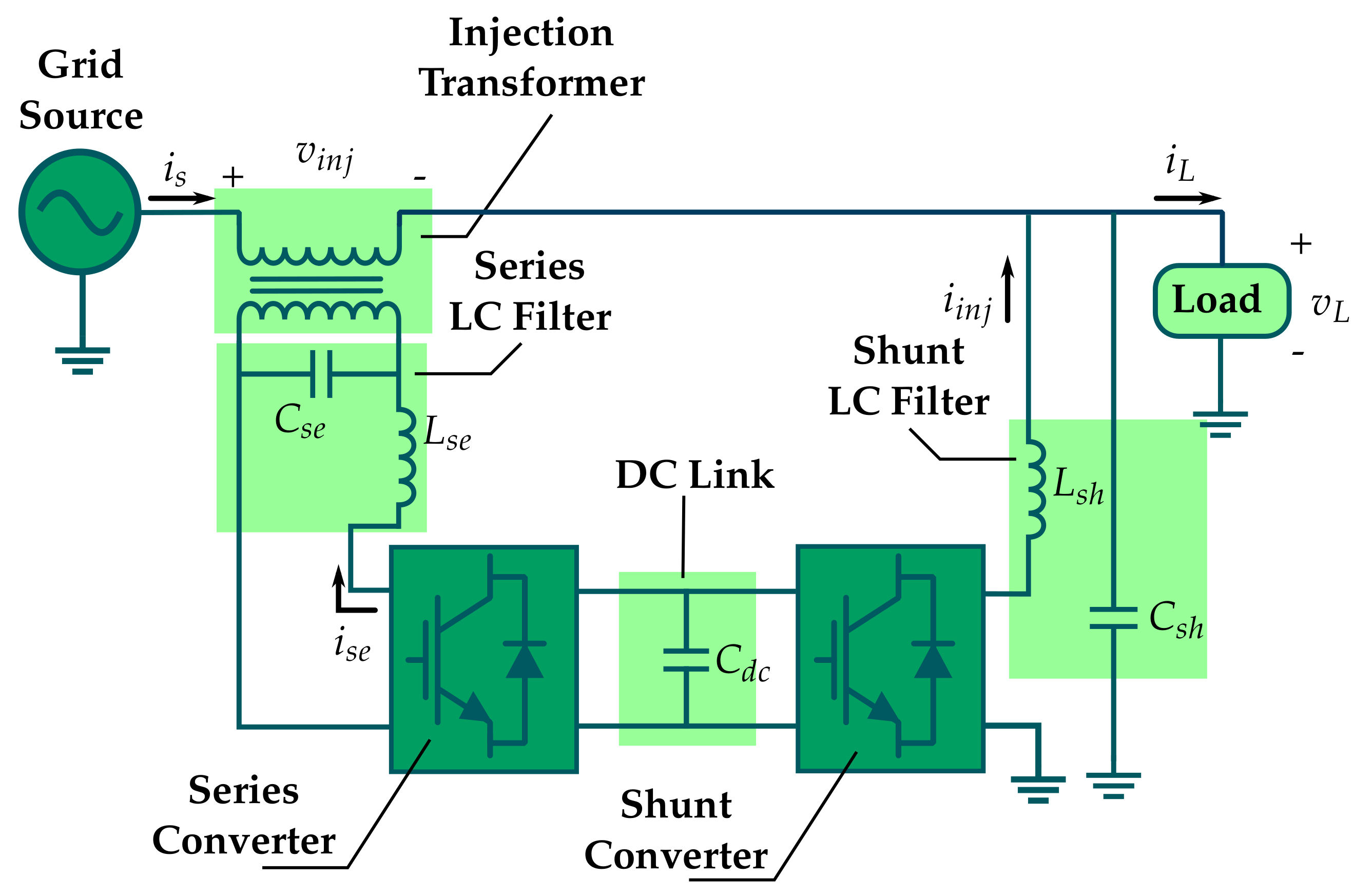
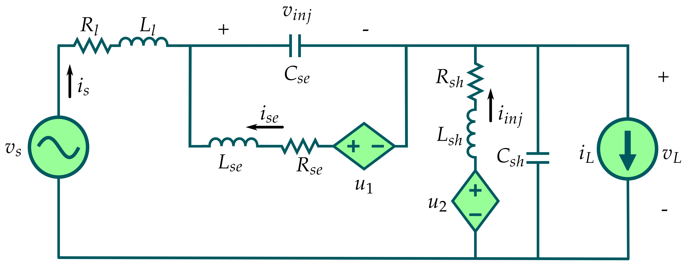
2. System Model Description

This section explains the dynamic model of the UPQC with coupling effects and DC-link dynamics considerations. The first subsection describes the UPQC continuous-time model based on conventional circuit analysis. The second subsection describes the MIMO discrete-time model with an input delay with consideration of a constant-voltage DC link. The third subsection depicts a separate DC-link discrete-time model such that these dynamics can be considered in the control system design. The last subsection discusses the necessary key points to suitably select the sampling time for the discrete models.

2.1. UPQC Stages and Continuous-Time Model

Figure 1 depicts the main stages of the UPQC. This system consists of three main parts: the series converter, which has DVR features (compensates all grid voltage variations); the shunt converter (compensates current harmonics like an active filter); and the DC link. Both power converters have LC filters to ensure smooth injected current and voltage to the grid. Furthermore, the UPQC has an injection transformer that isolates the DC-;ink nodes from the grid to avoid short circuits, as described in [20]. The main DC link feature is to keep an energy balance for the entire system. The shunt converter maintains a constant value for the DC link.

The UPQC compensates the grid voltage disturbances to provide suitable load voltage. Additionally, the load current is compensated to achieve a desired grid current. Thus, following the Kirchhoff laws based on Figure 1, the main compensation equations are:

$$\begin{array}{c}{v}_L(t)=v_s(t)-v_{inj}(t)\\ \\ i_s(t)=i_L(t)-i_{inj}(t),\end{array}$$

(1)

where the compensated load voltage $v_L\left(t\right)$ is based on the disturbed-grid voltage $v_s\left(t\right)$ and the UPQC injected voltage $v_{inj}\left(t\right)$. The grid current $i_s\left(t\right)$ depends on the disturbed load current $i_L\left(t\right)$ and the shunt converter injected current $i_{inj}\left(t\right)$. In addition, the UPQC has a series converter current $i_{se}\left(t\right)$.

To construct a dynamic model, the grid-tied UPQC is transformed to an equivalent model, as depicted in Figure 2 [21]. As the UPQC should compensate for PQ disturbances in most connected loads, the disturbances are modeled as uncertain independent current sources. The parameters of the series LC filter are the filter inductance $L_{se}$, the inductor loss resistance $R_{se}$, and the filter capacitance $C_{se}$. The shunt converter has similar parameters for its LC filter: $L_{sh}$, $R_{sh}$, and $C_{sh}$. The line inductance and the line resistance, $L_l$ and $R_l$, respectively, describe the grid losses and represent a simplified equivalent model for the injection transformer. The transformer has a ratio of 1:1 so that the series LC filter parameters do not change due to impedance transformations.

Subsequently, applying the Kirchhoff laws to the equivalent circuit and transforming the resulting equations in state space, the continuous-time UPQC model results in

$$\left\{\begin{array}{cc}\hfill {\dot{\mathbf{x}}}_c\left(t\right)& ={\mathbf{A}}_c{\mathbf{x}}_c\left(t\right)+{\mathbf{B}}_c\mathbf{u}\left(t\right)+{\mathbf{E}}_c\delta \left(t\right)\hfill \\ \hfill \mathbf{y}\left(t\right)& ={\mathbf{C}}_c{\mathbf{x}}_c,\left(t\right)\hfill \end{array}\right.$$

(2)

with

$${\mathbf{A}}_c=\left[\begin{array}{ccccc}-\frac{R_l}{L_l}& 0& 0& -\frac{1}{L_l}& -\frac{1}{L_l}\\ 0& -\frac{R_{se}}{L_{se}}& 0& -\frac{1}{L_{se}}& 0\\ 0& 0& -\frac{R_{sh}}{L_{sh}}& 0& -\frac{1}{L_{sh}}\\ \frac{1}{C_{se}}& \frac{1}{C_{se}}& 0& 0& 0\\ \frac{1}{C_{sh}}& 0& \frac{1}{C_{sh}}& 0& 0\end{array}\right],{\mathbf{B}}_c=\left[\begin{array}{cc}0& 0\\ \frac{1}{2L_{se}}& 0\\ 0& \frac{1}{2L_{sh}}\\ 0& 0\\ 0& 0\end{array}\right],{\mathbf{E}}_c=\left[\begin{array}{cc}\frac{1}{L_l}& 0\\ 0& 0\\ 0& 0\\ 0& 0\\ 0& -\frac{1}{C_{sh}}\end{array}\right],$$

$${\mathbf{C}}_c=\left[\begin{array}{ccccc}0& 0& 0& 0& 1\\ 1& 0& 0& 0& 0\end{array}\right].$$

The state matrix is ${\mathbf{A}}_c$, the input matrix is ${\mathbf{B}}_c$, the output matrix is ${\mathbf{C}}_c$, and the state disturbance matrix is ${\mathbf{E}}_c$. So, the continuous-time model has an order of $n_c=5$, a number of inputs $p=2$, a number of outputs $q=2$, and two state disturbances. The state vector for this model is ${\mathbf{x}}_c={\left[\begin{array}{ccccc}{i}_s& i_{se}& i_{inj}& v_{inj}& v_L\end{array}\right]}^T$. The output of the continuous-time model (which has the controlled variables) is described by the vector $\mathbf{y}\left(t\right)={\left[\begin{array}{cc}{v}_L\left(t\right)& i_s\left(t\right)\end{array}\right]}^T$.

The input vector is defined as $\mathbf{u}\left(t\right)={\left[\begin{array}{cc}{u}_1\left(t\right)& u_2\left(t\right)\end{array}\right]}^T$ and describes the voltage control signals that supply each power converter (modeled as dependent voltage sources in Figure 2) to achieve suitable injected current and voltage. The power converters are controlled through PWM (whose control variable is the duty cycle $d\left(t\right)$). Then, the relationship between the control signals and the power converter duty cycles using an unipolar switching is

$$d_i\left(t\right)=\frac{1}{v_{dc}\left(t\right)}\left|u_i\left(t\right)\right|=\left|{\mu }_i\left(t\right)\right|,$$

(3)

where ${\mu }_i\left(t\right)$ is defined as an averaged PWM input signal and has amplitude limits on the interval $\left[\begin{array}{cc}-1& 1\end{array}\right]$. The input voltages applied to the equivalent circuit in Figure 2 are defined as $u_i\left(t\right)={\mu }_i{V}_{dc}$, with the parameter $V_{dc}$ as the constant voltage of the DC link based on the approximation $v_{dc}\left(t\right)\approx V_{dc}$. The DC link voltage is approximated as a constant in this continuous-time model (despite the DC capacitor dynamics in this stage that produce a variable $v_{dc}\left(t\right)$), to maintain an LTI model for the UPQC. So, the control signals of $\mathbf{u}\left(t\right)$ depend directly on the DC link constant value and have amplitude limits in the interval $\left[\begin{array}{cc}-V_{dc}& V_{dc}\end{array}\right]$. The numerical value of $V_{dc}$ is shown in

Table 1. Values for the parameters used in the UPQC experimental setup.

Category	Parameter	Symbol	Value
UPQC parameters	Line Inductance	$L_l$	700 $\mathsf{\mu }$H
	Line Resistance	$R_l$	2 $\mathsf{\Omega }$
	Filters inductance	$L_{se}$; $L_{sh}$	1.365 mH
	Filters resistances	$R_{se}$; $R_{sh}$	0.85 $\mathsf{\Omega }$
	Filters capacitance	$C_{se}$; $C_{sh}$	40 $\mathsf{\mu }$F
System parameters	DC link equivalent capacitance	$C_{dc}$	1.88 mF
	DC link desired voltage	$V_{dc}$	220 V
	$v_L$ and $v_s$ voltage amplitude	$V_L^{*}$; $V_s$	110 ${\mathrm{V}}_{\mathrm{RMS}}$
	Fundamental frequency	$f_0$	60 Hz
	Sampling Frequency	$f_m$	10.2 KHz
	Switching frequency	$f_s$	18 KHz
	Number of resonators	$h_v$; $h_i$	7
	delay samples	$\tau$	2
Tuning values	${\mathbf{Q}}_o$ tuning value	$\alpha$	0.0001
	UPQC states weighing value	a	10
	UPQC delay states weighting value	b	2
	Weighting value for the resonators	$\gamma$	0.001
	error vector $\mathbf{e}(k)$ weighting value	$\epsilon$	0.1
	state feedback states weighting value	$\rho$	5
	Control signal weighting value	$\nu$	10
	Proportional value for the PI control	P	0.1184
	Integral value for the PI control	I	0.2239

.

Both the grid voltage $v_s\left(t\right)$ and the load current $i_L\left(t\right)$ are assumed to be sinusoidal signals with odd harmonics and are embedded in a disturbance vector $\delta \left(t\right)$ as follows:

$$\delta \left(t\right)=\left[\begin{array}{c}{v}_s\left(t\right)\\ i_L\left(t\right)\end{array}\right]=\left[\begin{array}{c}{V}_{s}sin\left({\omega }_{o}k+\varphi \right)+{\displaystyle \sum _{i=2}^{\infty }}{V}_{i}sin\left(\left(2i-1\right){\omega }_{0}k+{\varphi }_i\right)\\ I_{L}sin\left({\omega }_{o}k+{\varphi }_2\right)+{\displaystyle \sum _{i=2}^{\infty }}{I}_{j}sin\left(\left(2j-1\right){\omega }_{0}k+{\varphi }_j\right)\end{array}\right],$$

(4)

with ${\omega }_0$ as the fundamental grid frequency. The UPQC model considers odd harmonic-based disturbances because they are the most common components that appear in a grid-load system, as explained in [22] for current harmonics (given by linear and nonlinear loads) and [23] for voltage harmonics.

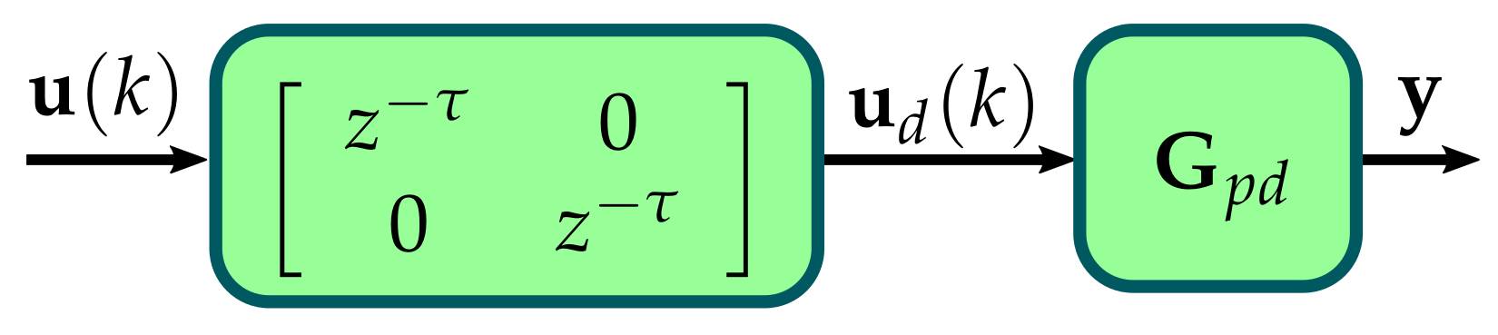
2.2. UPQC Discrete-Time System Model

After defining the continuous-time model, a zero-order hold (ZOH) approximation is applied according to the infinite series method based on [24]:

$$\begin{array}{cc}\hfill {\mathbf{A}}_d& =e^{{\mathbf{A}}_c{T}_m}={\displaystyle \sum _{i=0}^{\infty }}\frac{1}{i!}{\mathbf{A}}_c^i{T}_m^i\hfill \\ \hfill {\mathbf{B}}_d& =\left({\int }_0^{T_m}{e}^{{\mathbf{A}}_c\alpha }d\alpha \right){\mathbf{B}}_c=\left({\displaystyle \sum _{i=0}^{\infty }}\frac{T_m^{i+1}}{\left(i+1\right)!}{\mathbf{A}}_c^i\right){\mathbf{B}}_c\hfill \\ \hfill {\mathbf{E}}_d& =\left({\int }_0^{T_m}{e}^{{\mathbf{A}}_c\alpha }d\alpha \right){\mathbf{E}}_c=\left({\displaystyle \sum _{i=0}^{\infty }}\frac{T_m^{i+1}}{\left(i+1\right)!}{\mathbf{A}}_c^i\right){\mathbf{E}}_c,\hfill \end{array}$$

(5)

where the time is approximated as $t=k{T}_m$, k is the sample number, and $T_m$ is the sampling period. The discrete-time state-space matrices are defined with the subscript d. The infinite series approximation is achieved through numeric solvers. The output matrix remains equal using the aforementioned discretization method. Then, the resulting discrete-time model of the UPQC is

$${\mathbf{G}}_{pd}=\left\{\begin{array}{cc}\hfill {\mathbf{x}}_d\left(k+1\right)& ={\mathbf{A}}_d{\mathbf{x}}_d\left(k\right)+{\mathbf{B}}_d\mathbf{u}\left(k-\tau \right)+{\mathbf{E}}_d\delta \left(k\right)\hfill \\ \hfill \mathbf{y}\left(k\right)& ={\mathbf{C}}_c{\mathbf{x}}_d\left(k\right),\hfill \end{array}\right.$$

(6)

where an input delay is included due to the dynamics of the PWM interfaces used in the experimental setup. The time delay is depicted as a sample-integer number $\tau$ and is considered equal for both PWM interfaces in each power converter. Moreover, the input-time delay can be represented as a different system ${\mathbf{G}}_{ret}$ connected to the input port of the UPQC model, as shown in Figure 3. Here, the UPQC system is considered as ${\mathbf{G}}_{pd}$ and the vector ${\mathbf{u}}_d\left(k\right)$ is the output of the delay system.

Then, the state-space representation of the time-delay system is defined as

$$\begin{array}{cc}\hfill {\mathbf{x}}_{ret}\left(k+1\right)& =\underset{{\mathbf{A}}_t}{\underbrace{\left[\begin{array}{cc}{\mathbf{A}}_{ret}& \mathbf{0}\\ \mathbf{0}& {\mathbf{A}}_{ret}\end{array}\right]}}\underset{{\mathbf{x}}_t}{\underbrace{\left[\begin{array}{c}{\mathbf{x}}_{ret}\left(k\right)\\ {\mathbf{x}}_{ret}\left(k\right)\end{array}\right]}}+\underset{{\mathbf{B}}_t}{\underbrace{\left[\begin{array}{cc}{\mathbf{b}}_{ret}& \mathbf{0}\\ \mathbf{0}& {\mathbf{b}}_{ret}\end{array}\right]}\mathbf{u}\left(k\right)}\hfill \\ \hfill {\mathbf{u}}_d\left(k\right)& =\underset{{\mathbf{C}}_t}{\underbrace{\left[\begin{array}{cc}{\mathbf{c}}_{ret}& \mathbf{0}\\ \mathbf{0}& {\mathbf{c}}_{ret}\end{array}\right]}}\left[\begin{array}{c}{\mathbf{x}}_{ret}\left(k\right)\\ {\mathbf{x}}_{ret}\left(k\right)\end{array}\right],\hfill \end{array}$$

(7)

with ${\mathbf{A}}_{ret}=\left[\begin{array}{cc}{\mathbf{0}}_r& 0\\ {\mathbf{I}}_r& {\mathbf{0}}_r^{\mathrm{T}}\end{array}\right]\in {\mathbb{R}}^{\tau ,\tau }$, ${\mathbf{0}}_r\in {\mathbb{R}}^{1,\left(\tau -1\right)}$, ${\mathbf{I}}_r=\mathbf{I}\in {\mathbb{R}}^{\left(\tau -1\right),\left(\tau -1\right)}$, ${\mathbf{b}}_{ret}=\left[\begin{array}{ccc}1& 0& 0\end{array}\right.$${\left.\begin{array}{cc}\cdots & 0\end{array}\right]}^{\mathrm{T}}\in {\mathbb{R}}^{\tau ,1}$, ${\mathbf{c}}_{ret}=\left[\begin{array}{ccccc}0& 0& 0& \cdots & 1\end{array}\right]$$\in {\mathbb{R}}^{1,\tau }$ and ${\mathbf{x}}_{ret}=\left[\begin{array}{cc}{x}_1\left(k\right)& x_2\left(k\right)\end{array}\right.$${\left.\begin{array}{ccc}{x}_3\left(k\right)& \cdots & x_{\tau }\left(k\right)\end{array}\right]}^{\mathrm{T}}$. Using the block reduction in Figure 3, the UPQC discrete-time model with implicit input delay results in

$$\mathbf{G}=\left\{\begin{array}{cc}\hfill \underset{\mathbf{x}\left(k+1\right)}{\underbrace{\left[\begin{array}{c}{\mathbf{x}}_d\left(k+1\right)\\ {\mathbf{x}}_t\left(k+1\right)\end{array}\right]}}& =\underset{\mathbf{A}}{\underbrace{\left[\begin{array}{cc}{\mathbf{A}}_d& {\mathbf{B}}_d{\mathbf{C}}_t\\ {\mathbf{0}}_a& {\mathbf{A}}_t\end{array}\right]}}\underset{\mathbf{x}\left(k\right)}{\underbrace{\left[\begin{array}{c}{\mathbf{x}}_d\left(k\right)\\ {\mathbf{x}}_t\left(k\right)\end{array}\right]}}+\underset{\mathbf{B}}{\underbrace{\left[\begin{array}{c}{\mathbf{0}}_b\\ {\mathbf{B}}_t\end{array}\right]}}\mathbf{u}\left(k\right)+\underset{\mathbf{E}}{\underbrace{\left[\begin{array}{c}{\mathbf{E}}_d\\ {\mathbf{0}}_{\delta }\end{array}\right]}}\delta \left(k\right)\hfill \\ \\ \hfill \mathbf{y}\left(k\right)& =\underset{\mathbf{C}}{\underbrace{\left[\begin{array}{cc}{\mathbf{C}}_c& {\mathbf{0}}_s\end{array}\right]}}\left[\begin{array}{c}{\mathbf{x}}_d\left(k\right)\\ {\mathbf{x}}_t\left(k\right)\end{array}\right].\hfill \end{array}\right.$$

(8)

The dimensions for the zero matrices are defined as ${\mathbf{0}}_a\in {\mathbb{R}}^{2\tau ,n_c}$, ${\mathbf{0}}_b\in {\mathbb{R}}^{n_c,2}$, ${\mathbf{0}}_{\delta }\in {\mathbb{R}}^{2\tau ,2}$ and ${\mathbf{0}}_s\in {\mathbb{R}}^{2,2\tau }$. The entire system order is $n=n_c+p\tau$. The system with input delays is considered as an augmented model with the states of both the UPQC and the time-delay system. This scheme has the main advantage that the control design can be applied to a non-explicit delay model.

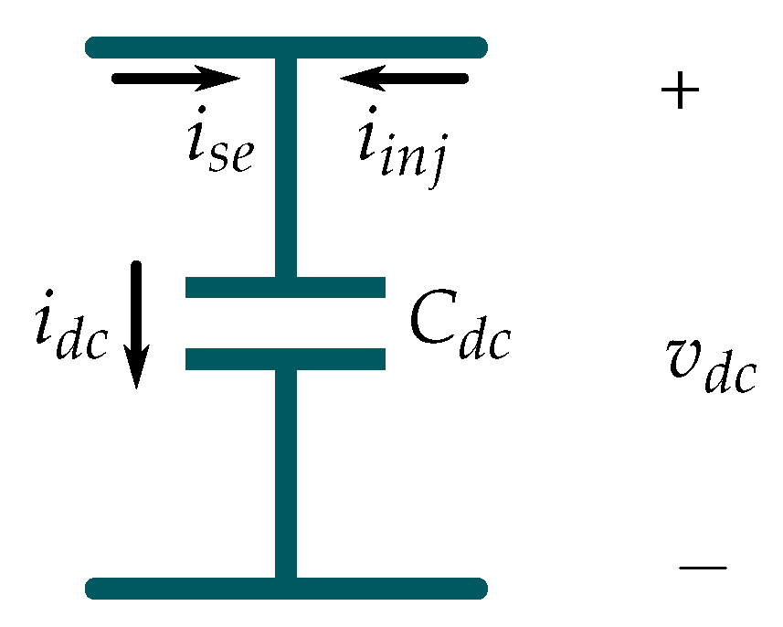
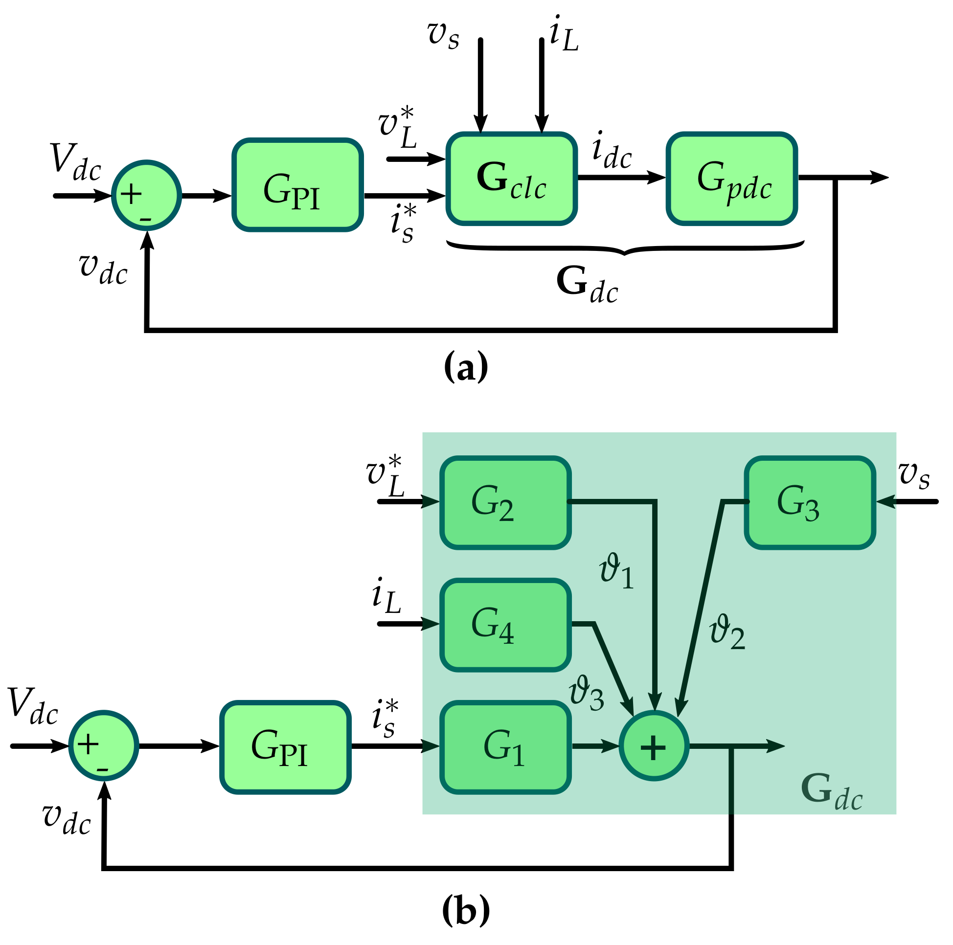
2.3. DC-Link Discrete-Time Model

As shown in the previous section, the DC link voltage in the UPQC model is considered as a constant value to avoid a nonlinear model. However, in the experimental setup, this stage is a capacitor that has associated dynamics. Considering the node analysis based on Figure 4 and the ZOH method, the discrete-time dynamics of the DC link are

$$G_{pdc}=\left\{\begin{array}{cc}\hfill v_{dc}\left(k+1\right)& =v_{dc}\left(k\right)+\frac{T_m}{C_{dc}}{i}_{dc}\left(k\right)\hfill \\ \hfill y_{dc}\left(k\right)& =v_{dc}\left(k\right),\hfill \end{array}\right.$$

(9)

where the DC link current is defined as $i_{dc}\left(k\right)=i_{se}\left(k\right)+i_{inj}\left(k\right)$ and $C_{dc}$ is the capacitance of the DC link. The sampling period for this model is considered equal to the UPQC.

2.4. Sampling Period Selection

The discrete-time model eigenvalues (whose imaginary part must be less than $\pi /T_m$) are the main criteria to choose the sampling period [24]. Additionally, this selection is related to both the cutoff frequency of the LC filters and the switching method applied to the power converters. For this case, a unipolar switching method is used based on the reduced harmonic content of the power converters compared with the bipolar technique [25]. This switching method assures that the LC filters can attenuate switching harmonics with high reliability. Therefore, as the cutoff frequency of an LC filter is given by $f_c=1/\sqrt{LC}$, a recommended criterion to achieve an attenuation higher than 40 dB for the switching harmonics is $f_s\ge 5f_c$.

According to [26,27], the recommended sampling period for the discrete-time models should be equal to the switching frequency on the PWM interfaces ($f_m=1/T_m=f_s$). However, the recommendation by [26,27] considers the measurement and sampling of unfiltered signals. If the measured and sampled signals of the control system are filtered (on the LC filters outputs), the sampling frequency could be less than the switching frequency. However, if $f_m\ll f_s$, an aliasing effect takes place on the sampled and measured signals, while an oversampling with $f_m>f_s$ causes unnecessary digital platform CPU usage. Consequently, the feedback controller could not be supported. Therefore, if ${\mathsf{\Lambda }}_c$ is the largest imaginary part of all the eigenvalues of the continuous-system model, the criterion to choose the sampling frequency should be

$$\frac{{\mathsf{\Lambda }}_c}{\pi }<f_m\le f_s,$$

(10)

and the resulting discrete-time model will have the imaginary part of the eigenvalues in the interval $\left[\begin{array}{cc}-\frac{\pi }{T_m}& \frac{\pi }{T_m}\end{array}\right]$.

3. Control System Design

This section explains the feedback control system design based on specific control objectives and an observer-based architecture. The first subsection outlines the control system objectives. The second subsection describes the control system architecture with details for each stage. The third subsection describes the tuning and design of the resonant MIMO observer. The fourth subsection explains state feedback control based on an LQR tuning and design method. The fifth subsection provides details of the UPQC control law and some technical requirements to achieve the desired closed-loop performance. The last subsection describes a proportional-integral (PI) compensator design to achieve a constant voltage in the DC link stage.

3.1. Control Objectives

Based on the IEEE-1159-2019 standard, PQ issues could be compensated if the following objectives are assured in the closed loop:

• The feedback control must track desired pure sinusoidal reference signals so that the grid current and the load voltage can be free-distorted. Similarly, as the disturbance vector $\delta \left(k\right)$ causes harmonic content on the controlled variables, the feedback control system must reject the grid voltage and the load current. According to the IEEE-519-2014 standard, the THD index for the voltage and the current (with low current consumption on the common connectionpPoint) must achieve the condition:

  $$\mathrm{THD}=\frac{\sqrt{{\displaystyle \sum _{i=2}^{\infty }}{F}_i{}^2}}{F_1}·100\%\le 5\%,$$

  (11)

  where F depicts either a voltage or a current signal. $F_i$ is the magnitude for the ith harmonic and $F_1$ is the magnitude of the fundamental component.
• The power factor on the grid side must be 1. Therefore, the reference vector $\mathbf{r}\left(k\right)$ is defined with the variable $\varphi$ as the grid voltage phase. The load voltage should have the same phase as $v_s$ to avoid phase jumps in loads. The current reference $i_s^{*}$ must have the same phase of $v_s$ to achieve the desired power factor correction. The parameter $f_0$ is the grid fundamental frequency. As a result, the reference signals are defined as

  $$\mathbf{r}\left(k\right)=\left[\begin{array}{c}{v}_L^{*}\left(k\right)\\ i_s^{*}\left(k\right)\end{array}\right]=\left[\begin{array}{c}{V}_L^{*}sin\left(2\pi f_{0}k+\varphi \right)\\ I_s^{*}sin\left(2\pi f_{0}k+\varphi \right)\end{array}\right].$$

  (12)
• The control system must achieve the steady state in a time less than a half sinusoidal cycle. This condition assures that the sags and swells will be imperceptible on the connected load according to the definition of a sag or swell in the IEEE-1159-2019 standard. Defining the settling time of the control system as $t_{ss}$, the transient time objective should be

  $$t_{ss}\le \frac{1}{2f_0}.$$

  (13)
  Similarly, during a sag or swell event, the load voltage amplitude must be in the interval of $0.9\le \frac{V_L}{V_L^{*}}\le 1.1$ following the same IEEE standard.
• To avoid saturation in the PWM interfaces, the control signals $u_i\left(k\right)$ must not exceed the interval limit $\left[\begin{array}{cc}-V_{dc}& V_{dc}\end{array}\right]$ (Table 1 lists the numerical value of $V_{dc}$). For the case of ${\mu }_i\left(k\right)$, the available magnitude is within $\left[\begin{array}{cc}-1& 1\end{array}\right]$.
• The DC-link voltage must remain at a constant voltage $V_{dc}$ and the settling time for this stage should be 10 to 100 times lower than $t_{ss}$ [28]. It implies that the DC-link variations due to transient events could be seen as static in the UPQC closed-loop dynamics.

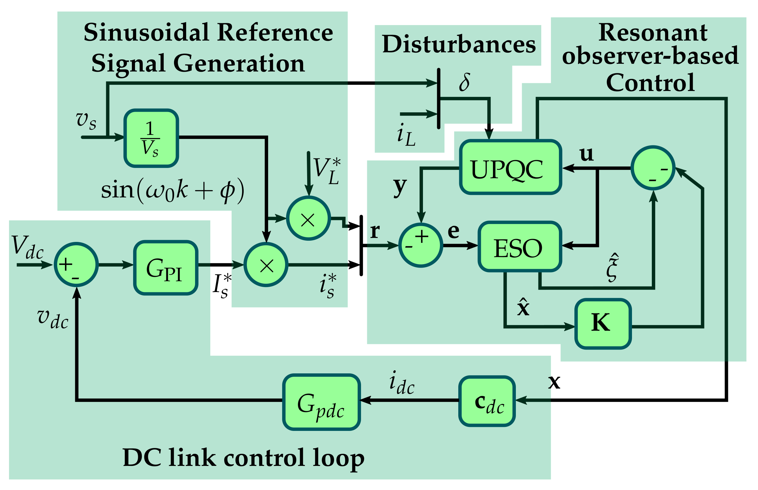
3.2. Control Architecture

There are many control architectures, as proposed in [29], which use a robust output-feedback approach to achieve the mentioned control objectives. However, this work proposes an observer-based approach with a discrete-time model description, so that a direct estimation and rejection of the coupled disturbances could be applied in the control law. The proposed control system architecture is shown in Figure 5. As the UPQC model is entirely controllable and observable, the state disturbance $\delta \left(k\right)$ could be transformed to an equivalent input disturbance $\xi \left(k\right)$ that is added to the control input $\mathbf{u}\left(k\right)$. The extended state observer (ESO) can estimate both the UPQC states and the input equivalent disturbance $\xi \left(k\right)$. If the estimated disturbance $\widehat{\xi }\left(k\right)$ is close to $\xi \left(k\right)$, it could be subtracted directly on the UPQC input port to achieve disturbance rejection.

The ESO features reference tracking if the observer input is the error vector defined as $\mathbf{e}\left(k\right)=\mathbf{y}\left(k\right)-\mathbf{r}\left(k\right)$ instead of $\mathbf{y}\left(k\right)$. This characteristic is associated with a regulation control law that leads the plant states to the equilibrium point, such that the tracking depends only on the observer dynamics. Thus, an estimated state feedback design results in the matrix $\mathbf{K}$ to achieve that regulation.

The DC link is related to the UPQC through the output vector ${\mathbf{c}}_{dc}$, where a sum between the states $i_{se}\left(k\right)$ and $i_{inj}\left(k\right)$ is performed to obtain the DC-link current $i_{dc}\left(k\right)$. Next, using the capacitor dynamics in (9), $v_{dc}\left(k\right)$ is controlled through the PI compensator to track the desired constant value $V_{dc}$. In addition, the PI control signal corresponds to the grid current reference magnitude, and it is multiplied by the grid-voltage-based unitary sine wave to achieve the sinusoidal grid current reference $i_s^{{}^{*}}\left(k\right)$. This nonlinear operation of the DC link control loop performs an energy balance on the grid-tied UPQC.

In conclusion, the control system design for the proposed scheme consists of tuning the ESO, the state feedback matrix $\mathbf{K}$, and the PI control of the DC link.

3.3. Resonant Extended State Observer Design

The extended observer must have the disturbance model in its design. Both the reference and the disturbance vector can be described through the same disturbance model since they are sinusoidal signals. One method to represent sinusoidal signals involves using repetitive control, as in [30,31], but it implies a very high system order of the closed loop. Another option, is the use of resonators which could be applied to estimate sinusoidal components. According to [32], the discrete-time representation of a single resonator is

$$\begin{array}{cc}\hfill \left[\begin{array}{c}{x}_{r1}\left(k+1\right)\\ x_{r2}\left(k+1\right)\end{array}\right]& =\underset{{\mathbf{A}}_R}{\underbrace{\left[\begin{array}{cc}cos\left(\omega T_m\right)& sin\left(\omega T_m\right)\\ -sin\left(\omega T_m\right)& cos\left(\omega T_m\right)\end{array}\right]}}\underset{{\mathbf{x}}_R}{\underbrace{\left[\begin{array}{c}{x}_{r1}\left(k\right)\\ x_{r2}\left(k\right)\end{array}\right]}}+\underset{{\mathbf{b}}_R}{\underbrace{\left[\begin{array}{c}1-cos\left(\omega T_m\right)\\ sin\left(\omega T_m\right)\end{array}\right]}}{u}_r\left(k\right)\hfill \\ \hfill y_r\left(k\right)& =\underset{{\mathbf{c}}_R}{\underbrace{\left[\begin{array}{cc}0& 1\end{array}\right]}}\underset{{\mathbf{x}}_R}{\underbrace{\left[\begin{array}{c}{x}_{r1}\left(k\right)\\ x_{r2}\left(k\right)\end{array}\right]}},\hfill \end{array}$$

(14)

and it enforces an infinite gain at a fixed frequency $\omega$, such that the observer can exactly estimate a pure sinusoidal signal of the same frequency. If the ESO must estimate several frequencies, the observer should consider several single resonators (called here a compound resonator). Based on $\delta \left(k\right)$, the control system must reject many harmonics, but the limitation is related to the closed-loop order. The system order increases two units per resonator into the ESO. If the order is higher, the control system will require more CPU usage of the digital-experimental platform. Thus, the most significant harmonics decide the resonators tuning for both $v_s$ and $i_L$.

Additionally, as the UPQC controls two variables and rejects two disturbances, different resonators must be considered for each signal type (current or voltage). Hence, the pair $v_s$ and $v_L$ will have a compound resonator, while $i_s$ and $i_L$ will have another one. Using these two compound resonators, a compact resonator is achieved with $h_v$ single resonators for the voltage and $h_i$ single resonators for the current signals. According to the control objective, the most significant frequency harmonic components decide the number of resonators to achieve a THD of less than 5%.

The frequency for each single resonator is defined as ${\omega }_j=2\pi \left(2j-1\right)f_0$ with $j\in \mathbb{N}$ and $1\le j\le h_v$ for the voltage compound resonator and $1\le j\le h_i$ for the current resonator. Hence, the compact state-space model representation of disturbances and references is

$${\mathbf{G}}_{\xi }=\left\{\begin{array}{c}\hfill {\mathbf{x}}_{\xi }\left(k+1\right)={\mathbf{A}}_{\xi }{\mathbf{x}}_{\xi }\left(k\right)\\ \hfill \xi \left(k\right)={\mathbf{C}}_{\xi }{\mathbf{x}}_{\xi }\left(k\right),\end{array}\right.$$

(15)

where the model dynamic matrix is ${\mathbf{A}}_{\xi }=\mathrm{diag}\left({\mathbf{A}}_{v1},{\mathbf{A}}_{v2},\cdots ,{\mathbf{A}}_{v{h}_v},{\mathbf{A}}_{c1},{\mathbf{A}}_{c2},\cdots ,{\mathbf{A}}_{c{h}_i}\right)$, with the subscript v or c representing either the voltage or current resonator, respectively; and ${\mathbf{A}}_{vj}$ and ${\mathbf{A}}_{cj}$ are the dynamics matrix for the jth single resonator with the same elements of ${\mathbf{A}}_R$ in (14). The output matrix is ${\mathbf{C}}_{\xi }={\left[\begin{array}{cc}{\mathbf{c}}_{\xi 1}^{\mathrm{T}}& {\mathbf{c}}_{\xi 2}^{\mathrm{T}}\end{array}\right]}^T$ with ${\mathbf{c}}_{\xi 1}=\left[\begin{array}{ccccc}{\mathbf{c}}_{v1}& {\mathbf{c}}_{v2}& \cdots & {\mathbf{c}}_{v{h}_v}& {\mathbf{0}}_{1,2h_i}\end{array}\right]$ and ${\mathbf{c}}_{\xi 2}=\left[\begin{array}{ccccc}{\mathbf{0}}_{1,2h_v}& {\mathbf{c}}_{c1}& {\mathbf{c}}_{c2}& \cdots & {\mathbf{c}}_{c{h}_i}\end{array}\right]$. The matrices ${\mathbf{c}}_{vj}$ and ${\mathbf{c}}_{cj}$ has the same structure as ${\mathbf{c}}_R$ in (14). The state vector of the disturbances and references model is ${\mathbf{x}}_{\xi }=\left[\begin{array}{cccccc}{\mathbf{x}}_{v1}& {\mathbf{x}}_{v2}& \cdots & {\mathbf{x}}_{v{h}_v}& {\mathbf{x}}_{c1}& {\mathbf{x}}_{c2}\end{array}\right.$${\left.\begin{array}{cc}\cdots & {\mathbf{x}}_{c{h}_i}\end{array}\right]}^T$ and the model order is $m=2h_v+2h_i$.

After defining the disturbance model, the extended state observer follows a Luenberger model plus the compact resonator (15), resulting in

$$\begin{array}{cc}\hfill \left[\begin{array}{c}\widehat{\mathbf{x}}\left(k+1\right)\\ {\widehat{\mathbf{x}}}_{\xi }\left(k+1\right)\end{array}\right]& =\underset{{\mathbf{A}}_{ex}}{\underbrace{\left[\begin{array}{cc}\mathbf{A}& \mathbf{B}{\mathbf{C}}_{\xi }\\ {\mathbf{0}}_1^T& {\mathbf{A}}_{\xi }\end{array}\right]}}\underset{{\mathbf{x}}_{ex}}{\underbrace{\left[\begin{array}{c}\widehat{\mathbf{x}}\left(k\right)\\ {\widehat{\mathbf{x}}}_{\xi }\left(k\right)\end{array}\right]}}+\underset{{\mathbf{B}}_{ex}}{\underbrace{\left[\begin{array}{c}\mathbf{B}\\ {\mathbf{0}}_{b\xi }\end{array}\right]}}\mathbf{u}\left(k\right)+\mathbf{L}\left[\mathbf{e}\left(k\right)-\mathbf{C}\widehat{\mathbf{x}}\left(k\right)\right]\hfill \\ \hfill \left[\begin{array}{c}\widehat{\mathbf{x}}\\ \widehat{\xi }\end{array}\right]& =\underset{{\mathbf{C}}_{ex}}{\underbrace{\left[\begin{array}{cc}\mathbf{I}& {\mathbf{0}}_1\\ {\mathbf{0}}_1^T& {\mathbf{C}}_{\xi }\end{array}\right]}}\left[\begin{array}{c}\widehat{\mathbf{x}}\left(k\right)\\ {\widehat{\mathbf{x}}}_{\xi }\left(k\right)\end{array}\right],\hfill \end{array}$$

(16)

where the observer gain matrix is defined as $\mathbf{L}={\left[\begin{array}{cc}{\mathbf{L}}_p^T& {\mathbf{L}}_{\xi }^T\end{array}\right]}^T$ with ${\mathbf{L}}_p\in {\mathbb{R}}^{q,n}$, ${\mathbf{L}}_{\xi }\in {\mathbb{R}}^{q,m}$. The zero matrices are ${\mathbf{0}}_1\in {\mathbb{R}}^{n,m}$ y ${\mathbf{0}}_{b\xi }\in {\mathbb{R}}^{m,p}$. The vector $\widehat{\mathbf{x}}\left(k\right)$ has the UPQC-estimated states and ${\widehat{\mathbf{x}}}_{\xi }\left(k\right)$ has the estimated states of the disturbances model. The observer outputs are the plant-estimated states in $\widehat{\mathbf{x}}\left(k\right)$ and the estimated coupled disturbances from the vector $\widehat{\xi }\left(k\right)$.

The ESO design results in the matrix $\mathbf{L}$ definition based on the control objectives. This matrix can be achieved through pole placement or complex optimization techniques, as shown in [33]. However, a straightforward tuning method to find a suitable design is the linear quadratic estimator (LQE), which follows the minimization of the cost function

$${\mathcal{J}}_o\left({\mathbf{x}}_{ex}\right)={\displaystyle \sum _{i=1}^{\infty }}\left[{\mathbf{x}}_{ex}^T{\mathbf{Q}}_o{\mathbf{x}}_{ex}+{\mathbf{e}}^T{\mathbf{R}}_o\mathbf{e}\right],$$

(17)

where the weighting matrix ${\mathbf{Q}}_o$ assigns bounds for the state signal amplitudes, while the matrix ${\mathbf{R}}_o$ assigns a weight for the input ones. High values of ${\mathbf{Q}}_o$ limit the amplitude of the state signals and, hence, the time response of the closed loop tends to increase. In the case of ${\mathbf{R}}_o$, high values limit the magnitude of the error vector $\mathbf{e}\left(k\right)$.

The selection of the weighting matrices for ${\mathcal{J}}_o$ can follow different strategies, such as the Kalman–Busy filter method used in [34], who used diagonal matrices for ${\mathbf{Q}}_o$ and ${\mathbf{R}}_o$. This matrix structure allows high versatility to assign different weights per state (UPQC states or resonator states) and per input signal. Therefore, ${\mathbf{Q}}_o=\mathrm{diag}\left(\begin{array}{cc}{\mathbf{Q}}_e& {\mathbf{Q}}_{\xi }\end{array}\right)$ is a block diagonal, with ${\mathbf{Q}}_e=\alpha ·\mathrm{diag}\left(\begin{array}{cccccc}a& 0.1a& 0.1a& 0.1a& a& b{\mathbf{I}}_{2\tau }\end{array}\right)$, $\alpha$, a and b are tuning parameters, and ${\mathbf{I}}_{2\tau }\in {\mathbb{R}}^{2\tau ,2\tau }$ is an identity matrix. The matrix ${\mathbf{Q}}_e$ assigns weights to each UPQC state with high penalization of the controlled variables (first and fifth state), so that the overshoots on $i_s$ and $v_L$ can be avoided. To achieve a fast response, the other UPQC states have a lower weight. The parameter b assigns a weight for the delay model states, and is assigned through iteration until the ESO results are stable.

The matrix ${\mathbf{Q}}_{\xi }$ assigns weighting values per state for the compact resonator model into the ESO. The structure of the internal model weighting matrix is ${\mathbf{Q}}_{\xi }=\left({\mathbf{I}}_2\right.$ $0.1{\mathbf{I}}_{\beta }$ ${\mathbf{I}}_{f}requency.Thefu2$$.\left.0.01{\mathbf{I}}_{\beta }\right)$, where different weights per single resonator states are assigned according to its tuned ndamental component resonator has a higher weight than the harmonics to achieve disturbance rejection. The identity matrices ${\mathbf{I}}_2$ and ${\mathbf{I}}_{\beta }$ have dimensions of $2,2$ and $\beta ,\beta$, respectively, with $\beta =\frac{m}{2}-2$ and $\gamma$ as a tuning parameter.

The input weighting matrix is defined as ${\mathbf{R}}_o=ϵ{\mathbf{I}}_2$, where one value defines the weight for both error signals in the vector $\mathbf{e}\left(k\right)$. If a low value of $ϵ$ is assigned, the ESO will have high sensitivity to noise effects in $\mathbf{y}\left(k\right)$, while a high value of this variable causes a slower transient response of the entire closed loop.

The solution for the optimization problem based on the cost function (17) consists of calculating a definite positive matrix ${\mathbf{P}}_o$ in the following Riccati equation (based on the general problem described in [24,35]):

$${\mathbf{Y}}_1-{\mathbf{P}}_o-{\mathbf{Y}}_2{\mathbf{X}}^{-1}{\mathbf{Y}}_3+{\mathbf{Q}}_o=\mathbf{0},$$

(18)

with ${\mathbf{Y}}_1={\mathbf{A}}_{ex}{\mathbf{P}}_o{\mathbf{A}}_{ex}^T$, ${\mathbf{Y}}_2={\mathbf{A}}_{ex}{\mathbf{P}}_o{\mathbf{C}}_{ex}^T$, ${\mathbf{Y}}_3={\mathbf{C}}_{ex}{\mathbf{P}}_o{\mathbf{A}}_{ex}^T$ and $\mathbf{X}={\mathbf{C}}_{ex}{\mathbf{P}}_o{\mathbf{C}}_{ex}^T+{\mathbf{R}}_o$. The gain matrix $\mathbf{L}\in {\mathbb{R}}^{\left(m+n\right),q}$ is calculated as

$$\mathbf{L}={\left({\mathbf{X}}^{-1}{\mathbf{Y}}_3\right)}^{\mathrm{T}}$$

(19)

based on the Riccatti solution matrix ${\mathbf{P}}_0$. The gain matrix achieves a regulation law so that the dynamics imposed by ${\mathbf{A}}_{ex}-\mathbf{L}{\mathbf{C}}_{ex}$ minimize the cost function ${\mathcal{J}}_o$.

3.4. State Feedback Design

The state feedback design results in the calculation of the matrix $\mathbf{K}$. Here, we use a linear quadratic regulator (LQR) algorithm based on the cost function ${\mathcal{J}}_c$, whose definition is

$${\mathcal{J}}_c\left(\mathbf{u}\right)={\displaystyle \sum _{i=1}^{\infty }}\left[{\mathbf{x}}^T{\mathbf{Q}}_c\mathbf{x}+{\mathbf{u}}^T{\mathbf{R}}_c\mathbf{u}\right].$$

(20)

By the separation principle [24], the state-feedback regulator can be designed without considering the observer. Therefore, the cost function depends on the UPQC model states and the input vector $\mathbf{u}\left(k\right)$. The state feedback control leads the states to an equilibrium point, so that $\underset{k\to \infty }{lim}\mathbf{x}\left(k\right)=\mathbf{0}$ based on $\mathbf{u}=-\mathbf{Kx}$.

The weighting matrices ${\mathbf{Q}}_c$ and ${\mathbf{R}}_c$ are diagonal, similar to the ESO design; hence, ${\mathbf{Q}}_c=\rho ·\mathrm{diag}\left(\begin{array}{cccccc}a& 0.1a& 0.1a& 0.1a& a& b{\mathbf{I}}_{2\tau }\end{array}\right)$. Empirically, we find that $\rho \ge 1000\alpha$ is a good scaling parameter for tuning the state feedback because it achieves a settling time difference between the observer and the regulator. The main idea is to obtain a faster ESO response than the stabilization law, so that the estimated states $\widehat{\mathbf{x}}\left(k\right)$ can be fed back with gain matrix $\mathbf{K}$. This criterion assures that the state feedback stabilizes the closed loop using the estimated states. The control weighting matrix is defined as ${\mathbf{R}}_c=\nu {\mathbf{I}}_2$ with $\nu \ge 1000\epsilon$, such that the stabilization law applies the suitable control signals after the ESO achieves the steady state. The solution of the optimization method for the stabilization law is related to the following Riccati equation:

$${\mathbf{U}}_1-{\mathbf{P}}_c-{\mathbf{U}}_2{\mathbf{V}}^{-1}{\mathbf{U}}_3+{\mathbf{Q}}_c=\mathbf{0},$$

(21)

with ${\mathbf{U}}_1={\mathbf{A}}^T{\mathbf{P}}_c\mathbf{A}$, ${\mathbf{U}}_2={\mathbf{A}}^T{\mathbf{P}}_c\mathbf{B}$, ${\mathbf{U}}_3={\mathbf{B}}^T{\mathbf{P}}_c\mathbf{A}$ and $\mathbf{V}={\mathbf{B}}^{\mathbf{T}}{\mathbf{P}}_{\mathbf{c}}\mathbf{B}+{\mathbf{R}}_c$. Based on the solution matrix ${\mathbf{P}}_c$ of above equation, the state feedback matrix is calculated as:

$$\mathbf{K}={\mathbf{V}}^{-1}{\mathbf{U}}_3$$

(22)

3.5. Control Law and Closed-Loop Dynamics

Using the designs for the ESO and the stabilizing matrix $\mathbf{K}$, the control law for the UPQC control system is

$$\mathbf{u}\left(k\right)=-\mathbf{K}\widehat{\mathbf{x}}\left(k\right)-\widehat{\xi }\left(k\right).$$

(23)

A good-performance closed loop is achieved if $\xi \left(k\right)\approx \widehat{\xi }\left(k\right)$, where all disturbances can be rejected appropriately and the controlled variables have a THD less than 5%. The time response $t_{ss}$ reaches the limits if the weighting matrices generate suitable eigenvalues for the matrices ${\mathbf{A}}_{ex}-{\mathbf{LC}}_{ex}$ and $\mathbf{A}-\mathbf{BK}$. Saturation is avoided with the appropriate selection of the weighting matrix ${\mathbf{R}}_c$ in the LQR algorithm because this matrix is directly related to the magnitude of the control signals $u_i\left(k\right)$.

The closed-loop dynamics yields system ${\mathbf{G}}_{cl}$ as

$${\mathbf{G}}_{cl}=\left\{\begin{array}{cc}\hfill {\mathbf{x}}_{cl}\left(k+1\right)& =\underset{{\mathbf{A}}_{cl}}{\underbrace{\left[\begin{array}{ccc}\mathbf{A}-\mathbf{BK}& \mathbf{BK}& -\mathbf{B}{\mathbf{C}}_{\xi }\\ \mathbf{0}& \mathbf{A}-{\mathbf{L}}_p\mathbf{C}& -\mathbf{B}{\mathbf{C}}_{\xi }\\ \mathbf{0}& {\mathbf{L}}_{\xi }\mathbf{C}& {\mathbf{A}}_{\xi }\end{array}\right]}}{\mathbf{x}}_{cl}\left(k\right)+\underset{{\mathbf{B}}_{cl}}{\underbrace{\left[\begin{array}{cc}\mathbf{0}& \mathbf{E}\\ {\mathbf{L}}_p& \mathbf{E}\\ -{\mathbf{L}}_{\xi }& \mathbf{0}\end{array}\right]}}\mathbf{v}\left(k\right)\hfill \\ \hfill \mathbf{y}\left(k\right)& =\left[\begin{array}{ccc}\mathbf{C}& {\mathbf{0}}_{1,n}& {\mathbf{0}}_{1,m}\end{array}\right]{\mathbf{x}}_{cl}\left(k\right),\hfill \end{array}\right.$$

(24)

with ${\mathbf{x}}_{cl}={\left[\begin{array}{ccc}\mathbf{x}& {\mathbf{e}}_o& {\widehat{\mathbf{x}}}_{\xi }\end{array}\right]}^{\mathrm{T}}$, and $\mathbf{v}={\left[\begin{array}{cc}\mathbf{r}& \delta \end{array}\right]}^{\mathrm{T}}$. The vector ${\mathbf{e}}_o\left(k\right)=\mathbf{x}\left(k\right)-\widehat{\mathbf{x}}\left(k\right)$ is the estimation error.

3.6. PI Control for DC Link

A DC link needs a control system based on the associated control objective. Therefore, a block reduction in the control scheme in Figure 5 is proposed in Figure 6 to achieve a suitably tuned PI controller.

On the basis of the ${\mathbf{G}}_{cl}$ state equation, and having a new output vector ${\mathbf{c}}_{dc}=\left[\begin{array}{cc}{\mathbf{c}}_2& {\mathbf{0}}_{dc}\end{array}\right]$ with ${\mathbf{c}}_2=\left[\begin{array}{ccccc}0& 1& 1& 0& 0\end{array}\right]$ (to obtain the $i_{dc}\left(k\right)$ value) and ${\mathbf{0}}_{dc}\in {\mathbb{R}}^{1,2\tau }$, the new system ${\mathbf{G}}_{clc}$ is defined. Subsequently, the resulting system ${\mathbf{G}}_{dc}$ from the cascade of the DC link discrete-time model $G_{pdc}$ and ${\mathbf{G}}_{clc}$ yields:

$${\mathbf{G}}_{dc}=\left\{\begin{array}{cc}\hfill \left[\begin{array}{c}{\mathbf{x}}_{cl}\left(k+1\right)\\ v_{dc}\left(k+1\right)\end{array}\right]& =\left[\begin{array}{cc}{\mathbf{A}}_{cl}& 0\\ \frac{T_m}{C_{dc}}{\mathbf{c}}_{dc}& 1\end{array}\right]\left[\begin{array}{c}{\mathbf{x}}_{cl}\left(k\right)\\ v_{dc}\left(k\right)\end{array}\right]+\left[\begin{array}{c}{\mathbf{B}}_{cl}\\ 0\end{array}\right]\mathbf{v}\left(k\right)\hfill \\ \\ \hfill y_{dc}& =\left[\begin{array}{cc}\mathbf{0}& 1\end{array}\right]\left[\begin{array}{c}{\mathbf{x}}_{cl}\left(k\right)\\ v_{dc}\left(k\right)\end{array}\right].\hfill \end{array}\right.$$

(25)

As the control output of the PI block is the magnitude of the grid current reference, the system ${\mathbf{G}}_{dc}$ has a single control input depicted as $i_s^{*}\left(k\right)$, while the other three components of $\mathbf{v}\left(k\right)$, which are $v_L^{*}\left(k\right)$, $v_s\left(k\right)$, and $i_L\left(k\right)$, are considered as state disturbances. Thus, a frequency domain reduction is proposed to achieve a plant model, such that a unity feedback control loop can be reached, as shown in Figure 6b. The frequency domain model for the state-space representation of (25) is depicted as

$$v_{dc}=G_1{i}_s^{*}+\underset{{\vartheta }_1}{\underbrace{G_2{v}_L^{*}}}+\underset{{\vartheta }_2}{\underbrace{G_3{v}_s}}+\underset{{\vartheta }_3}{\underbrace{G_4{i}_L}},$$

(26)

where $G_1$ is the transfer function from $i_s^{*}$ to the output $v_{dc}$; $G_2$, $G_3$, and $G_4$ are the transfer functions from $v_L^{*}\to v_{dc}$, $v_s\to v_{dc}$, and $i_L\to v_{dc}$, respectively. The variables ${\vartheta }_1$, ${\vartheta }_2$, and ${\vartheta }_3$ represent the effects of those disturbances on the DC-link voltage.

The PI compensator is tuned based on the analysis of the sinusoidal disturbances rejections on ${\vartheta }_1$, ${\vartheta }_2$, and ${\vartheta }_3$; the transfer function $G_1$; and the linear approximation of $i_s^{*}\approx I_s^{*}$. Thus, with classic control tuning techniques such as root locus, the approximated closed-loop eigenvalues are achieved. The main idea is that the PI controller must have low bandwidth to achieve both the slow response of the DC link and the desired attenuation of the described sinusoidal disturbances. The PI controller follows a backward Euler method:

$$G_{\mathrm{PI}}\left(z\right)=P+I\frac{T_{m}z}{z-1},$$

(27)

with P and I being the PI constants achieved with the desired tuning.

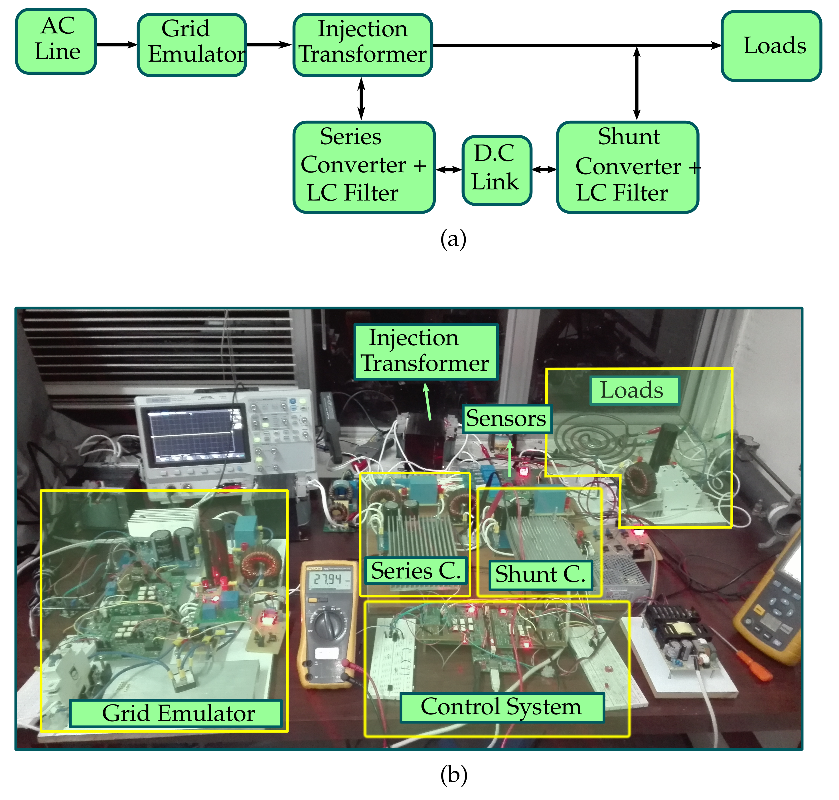
4. Experimental Setup and Results

This section describes the experimental setup and the key results, divided into harmonics compensation for the load voltage and the grid current, power factor correction (PFC) on the grid side, and grid amplitude fluctuations mitigation in the load voltage. The implementation considered a single-phase system, but the controller could be applied to three-phase systems using the Clarke stationary-frame transformation, as in [36], where the controller is the same for both the $\alpha$ and $\beta$ components.

4.1. Experimental Setup Description

The UPQC control system was implemented on the experimental setup shown in Figure 7. The experiment had a grid emulator that generated the PQ disturbances as grid voltage harmonics, sags, and swells. The grid emulator consisted of a diode bridge connected to a common AC line, a power module STK581U3C2DGEVB DC/AC converter [37], and an LC output filter. This emulator had a feedback voltage control system that was implemented with the DSP Texas Instruments Delfino C2000 TMS320F28335 (Texas Instruments; Dallas, TX, USA) [38].

The UPQC consisted of two STK581U3C2DGEVB modules: one for the series converter and the other for the shunt converter. Each power converter had output LC filters, and those were tied to the injection transformer (for the series compensation) or shunt-connected to the grid according to the circuit diagram in Figure 1. The modules STK581U3C2DGEVB had DC-link capacitors that allowed connecting both power modules back-to-back. The output LC filters are based on power toroidal inductors and polyester film capacitors to achieve good performance against harmonics, and Table 1 lists their values. The inductance values followed the identification process detailed in [20].

The overall MIMO control system for the UPQC was programmed in another DSP TMS320F28335 using the tuning parameters in Table 1 for the ESO, the state-feedback loop, and the PI controller. The digital platform acquired voltage and current signals from LEM LV25P, LA-55P, and HX10-P through a signal conditioning stage. The output PWM signals from the DSP transmitted to the power converters through a voltage-level conditioning stage.

Lastly, the experimental setup had a load connection stage for connecting different linear and nonlinear loads. In the implementation, we used this stage to analyze current disturbances caused by any load and to show the UPQC’s reactive compensation feature.

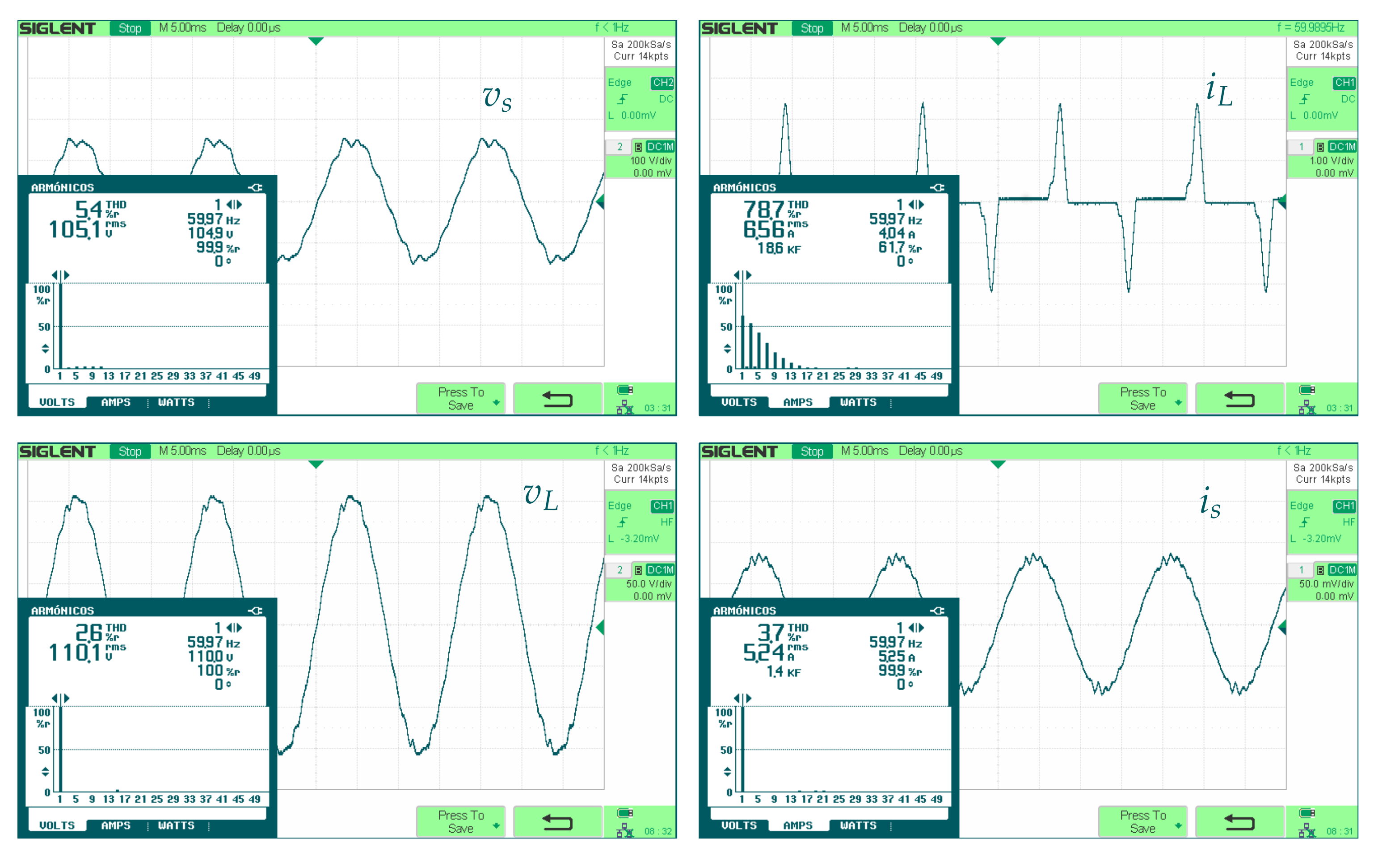
4.2. Harmonics Compensation

The main objective of the UPQC in terms of harmonic compensation is to reduce the THD index of the load voltage $v_L$ and the source current $i_s$ despite the grid voltage $v_s$ and the load current $i_L$ being highly distorted. The results shown in

Table 2. Results of harmonics compensation.

Item	Description	${\mathit{v}}_{\mathit{s}}$		${\mathit{i}}_{\mathit{L}}$		${\mathit{v}}_{\mathit{L}}$		${\mathit{i}}_{\mathit{s}}$
		THD	RMS	THD	RMS	THD	RMS	THD	RMS
		(%)	(V)	(%)	(A)	(%)	(V)	(%)	(A)
R_30	Resistive load of 30 $\mathsf{\Omega }$	10.3	102	3.1	3.78	0.8	110.1	1.2	4.9
R_50	Resistive load of 50 $\mathsf{\Omega }$	2.4	112	2	2.08	0.8	110.1	3.5	2.24
RL_30	RL load of R = 30 $\mathsf{\Omega }$ L = 35 mH	4.2	111.3	16.9	2.88	1.4	110.1	2.4	2.76
RNL_50	Nonlinear load with R = 50 $\mathsf{\Omega }$	5.4	105.4	78.7	6.56	2.6	110.1	3.7	5.24
RNL_80	Nonlinear load with R = 80 $\mathsf{\Omega }$	4.3	109.8	80.8	4.49	2.5	110.1	4.8	3.06

, with some experimental evidence in Figure 8, depict the desired harmonic compensation performance in both controlled signals. The table shows several load-changing experiments using resistive loads, RL loads, and nonlinear diode bridge-based loads with a parallel fixed capacitance and a per-experiment varying resistance. In each experiment, we applied a different kind of connected load that caused harmonic components and RMS variations in the grid emulator voltage $v_s$.

The results in Table 2 and the measured THD values in Figure 8 for the specific experiment RNL_50 show that the UPQC with the proposed controller achieves THD values below 5% for $v_L$ and $i_s$, despite the high harmonic content in the disturbed signals. In addition, the UPQC compensates for the $v_s$ amplitude to the desired RMS value on $v_L$.

According to the Table 2, the THD for the grid current increases when the load consumption lowers because this index is a relative quantity. If the fundamental value is lower, the ratio between it and the sum of the amplitude of the harmonics will be lower. Therefore, as the load impedance was high in experiments RNL_80 and R_50, both the load and the grid currents had low amplitude, and the THD increased. For the load voltage, as the fundamental amplitude was higher than the harmonics, the THD percentages were low. For the RNL_80 experiment, as the load was nonlinear and had a high impedance, the load current harmonics with frequencies higher than $(2h_i-1)f_0$ had a significant amplitude compared with the fundamental frequency and, hence, the grid current THD approached the limit.

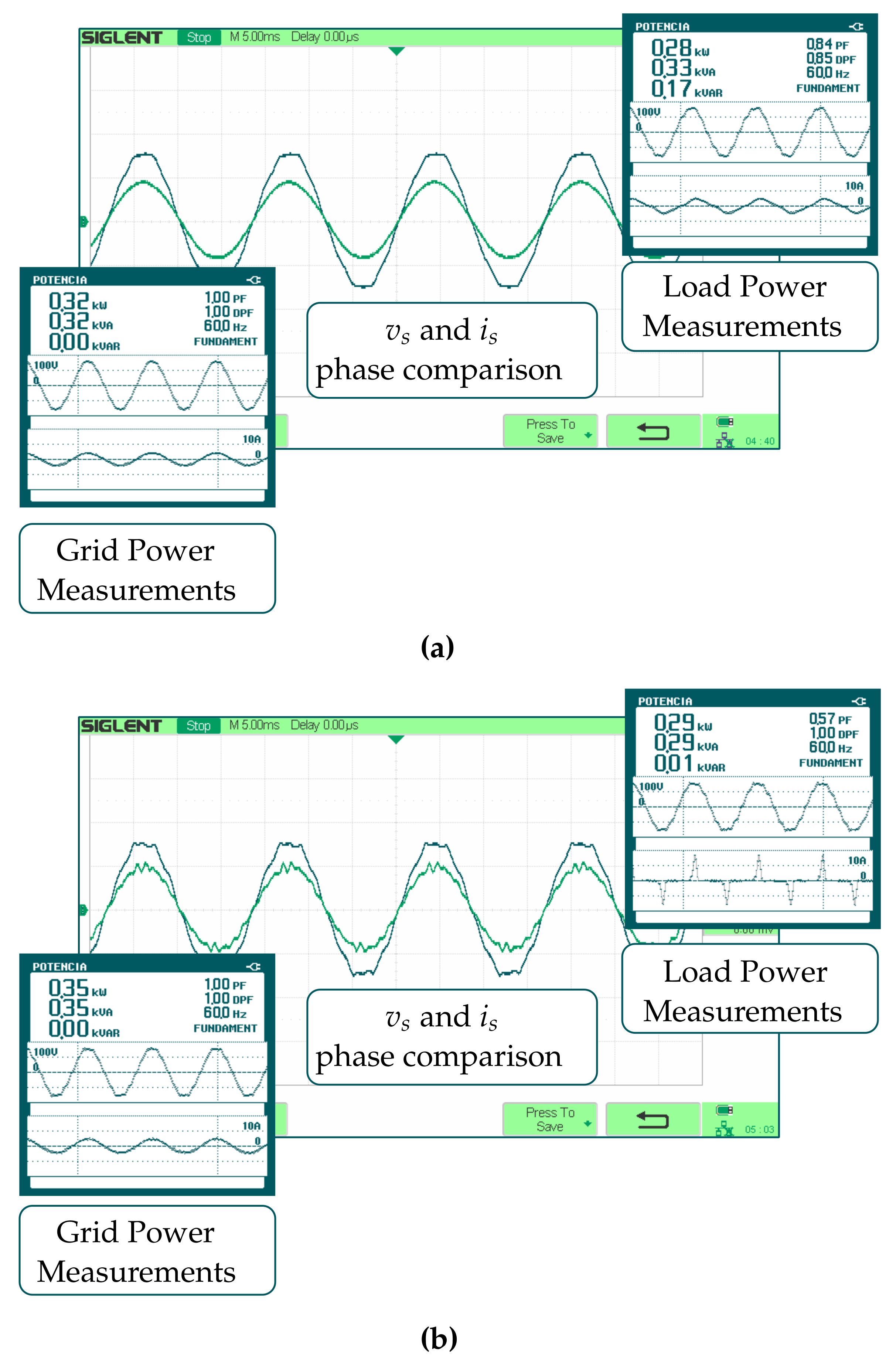
4.3. Power Factor Compensation

The UPQC can compensate for the power factor on the grid side due to $i_s^{*}$, which has the same phase and frequency as the grid voltage. A unitary power factor on the grid side avoids the reactive power flux from the load to the grid. In

Table 3. Experimental results of power factor compensation.

Item	Description	Grid		Load
		Power	PF	Power		PF
		${\mathit{P}}_{\mathit{s}}$ (W)		${\mathit{P}}_{\mathit{L}}$ (W)	${\mathit{Q}}_{\mathit{L}}$ (VAR)
R_30	Resistive Load R = 30_$\mathsf{\Omega }$	530	1	400	0	1
R_50	Resistive Load R = 50_$\mathsf{\Omega }$	260	1	230	0	1
RL_30	RL Load R = 30 $\mathsf{\Omega }$ y L = 35 mH	320	1	280	170	0.84
RL_50	RL Load R = 30 $\mathsf{\Omega }$ y L = 35 mH	210	1	180	70	0.93
RNL_50	Nonlinear load R = 50 $\mathsf{\Omega }$	580	1	411	593	0.57
RNL_80	Carga No Lineal R = 80 $\mathsf{\Omega }$	350	1	282	407	0.57

, the results show the unitary power factor on the grid side for various loads and and experiments. The table shows that the reactive power of the grid is reduced to zero, while the UPQC supplies the required $Q_L$ for connected lagging-linear or nonlinear loads. On the other hand, this effect does not occur on pure-resistive loads because they do not require reactive power from the grid. However, the power losses in the PQ compensator cause an increase in the grid active power $P_s$ compared with $P_L$. The active-power losses depended on the load impedance in each experiment, where low impedance resulted in high UPQC currents and, thus, higher power losses.

The power factor compensation is also demonstrated by the phase shift of $i_s$ and $v_s$, where it must be zero to achieve a unitary power factor. Figure 9 depicts the results of the power quality analyzer and oscilloscope, where the phase shift between the grid voltage and the grid current is zero.

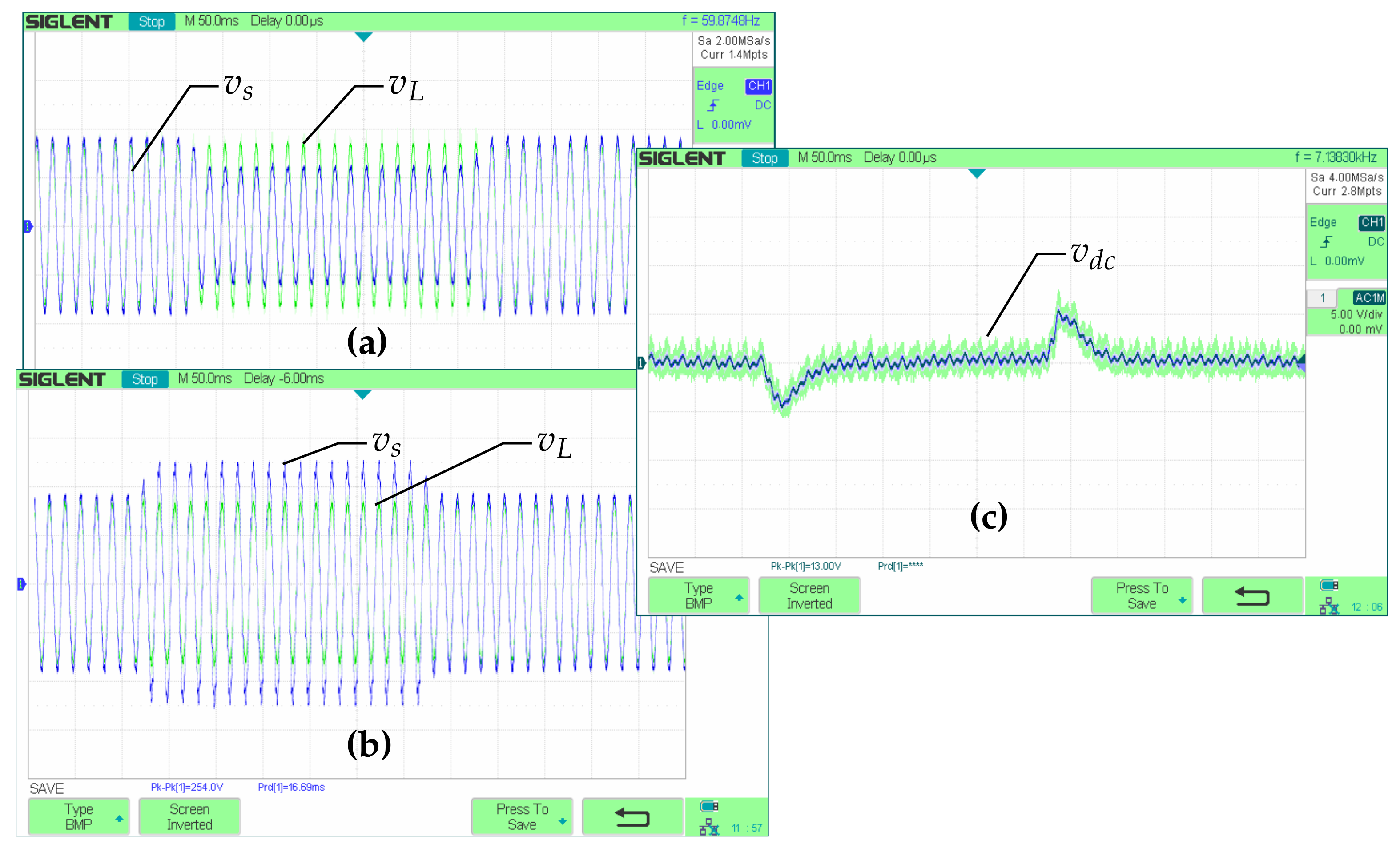
4.4. Sags and Swells Compensation

The sags and swells were tested on a resistive load of 50 $\mathsf{\Omega }$, and the sag response for the UPQC is shown in Figure 10a, where the grid emulator generated a 70% sag ($0.7V_s$). The UPQC responded within a time of $t_{ss}\approx \frac{1}{4f_0}=4$ ms, which is less than a half cycle; therefore, the control objective was achieved because $v_L$ does not change the amplitude despite the sag event on $v_s$. For the swell event, shown in Figure 10b, a 20% variation ($1.2V_s$) was applied, obtaining the desired results in terms of response time and no overshoots in the transient regimen. Here, the sags and swells had a time duration of 250 ms and showed the transients of both the event start and the recovery.

When an amplitude variation occurs in the single-phase grid, the DC link stage changes its voltage by the power flux variation in the entire system. Figure 10c shows the transient regimens of the DC link controlled by the PI stage for the sag event. The duration of the transient state for the DC link for both the event occurrence and the recovery is near to 100 ms, which is 25 times higher than the obtained $t_{ss}$. Regardless, the PI control system can recover the desired $V_{dc}$ value so that are changes neither in the DC-link voltage, nor the event compensation, nor in a normal mode.

5. Conclusions

This paper proposed a control system based on a resonant extended state observer to achieve disturbance rejection and reference tracking for sinusoidal signals using a unified power quality conditioner. As a difference from other related methods, the control system is MIMO and is based on a multivariable plant model. It helps to set the internal stability statement considering all coupling effects given among the power converters and the grid–load system. As a result, the UPQC achieves harmonics rejection for both current and voltage signals, power factor correction, and sags and swells compensation.

The input delay UPQC model is essential to design stable control systems on the experimental setup that has PWM generators with this characteristic. If the UPQC model does not consider input delays, robust stability in the closed-loop design cannot be assured. The discrete-time control design ensures accurate resonators instead of working with a continuous-time design and subsequently applying a discretization method on the closed loop.

If the number of single resonators increases in the control system, higher performance is achieved. However, the digital platform, which supports the control system implementation, limits this number of resonators. As such, the designer should choose the higher-magnitude harmonic components so that the total harmonic distortion is below 5%.

The UPQC with the proposed control system achieves harmonic compensation, providing better performance with low impedance loads. However, the proposed closed loop fulfills the control objective of avoiding harmonic distortion with a THD lower than 5% in all experiments. Similarly, the UPQC can compensate for the power factor so that the grid supplies only active power to the connected load, despite its kind. The reactive power on the grid side is zero due to PFC, while the grid active power slightly increases compared with the load active power due to the PQ compensator losses.

The control system on the UPQC achieves compensation of the voltage amplitude variations such as sags and swells with a short settling time. The transient regimen experiences no overshoots either in the event start or in the recovery. The DC link experiences mild changes in its voltage that assure UPQC stability in those variations.

The proposed closed loop shows high PQ compensation performance for the load voltage and the grid current. The control system is versatile in achieving desired transient regimens and providing the desired steady-state operation during events of harmonic distortion, sags, swells, and power factor deviations. The proposed design was verified on an experimental setup, obtaining desired results according to the IEEE standards and technical recommendations.

References

1. IEEE Standard 1159-2019—IEEE Recommended Practice for Monitoring Electric Power Quality; IEEE: New York, NY, USA, 2019; pp. 1–98.
2. Chandrasekaran, K.; Ramachandaramurthy, V. An improved Dynamic Voltage Restorer for power quality improvement. Int. J. Electric. Power Energy Syst. 2016, 82, 354–362. [Google Scholar] [CrossRef]
3. Moghassemi, A.; Padmanaban, S. Dynamic Voltage Restorer (DVR): A Comprehensive Review of Topologies, Power Converters, Control Methods, and Modified Configurations. Energies 2020, 13, 4152. [Google Scholar] [CrossRef]
4. Jiang, S.; Cui, G.; Cao, L.; Li, C. Design of H∞ robust control for single-phase shunt Active Power Filters. In Proceedings of the 2008 IEEE 7th World Congress on Intelligent Control and Automation, Chongqing, China, 25–27 June 2008; pp. 4639–4642. [Google Scholar] [CrossRef]
5. Wu, Z.; Zhang, G. Research on sliding mode control based on exact feedback linearization for single-phase shunt APF. In Proceedings of the 2016 IEEE 8th International Power Electronics and Motion Control Conference (IPEMC-ECCE Asia), Hefei, China, 22–26 May 2016; pp. 1350–1356. [Google Scholar] [CrossRef]
6. Ghosh, A.; Ledwich, G. A unified power quality conditioner (UPQC) for simultaneous voltage and current compensation. Electr. Power Syst. Res. 2001, 59, 55–63. [Google Scholar] [CrossRef]
7. Li, P.; Li, Y.; Yin, Z. Realization of UPQC H coordinated control in Microgrid. Int. J. Electr. Power Energy Syst. 2015, 65, 443–452. [Google Scholar] [CrossRef]
8. Trinh, Q.N.; Lee, H.H. Improvement of unified power quality conditioner performance with enhanced resonant control strategy. IET Gener. Transm. Distrib. 2014, 8, 2114–2123. [Google Scholar] [CrossRef]
9. Trinh, Q.N.; Lee, H.H. Versatile UPQC Control System with a Modified Repetitive Controller under Nonlinear and Unbalanced Loads. J. Power Electron. 2015, 15, 1093–1104. [Google Scholar] [CrossRef] [Green Version]
10. Tran, T.V.; Kim, K.H.; Lai, J.S. Optimized Active Disturbance Rejection Control with Resonant Extended State Observer for Grid Voltage Sensorless LCL -Filtered Inverter. IEEE Trans. Power Electron. 2021, 36, 13317–13331. [Google Scholar] [CrossRef]
11. Errouissi, R.; Shareef, H.; Awwad, F. Disturbance Observer-Based Control for Three-Phase Grid-Tied Inverter with LCL Filter. IEEE Trans. Ind. Appl. 2021, 57, 5411–5424. [Google Scholar] [CrossRef]
12. Errouissi, R.; Shareef, H.; Wahyudie, A. A Novel Design of PR Controller with Antiwindup Scheme for Single-Phase Interconnected PV Systems. IEEE Trans. Ind. Appl. 2021, 57, 5461–5475. [Google Scholar] [CrossRef]
13. Xin, Q.; Wang, C.; Chen, C.Y.; Yang, G.; Chen, L. Robust Vibration Control Based on Rigid-Body State Observer for Modular Joints. Machines 2021, 9, 194. [Google Scholar] [CrossRef]
14. Chandrakala Devi, S.; Singh, B.; Devassy, S. Modified generalised integrator based control strategy for solar PV fed UPQC enabling power quality improvement. IET Gener. Transm. Distrib. 2020, 14, 3127–3138. [Google Scholar] [CrossRef]
15. Rajendran, M. Comparison of Various Control Strategies for UPQC to Mitigate PQ Issues. J. Inst. Eng. Ser. B 2021, 102, 19–29. [Google Scholar] [CrossRef]
16. Alam, S.J.; Arya, S.R. Control of UPQC based on steady state linear Kalman filter for compensation of power quality problems. Chin. J. Electr. Eng. 2020, 6, 52–65. [Google Scholar] [CrossRef]
17. IEEE Standard 519-2014—IEEE Recommended Practice and Requirements for Harmonic Control in Electric Power Systems; IEEE: New York, NY, USA, 2014; pp. 1–29.
18. IEEE Std 1547-2018 (Revision of IEEE Standard 1547-2003). IEEE Standard for Interconnection and Interoperability of Distributed Energy Resources with Associated Electric Power Systems Interfaces; IEEE: New York, NY, USA, 2018; pp. 1–138. [Google Scholar] [CrossRef]
19. International Electrotechnical Commission. Electromagnetic Compatibility (EMC)—Part 3-2: Limits—Limits for Harmonic Current Emissions (Equipment Input Current < 16 A per phase); International Standard IEC 61000-3-2:2018 + AMD1:2020; International Electrotechnical Commission: Geneva, Switzerland, 2020. [Google Scholar]
20. Bueno-Contreras, H. Control system design of a quality power compensator. Master’s Thesis, Universidad Nacional de Colombia, Bogotá, Colombia, 2020. [Google Scholar]
21. Kwan, K.H.; Chu, Y.C.; So, P.L. Model-Based H Control of a Unified Power Quality Conditioner. IEEE Trans. Ind. Electron. 2009, 56, 2493–2504. [Google Scholar] [CrossRef]
22. Patidar, R.D.; Singh, S.P. Harmonics estimation and modeling of residential and commercial loads. In Proceedings of the 2009 IEEE International Conference on Power Systems, Kharagpur, India, 27–29 December 2009; pp. 1–6. [Google Scholar] [CrossRef]
23. Ruiz, J.; Ortiz, F. Metodologías para Identificar Fuentes Armónicas en Sistemas Eléctricos. Bachelor’s Thesis, Universidad Tecnológica de Pereira, Pereira, Colombia, 2007. [Google Scholar]
24. Chen, C.T. Analog and Digital Control System Design: Transfer-Function, State-Space, and Algebraic Methods; Oxford Series in Electrical and Computer Engineering; Saunders College Pub.: Rochester, NY, USA, 1993. [Google Scholar]
25. Lai, R.-S.; Ngo, K. A PWM method for reduction of switching loss in a full-bridge inverter. IEEE Trans. Power Electron. 1995, 10, 326–332. [Google Scholar] [CrossRef]
26. Buso, S.; Mattavelli, P. Digital Control in Power Electronics; Morgan & Claypool: San Rafael, CA, USA, 2006; Volume 1, pp. 1–158. [Google Scholar] [CrossRef] [Green Version]
27. Corradini, L.; Maksimovic, D.; Mattavelli, P.; Zane, R. Digital Control of High-Frequency Switched-Mode Power Converters; IEEE Press Series on Power Engineering; Wiley: Hoboken, NJ, USA, 2015. [Google Scholar]
28. Melo, I. Diseño, Implementación y Evaluación de Diferentes Estrategias de Control Orientadas al Rechazo Activo de Perturbaciones para un Rectificador PFC que Permitan Obtener una alta Calidad de Energía Eléctrica Medida Desde los Parámetros de PF y THD de Corrient. Master’s Thesis, Universidad Nacional de Colombia, Bogotá, Colombia, 2015. [Google Scholar]
29. Bueno-Contreras, H.; Ramos, G.A.; Costa-Castelló, R. Robust H∞ Design for Resonant Control in a CVCF Inverter Application over Load Uncertainties. Electronics 2020, 9, 66. [Google Scholar] [CrossRef] [Green Version]
30. Ramos, G.A.; Ruget, R.I.; Costa-Castelló, R. Robust Repetitive Control of Power Inverters for Standalone Operation in DG Systems. IEEE Trans. Energy Convers. 2020, 35, 237–247. [Google Scholar] [CrossRef]
31. Ramos, G.; Costa-Castelló, R. Comparison of Different Repetitive Control Architectures: Synthesis and Comparison. Application to VSI Converters. Electronics 2018, 7, 446. [Google Scholar] [CrossRef] [Green Version]
32. McGrath, B.P.; Holmes, D.G. Accurate state space realisations of resonant filters for high performance inverter control applications. In Proceedings of the 2016 IEEE 2nd Annual Southern Power Electronics Conference (SPEC), Auckland, New Zealand, 5–8 December 2016; pp. 1–6. [Google Scholar] [CrossRef]
33. Ramos, G.A.; Costa-Castelló, R.; Cortés-Romero, J. LPV Observer-Based Strategy for Rejection of Periodic Disturbances with Time-Varying Frequency. Math. Probl. Eng. 2015, 2015, 380609. [Google Scholar] [CrossRef]
34. Cortes, J.; Ramos, G.; Costa, R. Discrete-Time Resonant Observer Based Control for Periodic Signal Rejection. IEEE Lat. Am. Trans. 2015, 13, 1279–1285. [Google Scholar] [CrossRef] [Green Version]
35. Mathworks Inc. Linear-Quadratic (LQ) State-Feedback Regulator for Discrete-Time State-Space System; The MathWorks, Inc.: Natick, MA, USA, 2021. [Google Scholar]
36. Tien, D.; Gono, R.; Leonowicz, Z. A Multifunctional Dynamic Voltage Restorer for Power Quality Improvement. Energies 2018, 11, 1351. [Google Scholar] [CrossRef] [Green Version]
37. ON Semiconductor. STK581U3C2D-E Application Note. Application Note, ON Semiconductor 2014. Available online: http://www.micro-semiconductor.sg/datasheet/8f-STK581U3C2D-E.pdf (accessed on 10 October 2021).
38. Texas Instruments. TMS320x2833x, TMS320x2823x Technical Reference Manual. Tms320x2833x Datasheet. 2020. Available online: https://www.ti.com/lit/ug/sprui07/sprui07.pdf?ts=1634725545896 (accessed on 10 October 2021).
Figure 1. Stages of a UPQC for both voltage and current compensation.
Energies 14 06938 g001
Figure 2. Equivalent model of a single-phase grid-tied UPQC.
Energies 14 06938 g002
Figure 3. Input delay separation for the UPQC system model.
Energies 14 06938 g003
Figure 4. Current directions for node analysis in the DC link.
Energies 14 06938 g004
Figure 5. Resonant observer-based control scheme.
Energies 14 06938 g005
Figure 6. Closed loop system reduction to achieve PI controller tuning for the DC-link stage.
Energies 14 06938 g006
Figure 7. Experimental setup for the UPQC. (a) Block diagram for the experimental setup stages. (b) Experimental setup in the laboratory.
Energies 14 06938 g007
Figure 8. Results from a power analyzer and oscilloscope for the RNL_50 experiment of harmonics compensation.
Energies 14 06938 g008
Figure 9. Experimental results for power factor correction in (a) RL_30 and (b) RNL_80.
Energies 14 06938 g009
Figure 10. Experimental results of amplitude variations in the grid voltage: (a) sag response, (b) swell response, and (c) DC-link transient.
Energies 14 06938 g010