Abstract
Future renewable energy communities will reshape the paradigm in which we design and control efficient power systems at the district level. In this manner, the focus will be fundamentally shifted towards sustainable related concepts such as self-consumption, self-sufficiency and net energy exchanged with the grid. In this context, the paper presents a novel approach for optimally designing and controlling the photovoltaic plant and energy storage systems for a metro station in order to increase collective self-consumption and self-sufficiency at the district level. The methodology considers a community of several households connected to a subway station and focuses on the interaction between energy sources and consumers. Furthermore, the optimal solution is determined by using a Mixed Integer Linear Programming Approach, and the impact of different configurations on the overall district benefit is investigated by using several simulation scenarios. The work presents a detailed case study to underline the benefits and flexibility offered by the energy storage system in comparison with a scenario involving only a photovoltaic plant.
1. Introduction
District level energy management strategies will represent an important topic in capitalising renewable energy under the newly proposed Energy Community paradigm. In addition to the already intuitive models based on renewable energy sources sharing, new opportunities will arise in providing energy to large urban consumers (for example, metropolitan stations) during periods where the collective amount of photovoltaic production is larger then the necessary district load or through modeling flexibilities in novel manners, either by involving citizens or by using storage capabilities as a limited but controllable flexibility. From another point of view, data-driven models and data-driven control techniques are considered to be very useful instruments in this direction, and some of them are related to renewable energy integration in community life.
Since there is already an important focus at the European level [1] for energy communities, this newly presented paradigm may allow us to proceed further in the quest for obtaining net-zero carbon related energy. The novel energy community concept was introduced recently by the European Parliament in two directives, outlining the main concepts that generally describe two community types: the renewable energy community [2] and the citizen energy community [3]. This new concept is introduced as a potential emerging solution to increase the involvement of citizens in the energy market through new participation methods and, thus, stepping forwards towards reducing carbon emissions until 2030. Therefore, energy communities appear as new legal organizational forms in which citizens may join and play decisive roles such as being main shareholders in the decision process where participation is open, and the main objective is to provide environmental, social and economical benefits to the respective community. Thus, two community types are defined:
- Citizen energy communities—electricity based communities where there may be no geographical limitation;
- Renewable energy communities—limited in terms of geographical positioning, with an indirect objective to increase the share of renewable energy at the district, city and national level.
Regarding renewable energy communities, this new organisational form may represent a very attractive and interesting solution for districts. For example, citizens that have renewable energy sources deployed may join such a community and share the surplus energy with members that do not have access to renewable energy sources but want to be directly involved in community life and contribute in other ways (for example providing demand flexibility). On the other hand, since community members are the main shareholders and are directly involved in the governance of the community, they can also decide to make energy related investments with acquired profits for the benefit of the community. More specifically, if energy storage solutions were not so attractive now for singular households due to the investment cost [4] and required mounting space, such investments might be feasibly attractive for a renewable energy community.
Concepts such as collective self-consumption (SC) and individual self-consumption represent the ground platform upon which novel energy management strategies will be developed; thus, it is important to capitalize the opportunity given by the data driven instruments aforementioned in the new renewable energy framework. Since SC at individual level represents a measure of how much of the produced energy is consumed by the investigated power system, we can consider collective self-consumption at the district level to be a measure of how much produced energy at community level is internally consumed by the community. Scientifically, this concept is interesting since it allows district citizens that do not have installed renewable energy sources to join the community and increase collective self-consumption; however, dealing with surplus energy peaks still represents a challenge.
With this in mind, surplus renewable energy can be easily injected into the grid; however, in the renewable energy community framework, we distinguish several opportunities in order to increase collective self-consumption. For example, it would be interesting to investigate the impact on collective self-consumption if a district of houses gains access to available energy storage systems in order to store surplus energy during peak production hours. Another interesting idea is to integrate other urban energy consumers such as metropolitan stations in the community and to supply them with surplus renewable energy in exchange for certain benefits. Since metropolitan stations are utility-scale consumers, with limited capabilities for installing renewable energy sources, the energy community might represent a way to increase renewable energy shares relative to the energy-demanding transportation sector.
Consequently, this paper focuses on providing an investigation into an optimal control strategy for an energy storage system (ESS) for a district of houses located near a metropolitan station. The proposed method also assess the optimal sizing of the respective storage system and a connected photovoltaic (PV) plant.
A first contribution of this paper is represented by an optimisation problem that is formulated accordingly in order to provide the control strategy and sizing configuration that minimise the collective net-energy exchanged with the grid (NEEG), a novel metric. In this manner, collective self-consumption and collective self-sufficiency (SS) are maximised for the entire district. While SC defines the quantity of produced energy that is internally consumed by the system, self-sufficiency relates to how much of the system load is covered by internal energy production. The novelty not only resides in the optimisation objective, but also in the applied context where flexibility by the ESS is investigated for a potential energy community made of multiple power systems.
Another contribution is related to district modeling. As mentioned before, the aim is to conceptualize a potential energy community that is constructed from both residential homes and an urban related consumer, which is the subway station.
Performances for the proposed method are evaluated in several simulation scenarios, where the impact over collective self-consumption and collective self-sufficiency of the district is analysed for different configurations.These represent another contribution, since self-consumption is conceptually fundamental for energy communities, and self-sufficiency indicates the economical impact of the proposed management strategy. More specifically, under the assumption that the community does not obtain money from injecting energy into the grid, SS can be perceived as a measure of how much the energy bill is reduced by internal energy production (for example, if we have , then the energy bill is 50% lower).
The paper is structured in the following manner:
- Section 2 address other state-of-the-art works regarding optimal battery control, self-consumption optimisation and utility scale power systems.
- Section 3 focuses on the problem statement, emphasising the importance of criteria such as NEEG, SC and SS.
- Following the problem formulation, the power system models used in the research are presented, along with the optimisation problem.
- Section 5 presents detailed discussion over the simulation scenarios and the impact over the district collective self-consumption and self-sufficiency.
- In the final section, we present several conclusions and further research perspectives.
2. State-of-the-Art Related Works
There are many relevant works that address the optimal control of batteries in various contexts [5,6] with a focus in minimising cost with model predictive control strategies [7]; some of them use controllable and uncontrollable loads [8,9]. These works represent an interesting starting point based on the available data-related instruments and computational tools available nowadays. Comparing to works where controllable and uncontrollable loads are investigated in order to minimise the costs, we consider a different approach in this paper with a district of houses and a subway station (all representing non-controllable loads) where the aim is to minimise the collective NEEG, thus maximising district SC and SS. Therefore, we do not focus solely on economical impact since we also take into account self-consumption, a fundamental concept of energy communities.
On another hand, self-consumption and self-sufficiency have become increasingly investigated in research works [10] in various techno-economical evaluations, albeit being used as simple evaluation criteria. Since it has been shown in these works that the ESS provides certain flexibility regarding self-consumption and self-sufficiency, it would be interesting to use these criteria as objectives in an optimisation problem.
Considering this aspect, there are studies that focus on the difference between load and production for a prediction time horizon and determine an optimal ESS trajectory to be evaluated by self-consumption and self-sufficiency indexes [11]. These works present valuable insights in the aforementioned direction; however, there may be other factors such as ESS capacity or PV plant configuration that may impact the SC and SS. Therefore, these aspects should be considered according to an optimisation problem.
There are several works that try to optimally size renewable energy sources or ESSs, with respect to minimising the charge–discharge energy through a model-predictive control framework [12] or by considering ESS cost and degradation [13,14]. Thus, a more simplified and integrated approach is needed to optimally size a Microgrid by considering, at the same time, the optimal control of ESS with respect to the SC and SS.
Altogether, these studies would often refer to individual applications and systems, with the aim to either obtain an optimal investment, an optimal operational cost or an optimal decision. However, the challenge is to align these methods to real world applications and, more importantly, to community-related issues in the direction stated by European research initiatives mentioned before. In [15] the authors try to conceptualize smart streets, proposing algorithms and architectures meant to integrate control in the community life. These works provide valuable insights, since each power system (residential, commercial or utility scale) poses intrinsic challenges in modeling and understanding. Other studies refer to the residential sector [16,17], where SC and SS are used as evaluation criteria, and some optimisation problems are formulated. However, larger power systems should be addressed nowadays, since utility scale consumers are very important in the urban context. To this matter, metropolitan stations are investigated [18] thoroughly in order to provide a platform for further investigations and to evaluate energy management strategies.
The problem of energy management at district level has been the focus of several research works during recent years. For example, in [19], the authors investigate a district with electrical vehicles and energy storage systems, with the aim to develop an energy management strategy that minimises the cost of energy purchased from the grid. The work is interesting since it considers that each house can be interpreted as a specific microgrid (with its associated energy resources) and offers insights on how a power system of such scale might work. There are also works that investigate the same energy management issues (however, through a more applied approach) where the aim is to create a standalone energy system considering the available space and other design factors [20]. In comparison to these works, we aim to consider a district from the energy communities point of view, where some members may or may not have the possibility to install renewable energy sources but want to be involved in the energy community. We also consider a more unified approach with a PV plant and energy storage system available for the entire district, since we consider that it might be difficult for each house (especially the small ones) to install an energy storage system and PV panels considering safety regulations, economical impact and mounting space.
On another hand, energy management in urban transportation represents a novel direction where more research work is needed. Works such as [18,21] are very insightful since they emphasize that subway stations are very large urban energy consumers and also propose several infrastructure-related and non-infrastructure-related measures (such as energy efficient driving and timetable optimisation) to tackle the energy efficiency issue. For example, in terms of infrastructure related solutions, we highlight possible PV integration on station rooftops [21,22] or PV integration to reduce the grid consumption of auxiliary systems [23] and also highlight solutions that are focused on regenerative breaking at train level, often considering energy storage systems [24,25]. There are also other solutions that use both renewable energy sources and energy storage systems, with the aim to develop an autonomous tramway [26]. In comparison with these works, we aim to tackle the energy management issue for urban transportation from another perspective by integrating the present infrastructure in an energy community. Thus, we consider the hypothesis where metropolitan stations represent transportation utilities for the community; thus, surplus renewable energy might be shared with the station if available. Moreover, by integrating the PV and energy storage system capabilities of the community with the subway station, we unlock the potential of this utility scale urban consumer, an issue that would be otherwise very difficult to solve often due to the available mounting space for renewable energy sources in an urban context.
From this point onward, the work presented in this paper tries to provide an applied approach to a district area, more specifically to a community of houses assembled near a subway station. The aim is to formulate an optimisation problem to determine the optimal size of a PV plant and an ESS, along with the optimal control of the ESS for a relevant time horizon that would minimise the collective NEEG and, thus, maximise collective SC and SS.
3. Problem Statement and Investigated Approach
The main objective of the research study is to investigate the impact of an ESS integrated in a Microgrid of a district over collective self-consumption and collective self-sufficiency. Moreover, the Microgrid includes a PV plant that acts as a renewable energy source for the system and a metropolitan station, which is a utility-scale consumer.
The idea is to determine in what manner the flexibility of the storage system can best impact SC and SS. This aspect relates to three different research perspectives: how to optimally size the storage system, how to optimally control the storage system and how to choose the best parameters for the storage system in order to favourably impact SC and SS. Regarding the sizing problem, it is important to investigate how the overall capacity impacts the SC and SS, and whether there is a method to determine an optimal solution by comparison with a similar scenario but without the ESS. On another hand, the optimal control problem will emphasize the storage system’s flexibility impact on the two criteria, while investigating different cases with different parameters will provide important insights on which model-related variables have the highest impact.
Since we can deduce that an optimal solution is desired in all these aforementioned aspects, the aim is to adequately formulate an optimisation problem. We first consider the definitions of collective self-consumption and collective self-sufficiency since these are the most important instruments of this work for the evaluation phase. As mentioned in other related works [27], self-consumption represents the quantity of energy internally produced in a power system through a renewable energy source that is also internally used for consumption. This definition can be mathematically expressed for a community in the following continuous () and discrete () forms by also including the flexibility of a storage system:
where represents the power produced by PV, denotes the power of the ESS and denotes the power consumed by the community in the time interval where and m denote the number of samples. For the discrete form, SC is evaluated over i samples with a constant sampling time .
Furthermore, represents the charging and discharging power of the ESS. In this work, the adopted convention implies that if the ESS discharges, then ; if it charges, then . Moreover, we have included both forms in order to show the standard continuous formulation for a better understanding of the concept, while the discrete formulation has been extensively used in simulations. Therefore, further references to collective SC will relate to the discrete form.
Collective self-consumption represents a relatively novel concept, as mentioned in the previous sections, and will play a pivotal role in shaping the future power systems. If we analyse Equation (1), we can conclude that if , then all the produced energy is consumed internally by the community, i.e., over the respective period. If , then no quantity of the produced energy is consumed by the district. If , then the ESS has a double role depending on the charging state: If the ESS charges, then the ESS acts as an additional load for the district. If the ESS discharges (acting as a power source), then the load of the system decreases. Thus, in relation to SC, the ESS can either increase the load during the charging operation () or decrease the load during the discharging operation (). This means that the ESS can either increase SC during the charging operation or decrease it during the discharging operation.
Considering these aspects, if we formulate an optimisation problem to find an optimal PV configuration that maximises SC, then the respective formulation would be incomplete since the solution would always be the smallest possible configuration in terms of produced energy. This is why SC must always be used in an optimisation problem with another criteria.
In order to minimise the system power exchanges with the grid, we consider a the definition of a second criteria, namely collective self-sufficiency. In contrast to self-consumption, self-sufficiency represents how much of the overall system consumption is covered by internally produced energy [28]. This can be modeled either by the continuous () or discrete () model.
By analysing this second criteria, if the overall community consumption is covered by internal produced energy, then . Alternatively, we can have if some of the consumption was not satisfied by internal production and if the system does not produce energy. Regarding the case where , we similarly have two scenarios. If the ESS is charging, then the load increases and the SS decreases. Alternatively, if the ESS is discharging, then the load decreases and the SS increases.
In a similar manner, we may consider an optimisation problem where we aim to maximise SS only; however, this formulation would also be incomplete since the solution will always be a very large configuration in terms of produced energy. Needles to say, future references to SS will address the discrete representation of the concept.
Intuitively, if we aim to obtain the optimal size of a PV plant based on self-consumption and self-sufficiency, we may consider a multi-objective weighted optimisation problem where weights are assigned to objectives in order to quantify their impact in a newly formed optimisation problem.
However, since both self-consumption and self-sufficiency are directly related to maximising the consumption of produced energy, we consider a new metric. The net energy exchanged with the grid (NEEG) is as follows:
which represents the energy that is either extracted or injected into the grid over the discrete interval . Thus, by minimising the NEEG, we minimise the energy exchanged with the grid. This aspect is equivalent to maximising the consumption of renewable energy and also maximising the self-sufficiency of the entire power system.
In the work presented in this paper, the objective of the optimisation problem will be to minimise the NEEG of the district. Moreover, the collective self-consumption and collective self-sufficiency metrics will be used in the evaluation of the results in order to offer a better understanding of the economical benefits of the proposed model, as well as to emphasize the importance of self-consumption as a criteria in sizing and control problems.
4. Power System Model
Considering the methodology previously described, we have formulated a case study involving a residential district with several houses and a subway station. The model of the overall power system has been developed according to a top-down approach, dividing the system in several subsystems and developing an analytic model for each respective component.
4.1. System Architecture
We start from presenting the simplified system architecture, which can be analysed in Figure 1.
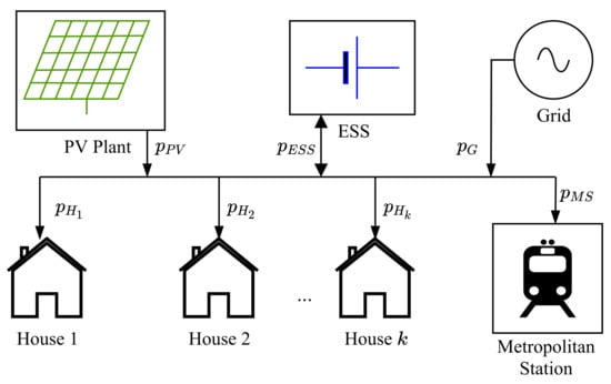
Figure 1.
Power system architecture.
The subsystems of this architecture can be classified in two categories: loads and power sources. In this case, the loads are presented by the houses of the district and the metropolitan station . The power supplies are the PV plant and the Grid. We consider the Grid as a power supply, thus excluding the case where we can inject surplus energy. The reason for considering this hypothesis is related to the fact that future energy communities do not focus on injecting energy into the grid, relying more on collective self-consumption.
Moreover, it is important to mention that the ESS can be included in both categories, depending on the operational mode (if the battery is discharging, then the ESS acts as a power source, and it acts as a load if the battery is charging ). Thus, the architecture represents a first representation of the subject investigated in the paper, which focuses on the question of how to optimally exploit the flexibility provided by the ESS in order to minimise the interactions with the Grid.
Thus, from a power system perspective, we can establish an energy balance for the system in Equation (4).
The importance of this balance equation in the modeling process is twofold: Firstly, this equation acts as a constraint and must be satisfied at every moment during the simulation scenario; secondly, it establishes a signing convention between the power exchanges inside the system. Furthermore, it is imperative to note that the power variables used in the simulations represent hourly average values for each respective power system, including PV power.
These aspects will be further emphasised in the following subsections, where we describe the modeling approach and data processing for each subsystem.
4.2. District Model
In order to model the district energy consumption, we consider the load profiles of 91 houses, along with the load profile of a metropolitan station.
The houses’ load profiles have been determined by measuring the consumption from the main appliances in each home. For the work presented in this paper, the selected time horizon was one day, with a sample rate of one hour. The consumption data was obtained from the IRISE database as part of the REMODECE project [29], where multiple residential houses in several geographical areas have been monitored.
The metropolitan station investigated in this case study represents an urban underground subway station, part of the Bucharest (Romania) subway network. The station is subject to intense passenger daily traffic, correlated with high level power consumption. In this manner, we aim to investigate a scenario in which the subway station power system acts as a significant load for the district, thus being a suitable solution to increase the overall self-consumption of the community during peak production periods. The load profile of the subway station has been obtained by a dedicated measuring project implemented by the subway network company of Bucharest (Romania).
In order to develop the metropolitan station power model, we consider a typical subway station architecture, which is depicted in Figure 2. The architecture is designed according to typical metropolitan stations built in Bucharest, Romania [30].
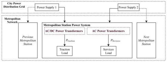
Figure 2.
Typical metropolitan station power system structure.
As it can be observed, the architecture depicts an automatic supply switch mechanism that allows stations to have reserve supply power in the case of faulty behaviour or malfunctions. However, by analysing the power flow inside the station, a clear separation from the rolling stock powering system and the auxiliary services power system can be observed. While the first subsystem is responsible for powering the trains, the second subsystem is responsible for powering all the other loads that may exist in a metropolitan station: ventilation systems, lighting systems and so on.
Thus, we can consider a simplified model of the total load in a metropolitan station to be the following:
where represents the total load of a subway station, represents the rolling stock load and represents the energy consumed by the auxiliary systems in the station.
Consequently, at district level, the total power consumption can be defined as follows:
where represents the power of each house indexed by j.
In this scenario, the district power consumption represents a particular case given the utility scale consumer (the subway station) combined with the other residential loads. Figure 3 emphasizes the differences between the respective power profiles.
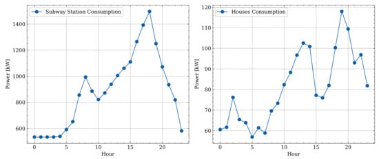
Figure 3.
Power profile comparison between the the subway station and district houses.
As it can be observed, the residential power profile emphasizes increased consumption in the afternoon and evening that is related to increased activity by the residents after returning home from work.
On the other hand, the subway station power profile is characterised by two consumption peaks, specifically around 8 a.m. and 6 p.m. These peaks are correlated to passenger traffic during commuting times, since the rolling stock consumes much more energy when it is full.
Nevertheless, the magnitude difference between the two profiles can be clearly noticed, with the subway station consuming significantly more energy then the residential part of the district (even during the night, during maintenance works when rolling stock activity is halted).
4.3. PV Plant Model
The power produced by the PV plant can be obtained by measuring solar irradiation at the respective location and by applying the following model [31]:
where represent the power produced by the PV plant, represents the power rating of a module, n represents the number of PV modules, represents a correction factor to consider power losses through the inverter, temperature variations and wire transmissions, G represents the incident solar irradiance and represents the irradiance at standard temperature conditions (1 kW/m). To take into account possible power losses and other uncertainties (such as those presented in [32] for other renewable energy sources), we only consider the correction factor in a PV power model that can be easily used in linear optimisation problems due to its simplicity. Moreover, it is important to note that this type of model can be used in various configurations with different module types due to the explicit description of PV power as a product between the number of panels and nominal power rating of a PV module.
4.4. Energy Storage System Model
In order to develop the energy storage system model, we have to consider the dynamic flow of power that can occur inside the battery: power proceeding from the battery to the system during the discharge process and power arriving inside the battery during the charge process. To quantify the current state of the battery at a precise moment t, we considered the battery State of Charge (SOC). More precisely, the SOC represents the amount of the nominal capacity of the battery (kWh) that is available for usage in the system as (kWh).
In the research presented in this paper, in order to depict the dynamics of SOC during the simulations, we considered a simplified type of an Energy Reservoir Model [33]. As such, according to the sign convention established, the change of SOC with respect to a time interval can be expressed as follows:
where represent the power moving in or out from the storage system. It is important to note here that respects the sign convention established by the power balance Equation (4). Thus, if the battery is charging, then , and if the battery is discharging, .
Consequently, the discrete form of the ESS model that has been used in the simulations can be analysed in Equation (10):
where represents the SOC at step i, and represents the sample rate. As it was mentioned in the previous section, the sample rate for the entire district is chosen at 1 h.
4.5. Optimisation Problem Formulation
Considering the models described in the previous section, an optimisation problem is formulated in order to size the PV plant and ESS and also to optimally control the respective storage system.
The problem formulation can be analysed from two perspectives: a sizing optimisation perspective in which we aim to determine what would be the optimal size for the respective subsystems mentioned before and a control perspective for the energy storage system. This is an important aspect since, by formulating only a typical sizing problem, the formulation will not include the impact of the battery. The idea is to take into account both the optimal trajectory of the battery and the optimal size of the system, thus providing a global solution. In the applied context, after the PV plant is designed, the optimal trajectory will be imposed in daily operational mode.
Consequently, the following part will address the control perspective at first and then emphasize the necessary elements to formulate the optimisation problem as a sizing problem as well.
As stated in other specialised literature reviews [33], the scope is to formulate the optimal control problem in the following general manner:
where x represents the decision variable vector, is the objective that must be minimised through the control action, represents a vector of equality constraints enforced upon the control variable and represents a vector of inequality constraints. The optimal control action is determined for a specific horizon of time .
In the presented work, as mentioned in the previous sections, the objective is to optimally control the ESS in order to minimise the NEEG. Thus, the objective becomes the following:
where represents the total load of the district, and m is the number of hours of . and are known data sets for production and consumption, respectively, while represents a set of real variables that is part of decision vector x.
Considering both the optimisation objective (Equation (12)) and the causality of the battery model (Equation (10)), we can understand the optimal control problem as an optimal scheduling problem where we know the initial ESS SOC. More specifically, for the battery optimisation horizon , we may have a multitude of possible routes for to follow from the initial point, as described by Figure 4.
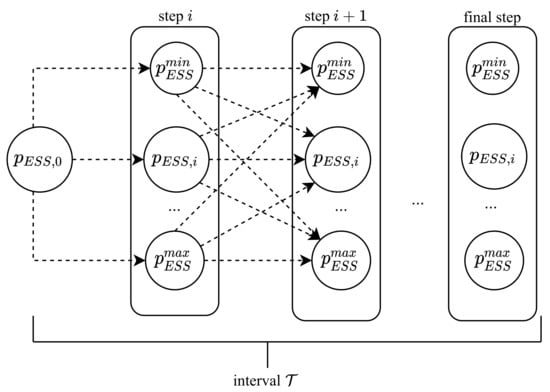
Figure 4.
Battery control as an optimal schedule problem.
By taking into account the sizing problem as well, the objective of the optimal control problem is to determine the optimal solution x:
where m is the size of the time horizon , is a real variable representing the size of the ESS and n is an integer variable representing the number of PV modules.
Equation (12) represents the adapted form that also takes into account the impact of battery in the overall Microgrid operation as a discrete model for the control horizon . It can be observed that the signing convention established by the balance (Equation (4)) is also taken intro account, as can be either a power source if the ESS is discharging (thus, having a positive value) or a load if the ESS is charging (thus, having a negative value). In this manner, the flexibility offered by the battery is mathematically expressed in relation to the NEEG.
However, we aim to formulate a linear programming optimisation problem; thus, we want to express Equation (12) in linear form. Thus, using the respective transformation for absolute value [34], the objective to minimise collective NEEG (Equation (12)) becomes the following:
where e is a newly introduced continuous variable.
It is important to know the fact that the decision vector x is dependent in size relative to the length of the time horizon ; thus, the complexity of the problem may grow significantly if we consider longer periods of time.
In order to properly address this limitation, we may formulate the optimisation problem for a short period of time (i.e., a day) and impose a constraint to allow us to use the strategy in a cyclic manner, one day at a time. This constraint can be expressed in terms of SOC for the optimisation horizon as follows.
To write this constraint in linear form depending on our decision variables, we must determine the expression of with respect to . Therefore, we can use the model of the ESS (Equation (10)) to obtain the following.
Thus, only if the following is the case:
which represents the linear form of constraint in Equation (15), expressed in terms of the decision variable.
Thus, if we elaborate upon the situation in which the optimisation horizon is a day, the initial SOC must be equal to the final SOC in order to apply the strategy for the next day when the final SOC from the day before becomes the initial SOC in the current day.
Since the decision vector is set, constraints have been considered in order to properly adapt the model for the presented context. First, the SOC must be limited between two values in order to preserve the battery life. Thus, we have the following.
In order to implement this constraint in linear form, we must write this constraint for each . Based on Equation (16), we have two constraints:
where j is used as an index to iterate through all SOCs until hour i. , and all represent continuous variables. thus, the final linear constraint becomes the following.
Furthermore, the charge and discharge power must be limited between certain thresholds in order to operate in safe conditions. We can express this constraint in terms of SOC relative to a an imposed limit that is available as a measure for both the discharge and charge operations. Considering the signing convention we set a priori, the constraint may be expressed as the following.
In this case, we must also express the constraint in terms of in a linear form. For any , we can write the following.
Thus, the set of linear constraints for the charge and discharge power becomes the following.
On another hand, there may be situations in which the ESS may be charged from the Grid; however, this would affect the battery life by increasing the number of charge–discharge cycles. Thus, to preserve the battery life, we must consider storing only the energy that is produced by the PV plant; in other words, we have the following:
Finally, in order to determine the optimal sizing of the PV plant and battery, we consider the number of PV panels n and the battery nominal capacity to be decision variables and, therefore, are included in the decision vector x. However, we must also limit the sizes up to certain thresholds. This may be expressed as the following.
In the simulation scenarios further presented, the optimisation problem has been used in the Mixed Integer Linear Programming (MILP) form and has been resolved using the Coin-or Branch and Cut (CBC) solver.
5. Results and Discussion
The optimisation problem has been resolved using a Mixed Integer Linear Approach for a time interval of one day. Several simulations cases have been developed in order to assess the impact of the most important parameters over the SC and SS. As it was mentioned before, even though the collective NEEG is used as an objective in the optimisation problem, it is more meaningful to analyse the results through the evaluation of the collective SC and SS.
The optimisation problem is resolved in each scenario for one day (). Thus, considering Equations (13), (20), (23) and (25), the implemented optimisation problem has a decision vector x of 25 variables, with 168 inequality constraints, 24 equality constraints and 4 bounding constraints.
Therefore, three simulation scenarios are investigated: a scenario in which we investigate the impact of choosing over SS and SC; a scenario in which we investigate the impact of ; and a scenario in which we investigate the choice of the initial SOC. In each scenario, the power rating of chosen PV modules is 500 W, with a correction factor . The ESS nominal voltage is 400 V.
5.1. Impact of on the Collective SC and SS
Figure 5 illustrates the power flow in the system for three investigated cases in which the is set a priori at either 1200 kWh, 1600 kWh or 2000 kWh before resolving the optimisation problem.
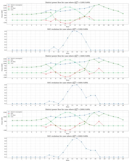
Figure 5.
Comparison between results of optimisation with different ESS capacity limits. Case 1: = 1200 kWh; Case 2: = 1600 kWh; Case 3: = 2000 kWh.
For all simulation scenarios, configuration parameters are presented in Table 1, Table 2 and Table 3.

Table 1.
Configuration for the first simulation scenario.
Table 2.
Configuration for the second simulation scenario.
Table 3.
Configuration for the third simulation scenario.
Moreover, the obtained solution can be investigated in Table 4. For all the simulation scenarios implemented, the results for collective SC and SS with storage (identified in the table as and ) are compared with the values obtained for SS and SC with the same PV configuration n but without ESS.
Table 4.
Results comparison.
By analysing the SS and SC indexes with and without ESS, it can be observed that, as expected, the ESS provides an important increase in SC and a moderate increase in SS. Thus, it is clear that the newly included flexibility in terms of storage provides a certain economical benefit because the SS also acts a reduction in energy bill. More specifically, if we have a SS index equal to 0.3, then the energy bill will be 30% lower. Moreover, in terms of SC, the ESS is able to maximise the SC to the upper limit, thus allowing the district to fully benefit from the produced renewable energy.
However, since the flexibility provided by the ESS improves both SC and SS, the algorithm always provides a configuration with the highest capacity possible. Even if a SC value equal to one is achieved for a capacity of 1600 kWh, further simulation with higher capacities provided further moderate increases in the SS index. This aspect can be addressed by adequately choosing the for the problem or by introducing other criteria, such as initial ESS investment, etc.
On another hand, if the ESS capacity is too small, the benefit in terms of SS and economic impact may be too small to be considered, and quantities of energy may be wasted due to the impossibility of injecting it into the grid.
5.2. Impact of on Colective SC and SS
Thus, after the first simulation scenario, we analyse the impact of different charge–discharge limits constraining the optimal ESS control. In this case, it is known that charging or discharging the ESS too fast has an important impact on battery life; thus, a charge–discharge constraint must be introduced.
The simulation results for this scenario can be analysed in Figure 6.
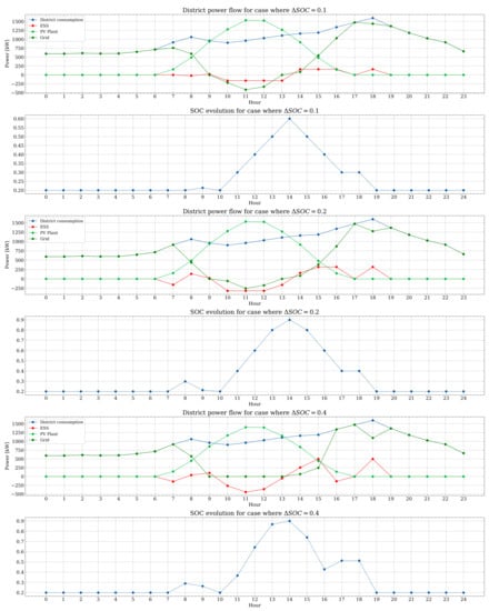
Figure 6.
Comparison between results for optimisation with different charge/discharge limit. Case 1: ; Case 2: ; Case 3: .
Results are presented in Table 4 by using a comparison between system without ESS and system with ESS.
As it can be observed, by comparing to the first simulation scenario, choosing a charge–discharge limit that is too small significantly impacts the SC and SS indexes. The reason is that the battery does not have enough time during the PV production period to charge to the maximum allowed , thus resulting in a decrease in flexibility. However, an increase in charge–discharge limit also results in performance increase, but as it was mentioned beforehand, battery life must always be considered.
5.3. Impact of on the Collective SC and SS
Another simulation scenario is related to the choice of the initial SOC. The objective is to understand if the choice of the initial SOC impacts the SC and SS of the system over the day.
In this scenario, three cases where considered, where . The results can be analysed in Figure 7, and the numerical results are in Table 4. The configuration used in this scenario is presented in Table 3.
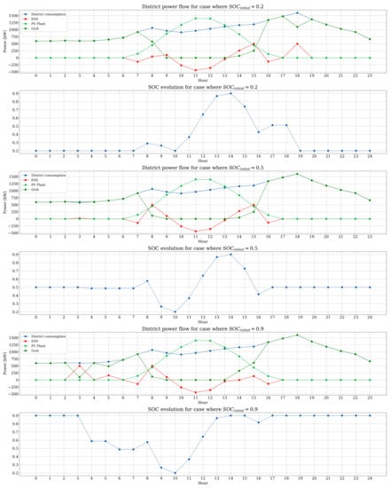
Figure 7.
Comparison between results with different initial SOC. Case 1: ; Case 2: ; Case 3: .
In this scenario, it can be observed that the SS and SC indexes are the same, regardless the initial SOC. This is related to the nature of the load and the PV production period. More specifically, due to the fact that the district load is relatively high throughout the day, with two consumption peaks during the morning and the evening, the only aspect influenced by the initial SOC is the time of discharging. We can observe that if the initial SOC is 0.2, then the ESS is discharging in the afternoon. On the other hand, if the initial SOC is 0.9, according to the optimal control, the ESS is discharging during the morning. If the initial SOC is 0.5, then the discharging process is divided between mornings and afternoons with respect to the charging process during the PV production period.
Consequently, the initial SOC choice may adjusted according to different energy cost regulations in countries. For example, there may be periods where the energy from the grid is cheaper; thus, the initial SOC might be adjusted in this manner.
6. Conclusions
The paper considers a method of involving people in energy management of a district, in a scenario with a large urban consumer (a metropolitan station) and an ESS that provides power flexibility to the system. The aim of the research study is to try and use the shared renewable energy sources of the district, along with the flexibility provided by the storage and the large consumption requirements of a metropolitan station, in order to capitalize the benefit obtained from collective self-consumption and collective self-sufficiency.
In this direction, the paper uses the presented optimisation strategies as instruments to control the available power flexibility in order to satisfy the community consumption needs using PV energy, while aiming to maximise the collective self-consumption and self-sufficiency at the district level. More specifically, the proposed concept is used to determine the optimal trajectory of the ESS power over the day in order to minimise the net energy exchanged with the grid. The formulation can also be used to determine the optimal size of the PV plant and the ESS, with the same objective as mentioned before.
The main contribution of this paper is related to optimisation problem formulation in a sharing context (at district level) that includes two components, an optimal sizing component and an optimal control component, which further address the objective of minimising the net energy exchanged with the grid, thus maximising the collective self-consumption and self-sufficiency of the community. Moreover, the results are investigated for a district of houses that includes a subway station, which is a utility scale urban consumer. Comparing to other relevant recent works, the paper address both the optimal sizing and optimal control issues of an ESS at the district level, aiming to provide solutions related to the novel collective self-consumption and collective self-sufficiency objectives. Moreover, instead of providing a multi-objective approach that would rather prove to be difficult in terms of weight choosing, the proposed solution provides a simple single-objective MILP problem, thus paving the path for obtaining a global optimal solution.
The results obtained in the simulations indicated that the optimal control of the ESS provides increased flexibility to the collective self-consumption and self-sufficiency of the district. In most simulations, the self-consumption of the system was very close to the absolute maximum value, stating that almost all produced energy is used internally. On another hand, an increase in collective self-sufficiency was noted, indicating a smaller community energy bill and also an indirect form of economical profit. As it can be observed in Table 4, in comparison with the scenario without storage, the SS may increase up to 4% with ESS, providing an energy bill that is reduced at almost 36% (since SS is equivalent to the energy bill reduction and ). Moreover, SC may reach the peak value of one, showing an increase up to 14% compared to the case without storage. Thus, all the produced PV energy can be consumed internally in the community.
Future investigations will also address other forms of energy-related flexibility, such as electrical vehicles or by modifying the load and possibly asking citizens to shift consumption during specific periods of the day. A limitation of the presented work is related to the nature of the flexibility provided by the ESS. Thus, in future research, by also considering citizen involvement and electric vehicles, this limitation might be addressed, and the performances of the community might also be better.
The concept of collective self-consumption, albeit a recent one, is already introduced in many countries regulations; thus, much more research is needed to properly provide reliable solutions in terms of energy management strategies.
Author Contributions
Investigation, M.S.S.; Conceptualization, I.F.; writing—review and editing, M.S.S., I.F. and S.P.; Software, V.C.; Validation, V.C., S.P.; Supervision, I.F., S.P.; All authors have read and agreed to the published version of the manuscript.
Funding
This research received no external funding.
Institutional Review Board Statement
Not applicable.
Informed Consent Statement
Not applicable.
Acknowledgments
The authors would like to thank the Romanian subway network company METROREX S.A. for the data used in presented research.
Conflicts of Interest
The authors declare no conflict of interest.
Abbreviations
The following abbreviations are used in this manuscript:
| PV | Photovoltaic; |
| ESS | Energy storage system; |
| SC | Self-consumption; |
| SS | Self-sufficiency; |
| NEEG | Net energy exchanged with the grid (Wh); |
| Continuous representation of collective self-consumption; | |
| Continuous representation of collective self-sufficiency; | |
| Discrete representation of collective self-consumption; | |
| Discrete representation of collective self-suficiency; | |
| Energy produced by PV (Wh); | |
| Consumption of a system (Wh); | |
| Charge/discharge energy for a system (Wh); | |
| Time interval; | |
| Sampling time (h); | |
| m | Number of samples in time interval ; |
| Power produced at sample i (W); | |
| Power produced at sample i (W); | |
| Charge/discharge power for ESS at sample i (W); | |
| Power consumed by house j (W); | |
| k | Number of houses; |
| Power from the grid (W); | |
| Power consumed by the metropolitan station (W); | |
| Power consumed by the trains passing in the metropolitan station (W); | |
| Power consumed by auxiliary services in the metropolitan station (W); | |
| n | Number of PV modules; |
| Nominal power of a PV module (W); | |
| G | Solar irradiance; |
| Irradiance at standard temperature conditions; | |
| SOC | ESS state of charge; |
| Nominal capacity of ESS (kWh); | |
| Available capacity of ESS (kWh); | |
| Limit capacity of ESS (kWh); | |
| Inferior limit to (W); | |
| Superior limit to | |
| SOC at the beginning of simulation; | |
| SOC at the end of simulation; | |
| Inferior limit to ; | |
| Inferior limit to ; | |
| Charge discharge limit; | |
| Limit to number of PV modules. |
References
- Frieden, D.; Roberts, J.; Gubina, A.F. Overview of emerging regulatory frameworks on collective self-consumption and energy communities in Europe. In Proceedings of the International Conference on the European Energy Market, EEM, Ljubljana, Slovenia, 18–20 September 2019. [Google Scholar] [CrossRef]
- European Parliament and Council of the European Union. Directive (EU) 2018/2001 of the European Parliament and of the Council of 11 December 2018 on the promotion of the use of energy from renewable sources. Off. J. Eur. Union 2018, 11–22. [Google Scholar]
- European Parliament and Council of the European Union. Directive 2019/944 on Common Rules for the Internal Market for Electricity. Off. J. Eur. Union 2019, 16. [Google Scholar]
- Tan, K.M.; Babu, T.S.; Ramachandaramurthy, V.K.; Kasinathan, P.; Solanki, S.G.; Raveendran, S.K. Empowering smart grid: A comprehensive review of energy storage technology and application with renewable energy integration. J. Energy Storage 2021, 39, 102591. [Google Scholar] [CrossRef]
- Azevedo, J.A.; Santos, F.E. A More Efficient Technique to Power Home Monitoring Systems Using Controlled Battery Charging. Energies 2021, 14, 3846. [Google Scholar] [CrossRef]
- Dargahi, A.; Ploix, S.; Soroudi, A.; Wurtz, F. Optimal household energy management using V2H flexibilities. Int. J. Comput. Math. Electr. Electron. Eng. 2014, 33, 777–792. [Google Scholar] [CrossRef]
- Van der Meer, D.; Wang, G.C.; Munkhammar, J. An alternative optimal strategy for stochastic model predictive control of a residential battery energy management system with solar photovoltaic. Appl. Energy 2021, 283, 116289. [Google Scholar] [CrossRef]
- Sortomme, E.; El-Sharkawi, M.A. Optimal power flow for a system of microgrids with controllable loads and battery storage. In Proceedings of the 2009 IEEE/PES Power Systems Conference and Exposition, PSCE 2009, Seattle, WA, USA, 15–18 March 2009; pp. 1–5. [Google Scholar] [CrossRef]
- Hosseini, S.M.; Carli, R.; Dotoli, M. A residential demand-side management strategy under nonlinear pricing based on robust model predictive control. In Proceedings of the Conference Proceedings—IEEE International Conference on Systems, Man and Cybernetics, Bari, Italy, 6–9 October 2019; pp. 3243–3248. [Google Scholar] [CrossRef]
- Merei, G.; Moshövel, J.; Magnor, D.; Sauer, D.U. Optimization of self-consumption and techno-economic analysis of PV-battery systems in commercial applications. Appl. Energy 2016, 168, 171–178. [Google Scholar] [CrossRef]
- Dongol, D.; Feldmann, T.; Schmidt, M.; Bollin, E. A model predictive control based peak shaving application of battery for a household with photovoltaic system in a rural distribution grid. Sustain. Energy Grids Netw. 2018, 7. [Google Scholar] [CrossRef]
- Cao, M.; Xu, Q.; Qin, X.; Cai, J. Battery energy storage sizing based on a model predictive control strategy with operational constraints to smooth the wind power. Int. J. Electr. Power Energy Syst. 2020, 115, 105471. [Google Scholar] [CrossRef]
- Maheshwari, A.; Paterakis, N.G.; Santarelli, M.; Gibescu, M. Optimizing the operation of energy storage using a non-linear lithium-ion battery degradation model. Appl. Energy 2020, 261, 114360. [Google Scholar] [CrossRef]
- Engels, J.; Claessens, B.; Deconinck, G. Techno-economic analysis and optimal control of battery storage for frequency control services, applied to the German market. Appl. Energy 2019, 242, 1036–1049. [Google Scholar] [CrossRef] [Green Version]
- Kolcun, M. Electrical Energy Flow Algorithm for Household, Street and Battery Charging in Smart Street Development. Energies 2021, 14, 3771. [Google Scholar] [CrossRef]
- Rae, C.; Bradley, F. Energy autonomy in sustainable communities—A review of key issues. Renew. Sustain. Energy Rev. 2012, 16, 6497–6506. [Google Scholar] [CrossRef]
- McKenna, R.; Merkel, E.; Fichtner, W. Energy autonomy in residential buildings: A techno-economic model-based analysis of the scale effects. Appl. Energy 2017, 189, 800–815. [Google Scholar] [CrossRef] [Green Version]
- Casals, M.; Gangolells, M.; Forcada, N.; Macarulla, M.; Giretti, A. A breakdown of energy consumption in an underground station. Energy Build. 2014, 78, 89–97. [Google Scholar] [CrossRef] [Green Version]
- Fanti, M.P.; Mangini, A.M.; Roccotelli, M.; Ukovich, W. District Microgrid Management Integrated with Renewable Energy Sources, Energy Storage Systems and Electric Vehicles. IFAC-PapersOnLine 2017, 50, 10015–10020. [Google Scholar] [CrossRef]
- Sameti, M.; Haghighat, F. Integration of distributed energy storage into net-zero energy district systems: Optimum design and operation. Energy 2018, 153, 575–591. [Google Scholar] [CrossRef]
- González-Gil, A.; Palacin, R.; Batty, P.; Powell, J.P. A systems approach to reduce urban rail energy consumption. Energy Convers. Manag. 2014, 80, 509–524. [Google Scholar] [CrossRef] [Green Version]
- Faranda, R.; Leva, S. Energetic sustainable development of railway stations. In Proceedings of the 2007 IEEE Power Engineering Society General Meeting, PES, Tampa, FL, USA, 24–28 June 2007; pp. 1–6. [Google Scholar] [CrossRef]
- Stefan Simoiu, M.; Calofir, V.; Fagarasan, I.; Arghira, N.; Stelian Iliescu, S. Towards Hybrid Microgrid Modelling and Control. A Case Study: Subway Station. In Proceedings of the 24th International Conference on System Theory, Control and Computing, ICSTCC 2020—Proceedings, Sinaia, Romania, 8–10 October 2020; pp. 602–607. [Google Scholar] [CrossRef]
- Siad, S.; Damm, G.; Galai Dol, L.; De Bernardinis, A. Design and control of a DC grid for railway stations. In Proceedings of the PCIM Europe 2017—International Exhibition and Conference for Power Electronics. Intelligent Motion, Renewable Energy and Energy Management, Nuremberg, Germany, 16–18 May 2017. [Google Scholar] [CrossRef]
- Perez, F.; Iovine, A.; Damm, G.; Galai-Dol, L.; Ribeiro, P. Regenerative Braking Control for Trains in a DC MicroGrid Using Dynamic Feedback Linearization Techniques. IFAC-PapersOnLine 2019, 52, 401–406. [Google Scholar] [CrossRef]
- Cano, A.; Arévalo, P.; Benavides, D.; Jurado, F. Sustainable tramway, techno-economic analysis and environmental effects in an urban public transport. A comparative study. Sustain. Energy Grids Netw. 2021, 26, 100462. [Google Scholar] [CrossRef]
- Roberts, M.B.; Bruce, A.; MacGill, I. A comparison of arrangements for increasing self-consumption and maximising the value of distributed photovoltaics on apartment buildings. Sol. Energy 2019, 193, 372–386. [Google Scholar] [CrossRef]
- Jiménez-Castillo, G.; Muñoz-Rodriguez, F.J.; Rus-Casas, C.; Talavera, D.L. A new approach based on economic profitability to sizing the photovoltaic generator in self-consumption systems without storage. Renew. Energy 2020, 148, 1017–1033. [Google Scholar] [CrossRef]
- REMODECE Project. Available online: https://remodece.isr.uc.pt (accessed on 5 August 2021).
- Simoiu, M.S.; Stamatescu, G.; Calofir, V.; Fagarasan, I.; Iliescu, S.S. Comparative Analysis of Predictive Models for Subway Rolling Stock Energy Forecasting. In Proceedings of the 23rd Conference On Control Systems And Computer Science, Bucharest, Romania, 26–28 May 2021. [Google Scholar]
- HOMER. PV Power Estimation. Available online: https://www.homerenergy.com/products/pro/docs/latest/how_homer_calculates_the_pv_array_power_output.html (accessed on 10 December 2020).
- Scarabaggio, P.; Grammatico, S.; Carli, R.; Dotoli, M. Distributed Demand Side Management with Stochastic Wind Power Forecasting. IEEE Trans. Control. Syst. Technol. 2021, 1–5. [Google Scholar] [CrossRef]
- Rosewater, D.M.; Copp, D.A.; Nguyen, T.A.; Byrne, R.H.; Santoso, S. Battery Energy Storage Models for Optimal Control. IEEE Access 2019, 7, 178357–178391. [Google Scholar] [CrossRef]
- Matoušek, J.; Gärtner, B. Understanding and Using Linear Programming; Springer: Berlin/Heidelberg, Germany, 2007; pp. 11–20. [Google Scholar] [CrossRef] [Green Version]
Publisher’s Note: MDPI stays neutral with regard to jurisdictional claims in published maps and institutional affiliations. |
© 2021 by the authors. Licensee MDPI, Basel, Switzerland. This article is an open access article distributed under the terms and conditions of the Creative Commons Attribution (CC BY) license (https://creativecommons.org/licenses/by/4.0/).