Abstract
The reference characteristics of complex permittivity of the transformers insulation solid component were determined for use in the precise diagnostics of the power transformers insulation state. The solid component is a composite of cellulose, insulating oil and water nanoparticles. Measurements were made in the frequency range from 10−4 Hz to 5000 Hz at temperatures from 293.15 to 333.15 K. Uncertainty of temperature measurements was less than ±0.01 K. Pressboard impregnated with insulating oil with a water content of (5.0 ± 0.2) by weight moistened in a manner maximally similar to the moistening process in power transformers was investigated. It was found that there are two stages of changes in permittivity and imaginary permittivity components, occurring for low and high frequency. As the temperature increases, the frequency dependencies of the permittivity and imaginary permittivity component shifts to the higher frequency region. This phenomenon is related to the change of relaxation time with the increase in temperature. The values of relaxation time activation energies of the permittivity ΔWτε′ ≈ (0.827 ± 0.0094) eV and the imaginary permittivity component ΔWτε″ = 0.883 eV were determined. It was found that Cole-Cole charts for the first stage are asymmetric and similar to those described by the Dawidson–Cole relaxation. For stage two, the charts are arc-shaped, corresponding to the Cole-Cole relaxation. It has been established that in the moistened pressboard impregnated with insulating oil, there is an additional polarization mechanism associated with the occurrence of water in the form of nanodrops and the tunneling of electrons between them.
1. Introduction
For many years, insulation of power transformer windings has been made from cellulose (in the form of paper and pressboard) and mineral oil. Currently, synthetic aramid paper [1,2,3,4,5] has been introduced in the production of transformer parts. As a liquid component of the insulation, synthetic and natural esters are used in some transformers [6,7]. The transformers currently working in power systems are dominated by those with paper-oil insulation. In paper insulation, aging phenomena occur during operation. Namely, there is the so-called depolymerization of cellulose fibers, which results in a reduction in fiber length. This results in the reduction of mechanical parameters of material and the occurrence of a small amount of water molecules in them [8,9]. Often times more moisture gets into the transformer from the outside. Then the moisture is dissolved in oil, which supplies it to the cellulose. The solubility of water in cellulose is several decades higher than in oil [10]. Therefore, the moisture is absorbed by the cellulose, where its content gradually increases over time. The moisture content of the cellulose during the long-term operation of transformers gradually increases from an initial level of about 0.7–0.8% by weight to as much as 5% by weight and more. This is a limit value, exceeding which can lead to a catastrophic failure of the transformer [11,12,13]. As a result of the failure, transformer oil leaks out and ignites. The effects of this are very harmful to the environment because mineral oil is poorly biodegradable [14,15,16]. The burning of transformer oil causes a large amount of toxic smoke [17,18,19,20]. In order to prevent a breakdown, the moisture content of the cellulose must be checked. Chemical methods for the determination of water content in cellulose are known [21]. However, due to the fact that the power transformer is made as a hermetic construction, a cellulose sample cannot be taken for testing. Therefore, non-destructive methods are used to determine the moisture content. These are primarily electrical methods whose application requires the determination of so-called reference characteristics. These are the dependencies of electrical parameters determined in a laboratory for a moistened pressboard. The estimation of insulation moisture levels is based on a comparison of transformer insulation electrical parameter measurements results and reference characteristics, simultaneously taking into account geometrical dimensions of transformer solid insulation and oil channels.
Considering the type of voltage used in measurements, the electrical methods used for transformer diagnostics can be divided into two groups. The group of DC methods includes Return Voltage Measurement (RVM) [22,23,24] and Polarization Depolarization Current (PDC) [25,26,27]. The Frequency Domain Spectroscopy (FDS) method [28,29,30] uses alternating voltage in the low and ultra-low frequency ranges. Currently, meters dedicated to testing electrical transformers are manufactured. These meters can perform measurements using RVM, PDC, FDS methods and their combinations [31,32,33]. Currently, FDS meters are widely used to diagnose the condition of solid insulation in terms of moisture. FDS meters return the real C′ and imaginary C″ components of the composite complex capacity calculated on the basis of their own software. Using the C′ and C″ values and the geometric dimensions of the insulation, it is possible to calculate the material parameters to which the article is devoted:
where ε′—relative dielectric permittivity (real component), ε″—imaginary part of permittivity (imaginary component), d—thickness of dielectric, S—surface area of flat capacitor electrode, C′—real component of capacity, C″—imaginary component of capacity.
The FDS meter software allows for the cellulose insulation moisture level estimation. Recently, there has been a report [33] that the moisture values determined with the measuring software differ from the actual values determined by chemical methods. Underestimation of moisture level, determined by FDS meters, may result in a delay in deciding what action to take to prevent transformer failure. Underestimation of moisture level using FDS meters can be caused by the two following factors. The first is the traditional way of preparing reference samples for testing. For this purpose, the pressboard is vacuum dried and then humidified in atmospheric air, where the moisture is absorbed by a dry pressboard. After moisturization, the reference sample is impregnated with transformer oil at the atmospheric pressure [34,35,36,37,38,39,40,41]. The process of pressboard moisturization in power transformers is different. After vacuum drying, the transformer is filled with oil under vacuum. During many years of operation, the moisture level of oil-impregnated cellulose gradually increases by water absorption from the oil.
The failure of the FDS method in the determination of cellulose moisture, especially in older transformers [42] may also be caused by the use of simplified models of relaxation processes in analysis and the occurrence of strong temperature dependencies of the parameters measured. The basis for the analysis of FDS results is a number of dielectric relaxation models. The first of them is the Debye model [43]. It assumes that the polarization is caused by the orientation of water molecules in the electric field. The model assumes that all dipoles have the same relaxation time τ0. The Cole-Cole relaxation model [44,45] assumes that the relaxation time τ0 is the expected value of the probability function of relaxation time distribution. There are also other relaxation models, for example, the Davidson–Cole empirical model [46,47]. The distribution containing the most empirical parameters was proposed by Havriliak and Nagami [48].
The formula describing the above models include dielectric permittivity ε′ and imaginary permittivity component ε″, which are components of the complex permittivity:
where ε*—complex permittivity of composite, ε′—real permittivity component, ε″—imaginary permittivity component, j—imaginary unit.
From the models presented [43,44,45,46,47,48] above, it follows that when the frequency is lowered to zero (to DC voltage), the conductivity also decreases to zero. This means that the resistivity of the material should increase infinitely. This is contrary to all the experimental results known so far, which in the ultra-low frequency range shows a certain limit of conductivity, equal to DC conductivity. In the paper [49], it was experimentally established that in the ultra-low frequency region, the AC conductivity exactly equals the DC conductivity of moistened oil-impregnated insulating pressboard.
In papers [50,51], on the basis of studies on the dependence of DC conductivity on the moisture content in the insulating oil-impregnated pressboard, it has been established that the conduction takes place through electron tunneling between water molecules. Constant and alternating current studies, on the other hand, have shown that water in moist pressboard impregnated with insulating oil [51,52] occurs in the form of nanodrops with diameters of about 2.2 nm, containing about 200 water molecules each. Tunneling of the electron from one electrically neutral nanodrop causes it to obtain a positive charge. Simultaneously, the closest nanodrop to which the electron has tunneled obtains a negative charge. In this way, by tunneling, dipoles in the form of near nanodrops of water are formed. Such a dipole has a dipole torque, many times greater than that of water molecules. This is due to the fact that the distance between the nanodrops is many times greater than the distance between positive and negative charges in the water molecules.
The formation of such large dipoles causes additional polarization of the material [53,54]. Due to the structure of energy states, the tunneling electron requires additional thermal energy. Such polarization, due to the influence of thermal energy, is called additional thermally activated polarization. After some time, the electron from a negatively charged well tunnels back into the positive well and thus the dipole disappears. In the case of polarization caused by electron tunneling, the relaxation time τ is an important parameter of the phenomena. It is the time from the moment the dipole is formed after the electron jumps from one electrically neutral potential well to another, until the moment the electron returns to the well from which it started its jump. The value of relaxation time has a significant influence on the value of permittivity caused by the hopping electron exchange as well as on the frequency range in which it occurs. Relaxation time is a function of the distance between the nanodrops to which the electron tunnels, high-frequency dielectric permittivity of the medium in which the nanodrops are located, and temperature [52].
For the transformer insulation condition diagnosis, including the cellulose insulation moisture level estimation, the FDS method is currently the most commonly used. Measurements using the FDS method were performed both in laboratory conditions and on transformers, usually three points per decade, to shorten the measurement time [29,55,56,57].
The aim of this study was to determine the reference frequency–temperature dependences of permittivity and imaginary permittivity components of pressboard, moistened in a manner as similar as possible to the process of cellulose moistening in power transformers. Diagnostics on the basis of reference dependencies make it possible to determine states threatening transformer failure and thus to avoid environmental pollution. A pressboard with a water content limit value of (5.0 ± 0.2) by weight, exceeding which threatens transformer failure and environmental pollution with poorly biodegradable transformer oil, was investigated. Precise measurements of permittivity and imaginary permittivity components of the composite of cellulose, transformer oil and water nanoparticles were performed, with the number of measurement points per decade several times higher than in the previous tests, in the temperature range 293.15–333.15 K with a step of 8 K. For the tests, a climate chamber was used. The uncertainty of temperature maintenance and measuring was less than ±0.01 K during many hours of testing. For the analysis of the obtained results, the model of alternating and direct current hopping conductivity was used, which was developed on the basis of the quantum mechanical electron tunneling phenomenon. The results of the direct and alternating current conductivity tests of the composite of cellulose, insulating liquid and water nanoparticles perfectly agree with this model [49,52,58,59,60,61].
2. Materials and Methods
Thus far, samples of a moistened and oil-impregnated pressboard used for determining the reference characteristics have been prepared as follows. The pressboard was dried for up to about 72 h in a vacuum chamber at a temperature of about 353 K. After drying using the Karl Fischer Titration method [21], residual water content was determined. Then the mass, which should be obtained by the sample after moistening it to the set value, was determined, taking into account the residual water content. The sample was left in the air in order to absorb moisture from the atmosphere. At the same time, the mass of the pressboard was constantly controlled until the calculated value, i.e., the assumed moisture level, was reached. After reaching the calculated mass, the sample was put into transformer oil or other insulating liquid for impregnation [29,34,56,58]. Such a method of moistening is very far from the process of cellulose moistening in power transformers. In transformers, the cellulose is dried and then impregnated in vacuum conditions. During many years of operation, the moisture penetrates into the transformer and dissolves in oil. Then the oil delivers it to dry impregnated cellulose insulation. Cellulose absorbs moisture from oil because the solubility of moisture in the cellulose is several decades higher than in oil [10]. As a result, the natural process of cellulose moistening in a transformer differs significantly from the way samples are prepared for laboratory tests. Therefore, the use of standard dependencies obtained on samples prepared in the previous way may cause a discrepancy with the values obtained for transformers.
To produce the samples tested in this work, a method of moistening was used, as close as possible to the natural moistening of pressboard in transformers [49]. The process of sample preparation was carried out in the following way. Two plates of the pressboard were vacuum-dried, moistened in atmospheric air and immersed in insulating oil for impregnation. These plates served as a source of moisture for the third one. The third sample was vacuum-dried and impregnated with oil in the vacuum. Then the dry vacuum impregnated sample was placed between two previously moistened plates, located in a vessel with oil. In order to eliminate contact, the plates were separated with brackets. The plate to be tested was moistened in the same way as pressboard moistening in power transformers. Namely, moisture from previously moistened plates diffused into the oil. The oil transferred the moisture to the impregnated dry sample, where it was absorbed by cellulose. The moistening time of the sample to be tested was over a year and a half.
The measurements presented in this paper were carried out on a plate prepared in a manner as close as possible to natural moistening in a transformer. The tests were performed on a plate with water content of (5.0 ± 0.2)% by weight, as accumulation of water above this value may lead to failure. The materials used in the study were Weidman’s electrotechnical pressboard and Nynas’ transformer oil with a moisture content of several ppm, prepared by a specialist company for filling of a power transformer after the renovation. Both insulating materials are dedicated for building insulation of power transformers. Wetting, drying and impregnation were carried out on 1 mm thick slabs of pressboard, shown in Figure 1. Then samples were cut from the slabs to be tested. Their diameters were 160 mm. A view of the test sample before wetting is shown in Figure 1a and after drying, wetting and impregnation with insulating oil in Figure 1b.
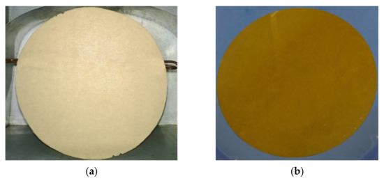
Figure 1.
View of the test sample before moistening (a) and after moistening, drying and impregnation with insulating oil (b).
Measurements were made in a three-electrode measuring system. The measuring station was presented and described in References [58,62]. The measuring system with the tested sample was placed in a hermetic vessel, flooded with a small amount of oil. The oil level was above the pressboard plate. Then the measuring system and the plate were placed in a climate chamber.
Figure 2 shows a photograph of the test station used in this paper to measure the AC parameters of a composite of electrical pressboard—insulating oil—water nanodroplets [63]. The climate chamber used in the research has been equipped with an electronic control system—proportional-integral-differential controller (PID), forced air circulation and chilled air source. To achieve and stabilize the set temperature of the measuring capacitor, due to its mass, a time of approx. 15 h is needed. After reaching the preset temperature, the climate chamber maintains it for many hours. The measuring system temperature is controlled by a PT 1000 sensor and AGILENT 34970A temperature meter (Agilent Technologies, Santa Clara, CA, USA) and recorded in the computer memory every 1 s. The uncertainty of measurement and temperature stabilization type A, determined on the basis of 108,000 measurement points, is less than ±0.01 K [62].
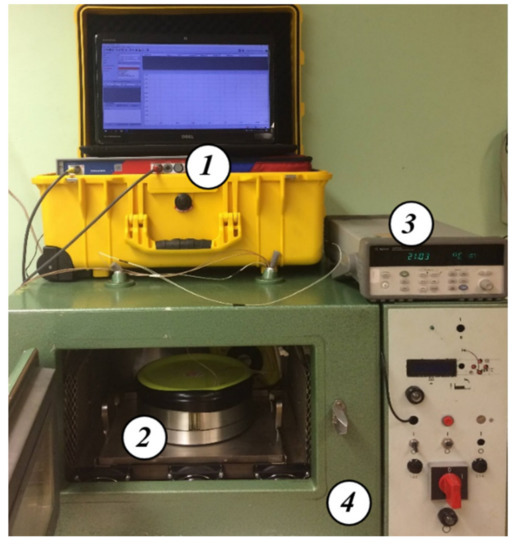
Figure 2.
Photograph of the test stand for alternating current measurements of electrical properties of liquid–solid insulations [63]: 1—DS-PDC Dielectric Response Analyzer (Dirana meter), 2—three-electrode capacitor, 3—Agilent temperature meter, 4—climatic chamber.
As is well known, measurements of the values of the real and imaginary components of the combined permittivity can only be made using an alternating current forcing. The measurements were made with the Dirana meter—FDS-PDC dielectric response analyzer (OMICRON Energy Solutions GmbH, Berlin, Germany) manufactured by Omicron. The measuring frequency range of the meter is from 0.0001 to 5000 Hz at a voltage of up to 200 V. In many cases, laboratory measurements using the FDS method are performed at three points per decade [34,64]. In a similar way, as a rule, tests of energy transformers are also performed [29,65]. This is due to the very high time-consuming character of measurements in the ultra-low frequency area, of the order of 0.001 Hz and lower.
Alternating current measurements in the study were performed in the frequency range from 10−3 to 5000 Hz at 10 points per decade. In the range from 10−4 to 10−3 Hz, 6 points per decade were recorded. This improved the accuracy of the reference characteristics determination. Further improvement of the reference characteristics accuracy determination was achieved by increasing the number of measurement temperatures and decreasing the temperature measurement and maintenance uncertainty. Measurements were performed at 6 measurement temperatures 293.15, 301.15, 309.15, 317.15, 325.1 and 333.15 K. A computer program was developed to control the operation of the meters and climate chamber and to collect the measurement results. It allows for remote control of the stand.
3. Results and Discussion
3.1. Frequency–Temperature Relationships of Dielectric Permittivity
Figure 3 shows in the form of points the results of the alternating current permittivity measurements of the composite of cellulose, synthetic ester and water nanoparticles for its content of (5.0 ± 0.2)% by weight measured at temperatures from 293.15 to 333.15 K with step 8 K. We will analyze its frequency dependence on the example of a measurement for 333.15 K.
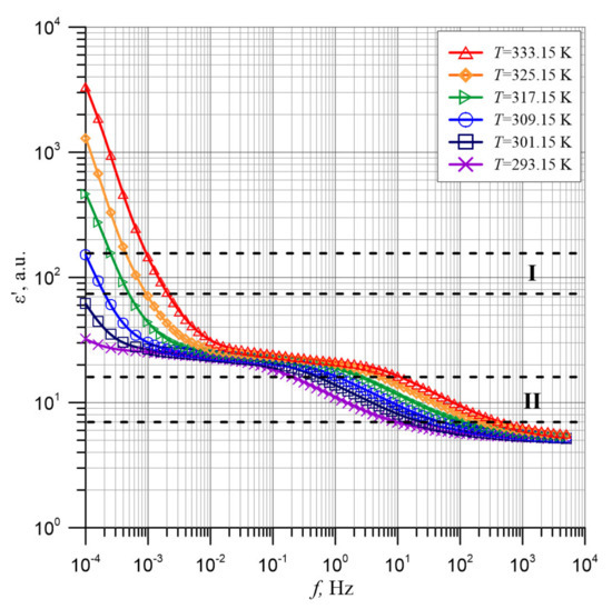
Figure 3.
Frequency dependence of permittivity of the composite of cellulose, transformer oil and water nanoparticles for its content of (5.0 ± 0.2)% by weight measured at temperatures from 293.15 to 333.15 K. Continuous lines—polynomial approximation.
In the ultra-low frequency area, the permittivity values are very high. Thus, for a frequency of 10−4 Hz at 333.15 K, its value is above 3000. An increase in frequency causes the permittivity to drop to a value below 30 with further stabilization at this level. In the frequency area above 1 Hz, the permittivity is further reduced to a value of about five with further stabilization at this level. This means that there are two stages of polarization changes in the composite, low and high-frequency one. From Figure 3, it follows that in both areas of permittivity values stabilization, permittivity is practically not dependent on temperature. This means that the determined permittivity value at the end of the first (low-frequency) stage is its high-frequency permittivity ε′∞1. The same value is the static permittivity ε′S2 for the second stage. At the end of the second stage the value of the high-frequency permittivity ε′∞2, is determined. As shown in Figure 3, for the high-frequency stage, both static and high-frequency permittivity values were determined. For the low-frequency stage only the high-frequency permittivity was determined. It is likely that static permittivity for this stage can be achieved at frequencies below the Dirana frequency range of 10−4 Hz.
We will now analyze the effect of temperature on the frequency relationships of the permittivity. Figure 3 shows that as the temperature rises, the curves move to a higher frequency area. This is due to the change in relaxation time as the temperature rises. In studies [50,52] it has been established that the transfer of charges, determining the conductivity and polarity of the moist pressboard impregnated with insulating oil, takes place through electron tunneling between nanodrops of water. In Reference [52], a relaxation time formula for electron tunneling between water nanodrops was derived:
where τ0L—numerical coefficient, r—average distance between the potential wells between which the electron tunnels, R0—radius of location of the wave function of the jumping electron (Bohr radius), β—numerical coefficient, the value of which is β ≈ (1.75 ± 0.05) [66], ΔW0—activation energy of the conductivity, k—Boltzman constant, U—dipole potential energy.
In Formula (4), U is the potential energy of a dipole, formed after electron tunneling from one electrically neutral nanodrop of water to another, i.e., the closest one. Its value is given by the formula:
where e—electron charge, ε0—dielectric permittivity of vacuum, ε′∞m—high-frequency permittivity of dielectric matrix, r—distance between adjacent nanodrops of water.
Due to the fact that a sample with moisture content of (5.0 ± 0.2)% by weight was tested, the distance r between nanodrops remains unchanged while changing temperature. Therefore, a generalized activation energy value ΔW can be entered in Formula (4):
where and .
In order to precisely calculate the temperature dependence of the relaxation time described by Formula (6), permittivity values between adjacent measuring points will be needed. In order to determine these values, a polynomial approximation of the experimental values was made, which was performed using the method proposed in the paper [56]. As Figure 3 shows, the experimental permittivity values are within a wide range of several decades. They are a function of frequency, which changes in the area of eight decades. In order to limit the range of such large changes of parameters approximated, the approximation for logarithms of these values was applied [67]. In order to eliminate errors that arise during approximation at the beginning and at the end of the approximation range, extrapolation of data points outside the measuring ranges was applied. Extrapolations were performed both in the area of lower and higher frequencies. The results of such polynomial approximation are shown in Figure 3 as solid lines. Each of these lines consists of 200 points per decade, calculated from the formula for polynomial approximation. High quality of approximation is proved by the values of determination coefficients R2 for different measurement temperatures presented in Table 1. Table 1 shows that the lowest of the obtained R2 = 0.999936 value is very close to unity.

Table 1.
R2 values for the approximation of polynomial permittivity for different measurement temperatures.
The high quality of experimental results approximation is also confirmed by the percentage differences between the approximation waveforms and the experimental results shown in Figure 4. Higher values of the differences are found in the ultra-low frequency area. The greatest of the differences, occurring for the two frequency values, do not exceed 1.4%. The remaining differences are smaller and decrease with frequency increase. In the frequency range above 10−1 Hz, the differences are 0.1% and smaller. These results are highly satisfactory.
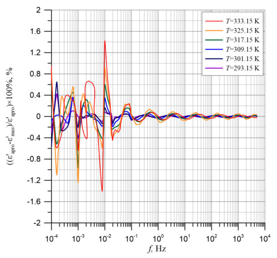
Figure 4.
Permittivity differences between the permittivity test results for the composite of cellulose, transformer oil and water nanoparticles for temperatures from 293.15 to 333.15 K and calculated polynomial approximation.
Figure 5 shows the values of derivatives, calculated according the formula d(logε′)/d(logf) on the basis of approximations. The figure shows that the transition from the low-frequency permittivity dependence to the high-frequency dependence is separated by a section with very small derivative values of about 0.02–0.03. The very small values of derivative in this frequency area are due to the small impact of the permittivity from the first stage, for which the permittivity tends to achieve a steady state of ε′∞1 = ε′S2. This means that in these frequency ranges, the low-frequency permittivity for stage 2 reaches the constant value ε′S2 = const.
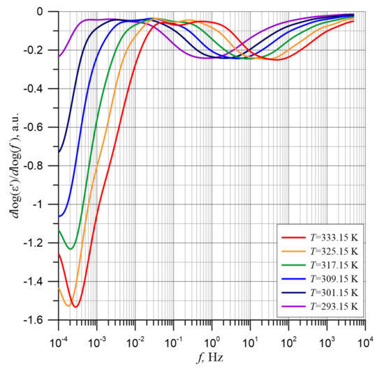
Figure 5.
Frequency dependence of d(logε′)/d(logf) derivatives for temperatures from 293.15 to 333.15 K.
In Figure 5, two distinct minima can be observed, which correspond to the points of the quickest permittivity drop. The first minimum determines the rate of permittivity change in the low-frequency stage. It is located in the ultra-low frequency area and is only visible for temperature of 317.15 K and above. For lower temperatures, the minimum is located at frequencies below the lower limit of the Dirana meter. The second minimum moves as the temperature increases into the higher frequency area. The shift as the temperature increases both in the permittivity waveforms (Figure 3) and in the derivatives minima (Figure 5) means that the relaxation times for both stages decrease as the temperature increases.
In order to determine the activation energy of relaxation time value, determined by Formula (6), two ranges (I and II), marked with horizontal dashed lines, in which rapid changes in permittivity are observed, have been selected on the temperature relationships of the permittivity (Figure 3). In the area between these ranges, as shown in Figure 5, changes are hardly visible. Formula (6) will be simplified by starting from the following assumptions. Relaxation time, with an accuracy of a non-specified value of the constant A can be written in the form:
where εi′—our chosen permittivity value from ranges I or II in Figure 3, the same for all measurement temperatures, A—a more or less undefined constant value, fi(T)—the frequencies at which ε′i occurs for different temperatures.
Taking into account Formulas (6) and (7), we can write it down in the form:
Since the experimental results give the permittivity relationship ε′i as a function of frequency, we will transform Formula (8) into a form suitable to determine the activation energy of relaxation time:
The factor before the exponent in Formula (9) contains constant values. This allows the Arrhenius chart to be drawn. Figure 6 shows Arrhenius charts for 5 permittivity values in the I (low-frequency) range, and for 10 values in the II (high-frequency) range.
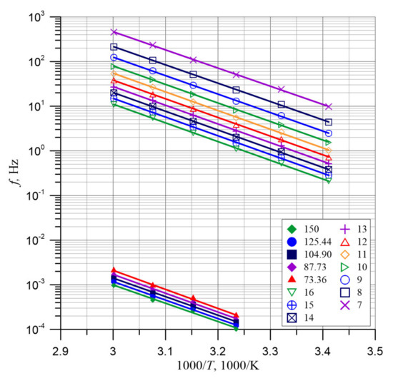
Figure 6.
Arrhenius diagrams for determination of the permittivity activation energy of relaxation time.
In Figure 6, straight lines show the linear approximation of the data points, obtained by the method of smallest squares. The coefficients of determination R2 for curves from Figure 6 are shown in Table 2. The smallest value of R2 is 0.99612 and is very close to unity. This means the high quality of linear approximation and high accuracy of permittivity and temperature measurements. As Figure 6 shows, the curves for all permittivity values are placed practically parallel. This means that the activation energies for the different permittivity values are similar. The activation energies of the relaxation times for the different permittivity values determined from the approximation formulae for the 15 curves from Figure 6 are shown in Table 2.
Table 2.
Activation energies for the relaxation time of electrical permittivity and determination factors R2 for the runs shown in Figure 6.
The data presented in Table 2 show that the mean value of the activation energies of the permittivity relaxation time, determined on the basis of 15 values, is equal to ΔWτε′ ≈ (0.827 ± 0.0094) eV. The application of 15 permittivity values from I and II ranges allowed to obtain a very low uncertainty of activation energy determination, which is only 0.0094 eV or 1.14%. Figure 7 shows the dependence of the individual activation energy of relaxation time of the permittivity values on the permittivity value, the mean value and the mean value ± uncertainty of its determination. Figure 7 shows that the activation energies of the permittivity relaxation times for both the first and the second stage are equal within the uncertainty limits.
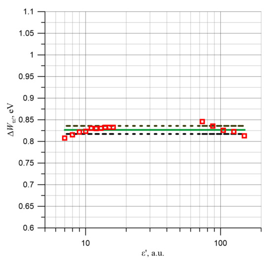
Figure 7.
Relaxation time activation energy values ε′ determined for 15 permittivity values from Figure 3, mean value and mean value ± uncertainty of determination.
Using this fact, the mean activation energy of relaxation time of the permittivity has been converted from 301.15 K and above to an electrical engineering reference temperature of 293.15 K. The results of conversion are presented in Figure 8.
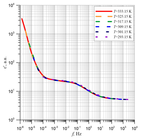
Figure 8.
Permittivity relationships ε′ for different measurement temperatures converted to a reference temperature of 293.15 K by means of the average activation energy of the relaxation time value.
As shown in Figure 8, after shifting with use of the activation energy of relaxation time, all six curves obtained at different measurement temperatures overlap perfectly. This means that the shape of the pressboard and mineral oil composite frequency dependences of permittivity are determined by the content of water nanoparticles. The position of the permittivity curves in relation to the frequency axis depends on temperature through the activation energy of relaxation time, described by Formula (6). As is well known, measurements on real power transformers are made at various insulation temperatures—usually not coinciding with the temperatures used in laboratory measurements. Establishing that the waveform obtained at any temperature can be converted to the reference temperature by means of the activation energy of relaxation time of the permittivity means that the measurements results made on real power transformers can be converted to the reference temperature of 293.15 K. This will allow for determination of the cellulose insulation moisture content after taking into account the geometrical dimensions of the solid insulation and the oil channels. This will enable accurate diagnostics of the insulation and thus detection of conditions threatening the failure and hence environment contamination.
3.2. Frequency–Temperature Imaginary Part of Permittivity Dependence
Figure 9 shows the experimental frequency dependences of the ε″ imaginary part of permittivity for temperatures from 293.15 to 333.15 K. The values of imaginary permittivity component ε″ were calculated from the values of the imaginary capacity C″ given by Dirana meter and the surface area of the measuring electrode S and the thickness of pressboard d using Formula (2). Figure 9 shows that in the ultra-low frequency area, a very fast decrease in the imaginary permittivity component value is observed. In the area from about 10−2 to about 1 Hz, depending on the temperature, the rate of reduction slows down. It then increases slightly and reaches a local maximum. Then the next area of the imaginary permittivity component decrease is observed.
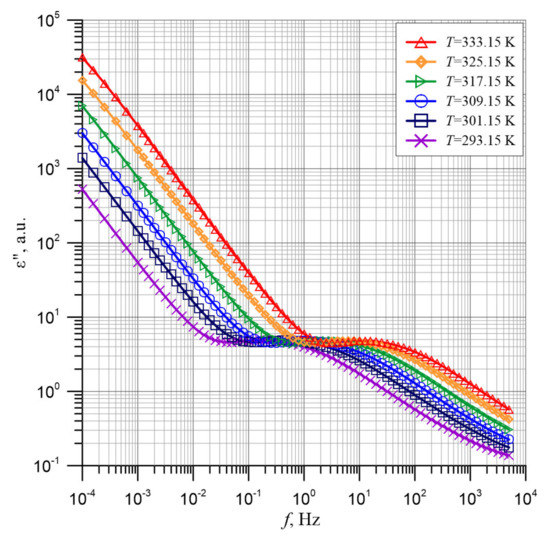
Figure 9.
Frequency dependence of imaginary permittivity component of the composite of pressboard, mineral oil and water nanoparticles for temperatures from 293.15 to 333.15 K. Points—experimental results, continuous lines—approximation results.
As Figure 9 shows, the test points are relatively densely spaced. However, for further analysis, points in between will be needed. In order to obtain the intermediate points, as in the case of permittivity described above, polynomial approximation of the experimental results was performed using the method proposed in Reference [67]. The approximation results are presented in Figure 9 as solid lines, each of which consists of 200 points per decade.
The differences between experimental results and polynomial approximation results, presented in Figure 10, show the high quality of the approximation results performed using the method proposed in Reference [67]. The figure shows that the biggest difference occurs near the frequency of 10−2 Hz and its value is about 0.5%. In the remaining frequency ranges, the differences are even smaller.
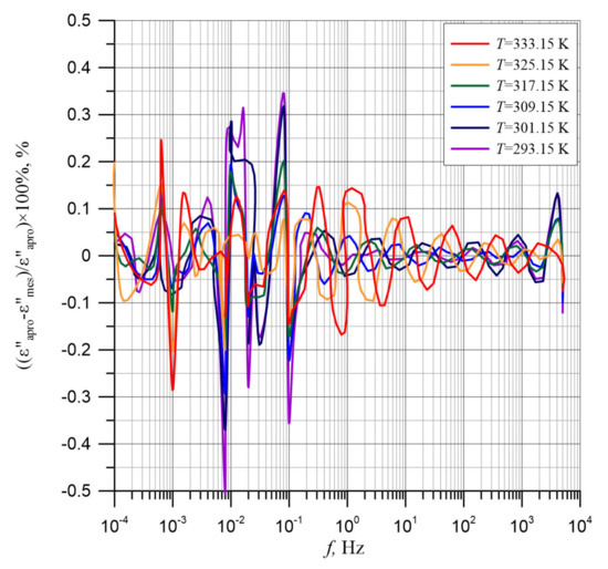
Figure 10.
Percentage differences between the experimental imaginary permittivity component results for the composite of cellulose, transformer oil and water nanoparticles for temperatures from 293.15 to 333.15 K and polynomial approximation results.
As we know, the imaginary part of permittivity ε″ is determined by the formula [43,48]:
where σ—conductivity, ω—angular frequency, ε0—vacuum permittivity.
Formula (10) includes the conductivity σ, which is a function of temperature, ω and ε0, the values of which do not depend on temperature. As established in [49], the position of σ curves in the double logarithmic coordinates is affected simultaneously by the temperature dependence of conductivity and the temperature dependence of the relaxation time of conductivity. Both these factors are determined by the same activation energy, the mean value of which equals ∆Wστ ≈ (0.894 ± 0.0134) eV [49]. Formula (10) shows that the activation energies of the imaginary permittivity component value and its relaxation time are identical to the corresponding activation energies for conductivity.
As we know [43], the frequency at which the maximum imaginary permittivity component value occurs is related to the expected value of the imaginary permittivity component relaxation time by the formula:
where fmax—frequency where maximum imaginary permittivity component occurs, τ0—expected value of relaxation time.
Determining the relaxation time from the local maximum position on the relation ε″(f) from Formula (11) allows to determine its real value. In order to determine the exact position of the maximum ε″(f) for the different measurement temperatures, the values of derivatives from formula d(logε″)/d(logf) are determined. The results of the calculations based on polynomial approximation are shown in Figure 11.
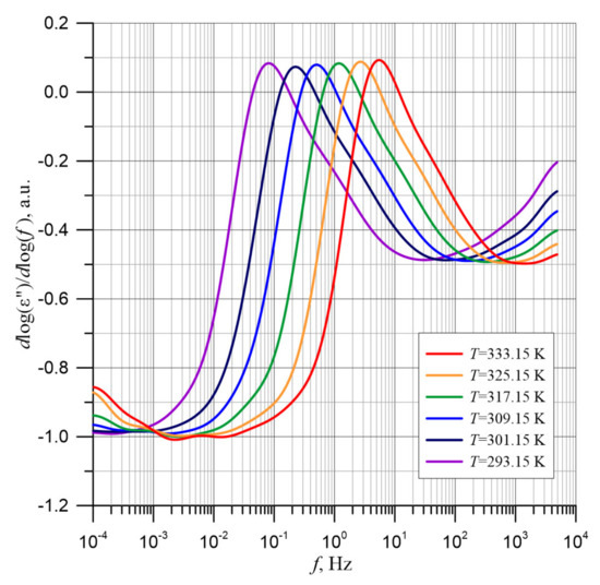
Figure 11.
Frequency dependence of the derivative d(logε″)/d(logf) for the composite of pressboard, mineral oil and water nanoparticles for temperatures from 293.15 to 333.15 K.
As we know, at the function extremes, the value of the derivative is equal to zero. The maximum position is represented by a change in the derivation value from positive to negative with an increase in the value of the argument. On this basis, the frequencies at which the maxima occur for all measurement temperatures were determined from Figure 11. Then, from Formula (11), the expected values of the relaxation times were calculated, and for them, the Arrhenius diagram, shown in Figure 12, was developed.
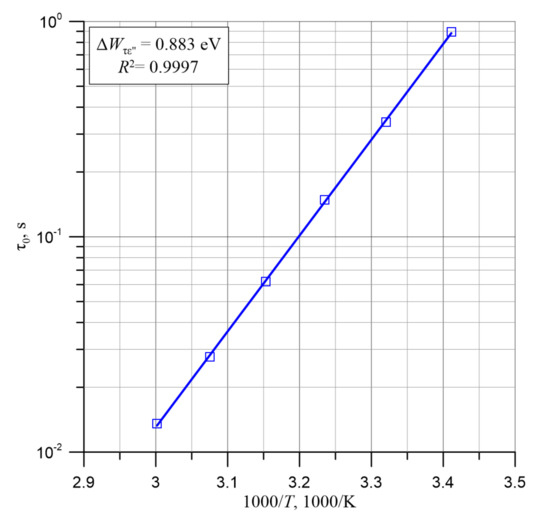
Figure 12.
Arrhenius diagram for the values of expected relaxation time, determined from the position of the imaginary permittivity component frequency dependence maximum and its linear approximation.
The approximation curve, determined by the least squares method, is a linear relationship. The determination factor R2 = 0.9997 is close to unity. It proves a high accuracy of approximation. Calculated from the approximation formula, as shown in Figure 13, the value of the activation energy of relaxation time of the imaginary permittivity component is ΔWτε″ = 0.883 eV. This value is equal, within the limits of uncertainty, to the mean values obtained in [49] for the activation energy of the relaxation time of the conductivity ∆Wστ ≈ (0.894 ± 0.0134) eV. The difference is only 0.011 eV or 1.2%.
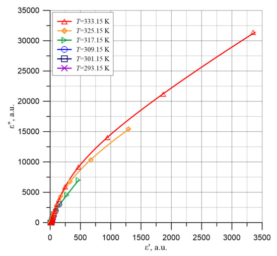
Figure 13.
Cole-Cole diagrams in the area of high permittivity ε′ for the composite of cellulose, transformer oil and water nanoparticles for temperatures from 293.15 to 333.15 K.
3.3. Analysis of the Cole-Cole Diagrams of Imaginary Part of Permittivity as a Function of Permittivity
The Dirana meter returns real C′ and imaginary C″ capacity values. On their basis, using the geometric dimensions of the tested sample, the permittivity ε′ and imaginary permittivity component ε″ are calculated, which are the components of the complex dielectric permittivity ε* of the composite. These values are described by Equations (1)–(3). The frequency relationships ε′(f) and ε″(f) are determined by the dielectric relaxation mechanism. A number of different dielectric relaxation processes can occur in insulation materials. The best known are the Debye, Cole-Cole and Davidson–Cole distributions [43,44,45,46,47].
In the cases of Debye and Cole-Cole type dielectric relaxation, combined permittivity is described by a formula:
where ε*—complex permittivity, εs—low-frequency permittivity (static), ε∞—high-frequency permittivity, j—imaginary unit, ω—angular frequency, τ0—expected value of relaxation time, α—numerical factor.
The value α = 0, corresponds to Debye’s relaxation mechanism. The Debye relaxation mechanism assumes that all dipoles in a dielectric material have the same relaxation time value τ0 = const. Values 0 < α < 1 occur in the Cole-Cole relaxation mechanism. In this mechanism, a probability distribution of relaxation times occurs, and τ0 is the expected value of relaxation time.
For the analysis of dielectric relaxation phenomena, the dependence of imaginary permittivity component ε″ on the permittivity value ε′ is used:
Dependency (13) is shown in the Cole-Cole chart. In the case of Debye’s relaxation, relation (13) takes the shape of half a circle in the chart. For the Cole-Cole relaxation, it takes the form of an arc. In some materials, a Davidson–Cole distribution [46,47] take place, described by the formula:
where β < 1.
The physical justification of this distribution is not as easy as in the cases of the Debye and Cole-Cole distributions and is mainly empirical. The graphs described by distribution (14) are asymmetric. In the low ε′ area, the increase in ε″ values is slower than in the circle. In the higher ε′ area, the ε″ decrease is close to the circle. The distribution containing the most empirical parameters was proposed by Havriliak and Nagami [48]. Apart from the four above-mentioned relaxation distributions, there are a number of others. As shown in paper [68], the shape of ε″ = f(ε′) graphs is related to the relaxation mechanism found in insulation material. This article lists seven possible mechanisms, and the corresponding seven different shapes of the relation ε″ = f(ε′) curves. Each of these mechanisms occurs in a different range of measuring frequencies, starting from ultra-high EHF through high HF, medium MF, low LF, very low VLF to ultra-low ELF. In our case, the use of the low to ultra-low frequency range eliminates four of the seven relaxation mechanisms listed in this article.
In Figure 13, Cole-Cole dependencies are presented, for which ε′ values from Figure 3 and ε″ from Figure 9 have been used. The figure shows that ε″ = f(ε′) dependencies may be similar to those described by the Davidson–Cole empirical relaxation. It does not seem possible to analyze the waveforms presented in Figure 13 more closely. This is due to the fact that these waveforms are still very far from reaching the maximum, behind which a decrease in ε″ should be observed.
From Figure 13, it follows that in the area of the lowest ε′ values there are some peculiarities. In order to explain them, Figure 14 shows the waveforms ε″ = f(ε′) for low values of the ε′ argument.
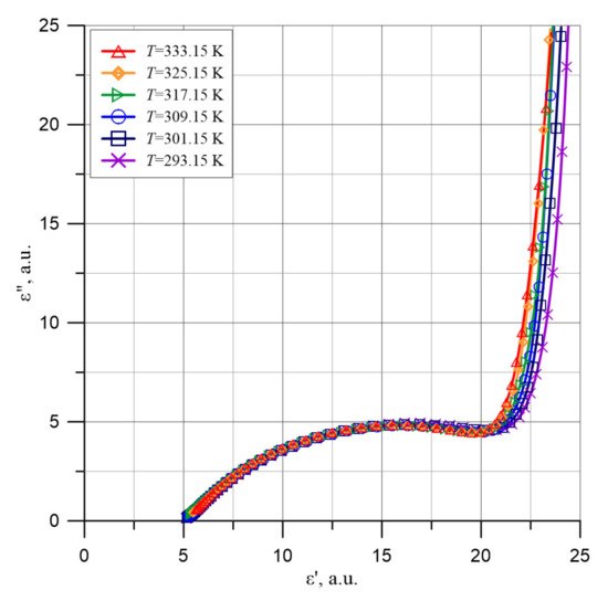
Figure 14.
Cole-Cole charts in the low permittivity area ε′ for the composite of cellulose, transformer oil and water nanoparticles based on experimental data for temperatures from 293.15 to 333.15 K.
Figure 14 shows that in the area of permittivity ε′ from about 5 to about 19, the shape of the waveform is similar to the curve described by the Cole-Cole relaxation, Formula (12) at α < 1.
In order to determine the center position of the circle, the values of derivatives d(ε″)/d(ε′), presented in Figure 15, were determined. The values presented in Figure 15 were calculated on the basis of the graphs obtained by polynomial approximation of ε′ and ε″ (Figure 3 and Figure 9). As is known, the derivative is a tangent line to the dependency curve. The normal to the circle tangent line is the line on which the center of the circle lies. In order to determine the center of the circle, two tangent lines to different points on the circle were chosen and normal lines to them were determined. The center of the circle lies at the intersection of the normal lines to the tangents.
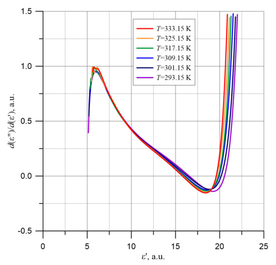
Figure 15.
Values of d(ε″)/d(ε′) derivatives in the low permittivity area ε′ for the composite of cellulose, transformer oil and water nanoparticles based on approximation results for temperatures from 293.15 to 333.15 K.
The formula for the normal to tangent at the point with the coordinates [εp′, εp′] lying on the circle is given by:
where x, y—coordinates of points on the tangent line, xp, yp—coordinates of a point on the circle the tangent passes through, fꞌ(xp)—value of the derivative to the circle at that point.
Formula (15) is fair to all xp, except the xp for which f′(xp) = 0.
At the point of intersection of the two normals to the tangent, the values of the coordinates are the same. This point is the center of the circle. Therefore, at this point, the x0 and y0 coordinates of the normal points must be equal:
By transforming Formula (16), the formula is obtained for x0—the coordinate of the center of the circle:
In order to determine the value of y0, we substitute the obtained value x0 in of Equation (16). After obtaining the coordinates of the center of the circle, we calculated the radius of the circle:
By substituting the values of coordinates and derivatives for the two points on the arc shown in Figure 14 with Formulas (16)–(18), the radius r = 14.4 and coordinates of the center of the circle ε′ = 15.9, ε″ = −9.6 are determined. Figure 16 shows the plot of the circle, the coordinates of its center and its radius, calculated from Formulas (16)–(18).
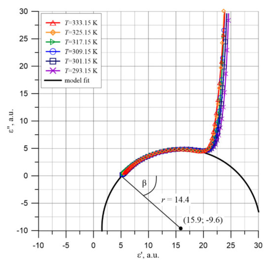
Figure 16.
Cole-Cole diagrams in the low permittivity area ε′ for the composite of cellulose, transformer oil and water nanoparticles and the circle describing the relation ε″ = f(ε′).
For the Cole-Cole relaxation, the angle β (Figure 16) between the ε′ axis and the radius of the circle at ε∞, expressed in radians, is related to the value α entered in Formula (12) [45]:
By substituting the numerical values for Formula (21), we obtain a value of α = 0.658.
Using the obtained α value of the Cole-Cole distribution for a composite of pressboard, mineral oil and water nanodrops with a moisture content (5.0 ± 0.2)% by weight, we can write the equation:
We will now analyze the polarization mechanism occurring at the second high-frequency stage of permittivity changes. As is known, the dielectric permittivity of capillary-free and pore-free cellulose is ε′∞c = 6.6 [69]. In the pressboard used in the work, there are capillaries, the volume of which is about (15–20)% of the sample volume. The capillaries are filled with insulating oil of permittivity ε′∞o = 2.3 [70]. This results in a decrease in the resultant permittivity of an oil-impregnated pressboard. This means that the value ε′∞2 = 5.2 obtained in work is the high-frequency permittivity of an oil-impregnated pressboard. As Figure 16 shows, the circle of the Cole-Cole diagram intersects the x-axis at points ε∞2 = 5.2 and εS2 = 26.6. This means that the moisture content of the cellulose results in an increase in permittivity at stage 2 from about 5.2 to about 26.6, i.e., by 21.4. In some publications, for example, in [55], the increase in permittivity is attributed to the polarization of water molecules. The static permittivity of water at 293.15 K is known to be about ε′w = 80 [71]. It follows that if the increase in pressboard permittivity of the second stage by about 21.4 is due to the polarization of the water, its content in the pressboard is about 27% by weight. The moisture content of the pressboard tested was (5.0 ± 0.2)% by weight and was over five times lower. A number of other parameters characterizing water polarization do not agree with these assumptions. The relaxation time of water molecules at room temperature is about 10−11 s [72]. From our measurements, the value of relaxation time in the second stage at room temperature is only 0.8 s (Figure 12). The second stage of permittivity occurs at frequencies f ≤ 104 Hz (Figure 3). The static permittivity of water at temperatures above 273.15 K occurs up to a frequency of about 109 Hz [72]. The comparison of polarization characteristics obtained in the study at stage 2 and relevant parameters concerning water polarization shows unequivocally that water in an oil-impregnated pressboard is not in the state of a liquid with macroscopic volumes. This means that in a moistened pressboard impregnated with insulating oil, there is an additional mechanism of polarization, causing more than a fivefold increase in permittivity compared to the value caused by water alone in the form of a liquid. Additional polarization is related to the presence of water in the form of nanodrops. Tunneling of electrons from one electrically neutral nanodrop to another causes the formation of dipoles with dipole moments many times greater than the dipole moment of water molecules. This is manifested by an additional polarization of the composite.
4. Conclusions
In this paper, reference characteristics of permittivity and imaginary permittivity components of cellulose—insulating oil—water nanoparticle composites were determined. They form the basis for accurate diagnosis of the transformer insulation state. Diagnostics made on the basis of reference relations makes it possible to determine the states threatening transformer failure and thus to avoid environmental pollution. The tests were carried out for a pressboard with a water content of (5.0 ± 0.2) by weight.
In the frequency range from 10−3 to 5000 Hz, measurements were made with a resolution of 10 points per decade, in the range 10−4 to 10−3 Hz, and six points per decade were recorded. Measurements were made for measurement temperatures 293.15, 301.15, 309.15, 317.15, 325.15 and 333.15 K. The uncertainty of temperature maintenance and measurement was less than ±0.01 K.
It was observed that in the ultra-low frequency area, the permittivity values are very high. Thus, at a frequency of 10−4 Hz at a temperature of 333.15 K, its value is above 3000. An increase in frequency causes a decrease in permittivity to below 30 with further stabilization at this level. In the frequency area above 1 Hz, there is a further decrease in permittivity to about a value of five with a transition to the steady state. This means that there are two stages of polarization changes in the composite, at low and high-frequency.
As the temperature increases, the frequency dependencies of the permittivity shifts into the higher frequency area. This is related to the reduction of the relaxation time as the temperature increases.
To determine the activation energy of relaxation time of the permittivity, 15 permittivity values were used. The average value of the activation energy of relaxation time of the permittivity is ΔWτε′ ≈ (0.827 ± 0.0094) eV. The mean activation energy of relaxation time of the permittivity value has been used to convert the waveforms obtained at temperatures 301.15 K and above to the electrical reference temperature 293.15 K. After the recalculating, all the curves overlap perfectly. This means that the shape of the frequency dependence of permittivity of the pressboard and mineral oil composite is determined by the content of water nanoparticles. The position of the permittivity curves in relation to the frequency axis depends on temperature through the activation energy of relaxation time.
It has been observed that in the area of ultra-low frequencies, there is a very fast decrease in the imaginary permittivity component value. In the area from about 10−2 to about 1 Hz, depending on the temperature, the rate of decrease slows down. Then there is a slight increase, and a local maximum is reached. The next section of the decrease in the imaginary permittivity component value is then observed. Calculated from the imaginary permittivity component’s maximum position, the value of the activation energy of relaxation time of the imaginary permittivity component is ΔWτε″ = 0.883 eV.
Cole-Cole charts for the imaginary permittivity component in the function of permittivity have been plotted. In the area of high imaginary permittivity component values, the diagrams are asymmetric and similar to those described by the Davidson–Cole relaxation. In the low imaginary permittivity component area, the Cole-Cole charts are arc-shaped, described by the Cole-Cole relaxation.
It was found that in the high-frequency stage, the static permittivity value ε′S2 is more than five times higher than the water content and its permittivity. This means that in a moistened pressboard impregnated with insulating oil, there is an additional polarization mechanism associated with the presence of water in the form of nanodrops. Tunneling of electrons from one electrically neutral nanodrop to the other causes the formation of additional dipoles with a dipole moment much greater than for water molecules, which is manifested by additional polarization.
Author Contributions
Conceptualization, P.Z.; methodology, P.Z. and P.R.; software, P.R. and K.K.; validation, P.Z. and T.N.K.; formal analysis, P.Z., P.R., K.K. and T.N.K.; investigation, P.R. and K.K.; resources, P.Z., P.R., K.K. and T.N.K.; data curation, P.R. and K.K.; writing—original draft preparation, P.Z.; writing—review and editing, P.R. and T.N.K.; visualization, T.N.K.; supervision, P.Z. and T.N.K.; funding acquisition, P.Z., P.R., K.K. and T.N.K. All authors have read and agreed to the published version of the manuscript.
Funding
The research was supported by the subsidy of the Ministry of Education and Science (Poland) for the Lublin University of Technology as funds allocated for scientific activities in the scientific discipline of Automation, Electronics and Electrical Engineering—grants: FD-20/EE-2/702, FD-20/EE-2/703, FD-20/EE-2/707 and FD-20/EE-2/709.
Conflicts of Interest
The authors declare no conflict of interest.
References
- Li, X.; Tang, C.; Wang, J.; Tian, W.; Hu, D. Analysis and mechanism of adsorption of naphthenic mineral oil, water, formic acid, carbon dioxide, and methane on meta-aramid insulation paper. J. Mater. Sci. 2019, 54, 8556–8570. [Google Scholar] [CrossRef]
- Wolny, S. The influence of thermal degradation of aramid paper on the polarization mechanisms oil-impregnated insulation in high frequency domain. Prz. Elektrotech. 2018, 94, 105–107. [Google Scholar]
- Tang, C.; Li, X.; Li, Z.; Tian, W.; Zhou, Q. Molecular Simulation on the Thermal Stability of Meta-Aramid Insulation Paper Fiber at Transformer Operating Temperature. Polymers 2018, 10, 1348. [Google Scholar] [CrossRef] [PubMed]
- Tian, W.; Qiu, T.; Shi, Y.; He, L.; Tuo, X. The facile preparation of aramid insulation paper from the bottom-up nanofiber synthesis. Mater. Lett. 2017, 202, 202158–202161. [Google Scholar] [CrossRef]
- Yin, F.; Tang, C.; Li, X.; Wang, X. Effect of Moisture on Mechanical Properties and Thermal Stability of Meta-Aramid Fiber Used in Insulating Paper. Polymers 2017, 9, 537. [Google Scholar] [CrossRef] [PubMed]
- Salama, M.M.M.; Mansour, D.E.A.; Daghrah, M.; Abdelkasoud, S.M.; Abbas, A.A. Thermal performance of transformers filled with environmentally friendly oils under various loading conditions. Int. J. Electr. Power Energy Syst. 2020, 118, 105743. [Google Scholar] [CrossRef]
- Fofana, I. 50 years in the development of insulating liquids. IEEE Electr. Insul. Mag. 2013, 29, 13–25. [Google Scholar] [CrossRef]
- Gilbert, R.; Jalbert, J.; Duchesne, S.; Tétreault, P.; Morin, B.; Denos, Y. Kinetics of the production of chain-end groups and methanol from the depolymerization of cellulose during the ageing of paper/oil systems. Part 2: Thermally-upgraded insulating papers. Cellulose 2010, 17, 253–269. [Google Scholar] [CrossRef]
- Jalbert, J.; Rodriguez-Celis, E.; Duchesne, S.; Morin, B.; Ryadi, M.; Gilbert, R. Kinetics of the production of chain-end groups and methanol from the depolymerization of cellulose during the ageing of paper/oil systems. Part 3: Extension of the study under temperature conditions over 120 °C. Cellulose 2015, 22, 829–848. [Google Scholar] [CrossRef]
- Oommen, T.V. Moisture equilibrium in paper-oil insulation systems. In Proceedings of the 1983 EIC 6th Electrical/Electronical Insulation Conference, Chicago, IL, USA, 3–6 October 1983; pp. 162–166. [Google Scholar]
- Rahman, M.F.; Nirgude, P. Partial discharge behaviour due to irregular-shaped copper particles in transformer oil with a different moisture content of pressboard barrier under uniform field. IET Gener. Transm. Distrib. 2019, 13, 5550–5560. [Google Scholar] [CrossRef]
- Hill, J.; Wang, Z.D.; Liu, Q.; Krause, C.; Wilson, G. Analysing the power transformer temperature limitation for avoidance of bubble formation. High Voltage 2019, 4, 210–216. [Google Scholar] [CrossRef]
- Garcia, B.; Villarroel, R.; Garcia, D. A Multiphysical Model to Study Moisture Dynamics in Transformers. IEEE Trans. Power Deliv. 2019, 34, 1365–1373. [Google Scholar] [CrossRef]
- Rafiq, M.; Lv, Y.Z.; Zhou, Y.; Ma, K.B.; Wang, W.; Li, C.R.; Wang, Q. Use of vegetable oils as transformer oils—A review. Renew. Sustain. Energy Rev. 2015, 52, 308–324. [Google Scholar] [CrossRef]
- Mehta, D.M.; Kundu, P.; Chowdhury, A.; Lakhiani, V.K.; Jhala, A.S. A review on critical evaluation of natural ester vis-a-vis mineral oil insulating liquid for use in transformers: Part 1. IEEE Trans. Dielectr. Electr. Insul. 2016, 23, 873–880. [Google Scholar] [CrossRef]
- Ibrahim, K.; Sharkawy, R.M.; Temraz, H.K.; Salama, M.M.A. Selection criteria for oil transformer measurements to calculate the health index. IEEE Trans. Dielectr. Electr. Insul. 2016, 23, 3397–3404. [Google Scholar] [CrossRef]
- Fernández, I.; Ortiz, A.; Delgado, F.; Renedo, C.; Pérez, S. Comparative evaluation of alternative fluids for power transformers. Electr. Power Syst. Res. 2013, 98, 58–69. [Google Scholar] [CrossRef]
- Robinson, B.H. E-waste: An assessment of global production and environmental impacts. Sci. Total. Environ. 2009, 408, 183–191. [Google Scholar] [CrossRef]
- McShane, C.P. Vegetable-oil-based dielectric coolants. IEEE Ind. Appl. Mag. 2002, 8, 34–41. [Google Scholar] [CrossRef]
- Zhang, B.; Zhang, J.; Huang, Y.; Wang, Q.; Yu, Z.; Fan, M. Burning process and fire characteristics of transformer oil. J. Therm. Anal. Calorim. 2020, 139, 1839–1848. [Google Scholar] [CrossRef]
- IEC 60814:2.0. Insulating Liquids–Oil-Impregnated Paper and Pressboard–Determination of Water by Automatic Coulometric Karl Fischer Titration; IEC: London, UK, 1997. [Google Scholar]
- Martínez, M.; Pleite, J. Improvement of RVM test interpretation using a Debye equivalent circuit. Energies 2020, 13, 323. [Google Scholar] [CrossRef]
- Islam, M.M.; Lee, G.; Hettiwatte, S.N. A review of condition monitoring techniques and diagnostic tests for lifetime estimation of power transformers. Electr. Eng. 2018, 100, 581–605. [Google Scholar] [CrossRef]
- Fofana, I.; Hadjadj, Y. Electrical-Based Diagnostic Techniques for Assessing Insulation Condition in Aged Transformers. Energies 2016, 9, 679. [Google Scholar] [CrossRef]
- Sarkar, S.; Sharma, T.; Baral, A.; Chatterjee, B.; Dey, D.; Chakravorti, S. An expert system approach for transformer insulation diagnosis combining conventional diagnostic tests and PDC, RVM data. IEEE Trans. Dielectr. Electr. Insul. 2014, 21, 882–891. [Google Scholar] [CrossRef]
- Zheng, H.; Liu, J.; Zhang, Y.; Ma, Y.; Shen, Y.; Zhen, X.; Chen, Z. Effectiveness Analysis and Temperature Effect Mechanism on Chemical and Electrical-Based Transformer Insulation Diagnostic Parameters Obtained from PDC Data. Energies 2018, 11, 146. [Google Scholar] [CrossRef]
- Mishra, D.; Haque, N.; Baral, A.; Chakravorti, S. Assessment of interfacial charge accumulation in oil-paper interface in transformer insulation from polarization-depolarization current measurements. IEEE Trans. Dielectr. Electr. Insul. 2017, 24, 1665–1673. [Google Scholar] [CrossRef]
- Zhang, Y.; Liu, J.; Zheng, H.; Wang, K. Feasibility of a universal approach for temperature correction in frequency domain spectroscopy of transformer insulation. IEEE Trans. Dielectr. Electr. Insul. 2018, 25, 1766–1773. [Google Scholar] [CrossRef]
- Liu, J.; Fan, X.; Zhang, Y.; Zhang, C.; Wang, Z. Aging evaluation and moisture prediction of oil-immersed cellulose insulation in field transformer using frequency domain spectroscopy and aging kinetics model. Cellulose 2020, 27, 7175–7189. [Google Scholar] [CrossRef]
- Yang, L.; Chen, J.; Gao, J.; Zheng, H.; Li, Y. Accelerating frequency domain dielectric spectroscopy measurements on insulation of transformers through system identification. IET Sci. Meas. Technol. 2018, 12, 247–254. [Google Scholar] [CrossRef]
- Omi L2894. DIRANA—The Fastest Way of Moisture Determination of Power—And Instrument Transformers and Condition Assessment of Rotating Machines. 2018. Available online: https://www.omicronenergy.com/pl/products/dirana/#contact-menu-open (accessed on 6 August 2021).
- Megger. IDAX 300/350–Insulation Diagnostic Analyzers. 2019. Available online: https://us.megger.com/insulation-diagnostic-analyzer-idax-series (accessed on 8 August 2021).
- Haefely. RVM 5462–Advanced Automatic Recovery Voltage Meter for Diagnosis of Oil Paper Insulation. Available online: https://hvtechnologies.com/wp-content/uploads/2021/01/HVT_DS_HAEFELY_RVM_5462b_Recovery_Voltage_Meter_V2005.pdf (accessed on 3 August 2021).
- Ekanayake, C.; Gubanski, S.M.; Graczkowski, A.; Walczak, K. Frequency Response of Oil Impregnated Pressboard and Paper Samples for Estimating Moisture in Transformer Insulation. IEEE Trans. Power Deliv. 2006, 21, 1309–1317. [Google Scholar] [CrossRef]
- Walczak, K.; Graczkowski, A.; Gielniak, J.; Morańda, H.; Mościcka-Grzesiak, H.; Ekanayake, C.; Gubański, S. Dielectric Frequency Response of Cellulose Samples with Various Degree of Moisture Content and Aging. Prz. Elektrotech. 2006, 82, 264–267. [Google Scholar]
- Zhang, J.; Zhang, B.; Fan, M.; Wang, L.; Ding, G.; Tian, Y.; Chen, Q. Effects of external radiation heat flux on combustion characteristics of pure and oil-impregnated transformer insulating paperboard. Process. Saf. Prog. 2018, 37, 362–368. [Google Scholar] [CrossRef]
- Kouassi, K.; Fofana, I.; Cissé, L.; Hadjadj, Y.; Yapi, K.; Diby, K. Impact of Low Molecular Weight Acids on Oil Impregnated Paper Insulation Degradation. Energies 2018, 11, 1465. [Google Scholar] [CrossRef]
- Graczkowski, A. Dielectric response of cellulose impregnated with different insulating liquids. Prz. Elektrotech. 2010, 86, 223–225. [Google Scholar]
- Baird, P.J.; Herman, H.; Stevens, G.C.; Jarman, P.N. Spectroscopic measurement and analysis of water and oil in transformer insulating paper. IEEE Trans. Dielectr. Electr. Insul. 2006, 13, 293–308. [Google Scholar] [CrossRef]
- Li, H.; Zhong, L.; Yu, Q.; Mori, S.; Yamada, S. The resistivity of oil and oil-impregnated pressboard varies with temperature and electric field strength. IEEE Trans. Dielectr. Electr. Insul. 2014, 21, 1851–1856. [Google Scholar] [CrossRef]
- Krause, C. Power transformer insulation–history, technology and design. IEEE Trans. Dielectr. Electr. Insul. 2012, 19, 1941–1947. [Google Scholar] [CrossRef]
- Szrot, M.; Subocz, J. The assessment of moisture content In paper-oil insulation with advanced ageing processes. Prz. Elektrotech. 2010, 86, 170–173. [Google Scholar]
- Jonscher, A.K. Dielectric Relaxation in Solids; Chelsea Dielectrics Press: London, UK, 1983. [Google Scholar]
- Cole, K.S.; Cole, R.H. Dispersion and Absorption in Dielectrics II. Direct Current Characteristics. J. Chem. Phys. 1942, 10, 98–105. [Google Scholar] [CrossRef]
- Cole, K.S.; Cole, R.H. Dispersion and Absorption in Dielectrics I. Alternating Current Characteristics. J. Chem. Phys. 1941, 9, 341–351. [Google Scholar] [CrossRef]
- Davidson, D.W.; Cole, R.H. Dielectric relaxation in glycerol, propylene glycol, and n-propanol. J. Chem. Phys. 1951, 19, 1484–1490. [Google Scholar] [CrossRef]
- Davidson, D.W. Dielectric relaxation in liquids: I. The representation of relaxation behavior. J. Chem. Phys. 1961, 39, 571–594. [Google Scholar] [CrossRef]
- Havriliak, S.J.; Havriliak, S.J. Dielectric and Mechanical Relaxation in Materials. Analysis, Interpretation and Application to Polymers; Hanser Publishers: Munich, Germany, 1997. [Google Scholar]
- Zukowski, P.; Rogalski, P.; Koltunowicz, T.N.; Kierczynski, K.; Bondariev, V. Precise measurements of the temperature-frequency dependence of the conductivity of cellulose–insulating oil–water nanoparticles composite. Energies 2021, 14, 32. [Google Scholar] [CrossRef]
- Żukowski, P.; Kołtunowicz, T.N.; Kierczyński, K.; Subocz, J.; Szrot, M.; Gutten, M. Assessment of water content in an impregnated pressboard based on DC conductivity measurements. Theoretical assumptions. IEEE Trans. Dielectr. Electr. Insul. 2014, 21, 1268–1275. [Google Scholar] [CrossRef]
- Żukowski, P.; Kołtunowicz, T.N.; Kierczyński, K.; Subocz, J.; Szrot, M. Formation of water nanodrops in cellulose impregnated with insulating oil. Cellulose 2015, 22, 861–866. [Google Scholar] [CrossRef]
- Żukowski, P.; Kierczyński, K.; Kołtunowicz, T.N.; Rogalski, P.; Subocz, J. Application of elements of quantum mechanics in analysing AC conductivity and determining the dimensions of water nanodrops in the composite of cellulose and mineral oil. Cellulose 2019, 26, 2969–2985. [Google Scholar] [CrossRef]
- Żukowski, P.W.; Kantorow, S.B.; Kiszczak, K.; Mączka, D.; Stelmakh, V.F.; Rodzik, A.; Czarnecka-Such, E. Study of the Dielectric Function of Silicon Irradiated with a Large Dose of Neutrons. Phys. Status Solidi A Appl. Mater. Sci. 1991, 128, K117–K121. [Google Scholar] [CrossRef]
- Zukowski, P.W.; Rodzik, A.; Shostak, Y.A. Dielectric constant and ac conductivity of semi-insulating Cd1−xMnxTe semiconductors. Semiconductors 1997, 31, 610–614. [Google Scholar] [CrossRef]
- Zhang, M.; Liu, J.; Lv, J.; Chen, Q.; Qi, P.; Sun, Y.; Jia, H.; Chen, X. Improved method for measuring moisture content of mineral-oil-impregnated cellulose pressboard based on dielectric response. Cellulose 2018, 25, 5611–5622. [Google Scholar] [CrossRef]
- Zhang, D.; Yun, H.; Zhan, J.; Sun, X.; He, W.; Niu, C.; Mu, H.; Zhang, G.J. Insulation condition diagnosis of oil-immersed paper insulation based on non-linear frequency-domain dielectric response. IEEE Trans. Dielectr. Electr. Insul. 2018, 25, 1980–1988. [Google Scholar] [CrossRef]
- Liao, R.; Liu, J.; Yang, L.; Gao, J.; Zhang, Y.; Lv, Y.D.; Zheng, H. Understanding and analysis on frequency dielectric parameter for quantitative diagnosis of moisture content in paper-oil insulation system. IET Electr. Power Appl. 2015, 9, 213–222. [Google Scholar] [CrossRef]
- Zukowski, P.; Rogalski, P.; Koltunowicz, T.N.; Kierczynski, K.; Subocz, J.; Zenker, M. Cellulose ester insulation of power transformers: Researching the influence of moisture on the phase shift angle and admittance. Energies 2020, 13, 5511. [Google Scholar] [CrossRef]
- Zukowski, P.; Kierczynski, K.; Koltunowicz, T.N.; Rogalski, P.; Subocz, J.; Korencik, D. AC conductivity measurements of liquid-solid insulation of power transformers with high water content. Meas. J. Int. Meas. Confed. 2020, 165, 108194. [Google Scholar] [CrossRef]
- Żukowski, P.; Kołtunowicz, T.N.; Kierczyński, K.; Rogalski, P.; Subocz, J.; Szrot, M.; Gutten, M.; Sebok, M. Dielectric losses in the composite cellulose-mineral oil-water nanoparticles: Theoretical assumptions. Cellulose 2016, 23, 1609–1616. [Google Scholar] [CrossRef][Green Version]
- Żukowski, P.; Kołtunowicz, T.N.; Kierczyński, K.; Rogalski, P.; Subocz, J.; Szrot, M.; Gutten, M.; Sebok, M.; Jurcik, J. Permittivity of a composite of cellulose, mineral oil, and water nanoparticles: Theoretical assumptions. Cellulose 2016, 23, 175–183. [Google Scholar] [CrossRef]
- Rogalski, P. Measurement Stand, Method and Results of Composite Electrotechnical Pressboard-Mineral Oil Electrical Measurements. Devices Methods Meas. 2020, 11, 187–195. [Google Scholar] [CrossRef]
- Zukowski, P.; Rogalski, P.; Koltunowicz, T.N.; Kierczynski, K.; Subocz, J.; Sebok, M. Influence of temperature on phase shift angle and admittance of moistened composite of cellulose and insulating oil. Meas. J. Int. Meas. Confed. 2021, 185, 110041. [Google Scholar] [CrossRef]
- Zaengl, W.S. Applications of dielectric spectroscopy in time and frequency domain for HV power equipment. IEEE Electr. Insul. Mag. 2003, 19, 9–22. [Google Scholar] [CrossRef]
- Jaya, M.; Geissler, D.; Leibfried, T. Accelerating Dielectric Response Measurements on Power Transformers-Part I: A Frequency-Domain Approach. IEEE Trans. Power Deliv. 2013, 28, 1469–1473. [Google Scholar] [CrossRef]
- Shklovskii, B.I.; Efros, A.L. Electronic Properties of Doped Semiconductors; Springer: Berlin/Heidelberg, Germany, 1984; Volume 45. [Google Scholar]
- Żukowski, P.; Kołtunowicz, T.N.; Kierczyński, K.; Subocz, J.; Szrot, M.; Gutten, M.; Sebok, M.; Jurcik, J. An analysis of AC conductivity in moist oil-impregnated insulation pressboard. IEEE Trans. Dielectr. Electr. Insul. 2015, 22, 2156–2164. [Google Scholar] [CrossRef]
- Seifert, J.M.; Stietzel, U.; Kaerner, H.C. Ageing of composite insulating materials–New possibilities to detect and to classify ageing phenomena with dielectric diagnostic tools. In Proceedings of the Conference Record of IEEE International Symposium on Electrical Insulation, Arlington, VA, USA, 7–10 June 1998; Volume 2, pp. 373–377. [Google Scholar]
- Bogorodickij, N.P.; Pasynkov, V.V.; Tareev, B.M. Elektrotechniczeskije Materialy; Energoatomizdat: Leningrad, Russia, 1985. [Google Scholar]
- Dakin, T.W. Conduction and polarization mechanisms and trends in dielectric. IEEE Electr. Insul. Mag. 2006, 22, 11–28. [Google Scholar] [CrossRef]
- Fernández, D.P.; Mulev, Y.; Goodwin, A.R.H.; Sengers, J.M.H.L. A Database for the Static Dielectric Constant of Water and Steam. J. Phys. Chem. Ref. Data 1995, 24, 33–70. [Google Scholar] [CrossRef]
- Popov, I.; Ben Ishai, P.; Khamzin, A.; Feldman, Y. The mechanism of the dielectric relaxation in water. Phys. Chem. Chem. Phys. 2016, 18, 13941–13953. [Google Scholar] [CrossRef] [PubMed]
Publisher’s Note: MDPI stays neutral with regard to jurisdictional claims in published maps and institutional affiliations. |
© 2021 by the authors. Licensee MDPI, Basel, Switzerland. This article is an open access article distributed under the terms and conditions of the Creative Commons Attribution (CC BY) license (https://creativecommons.org/licenses/by/4.0/).