Solar Irradiance Prediction with Machine Learning Algorithms: A Brazilian Case Study on Photovoltaic Electricity Generation

Abstract

Forecasting photovoltaic electricity generation is one of the key components to reducing the impacts of solar power natural variability, nurturing the penetration of renewable energy sources. Machine learning is a well-known method that relies on the principle that systems can learn from previously measured data, detecting patterns which are then used to predict future values of a target variable. These algorithms have been used successfully to predict incident solar irradiation, but the results depend on the specificities of the studied location due to the natural variability of the meteorological parameters. This paper presents an extensive comparison of the three ML algorithms most used worldwide for forecasting solar radiation, Support Vector Machine (SVM), Artificial Neural Network (ANN), and Extreme Learning Machine (ELM), aiming at the best prediction of daily solar irradiance in a São Paulo context. The largest dataset in Brazil for meteorological parameters, containing measurements from 1933 to 2014, was used to train and compare the results of the algorithms. The results showed good approximation between measured and predicted global solar radiation for the three algorithms; however, for São Paulo, the SVM produced a lower Root-Mean-Square Error (RMSE), and ELM, a faster training rate. Using all 10 meteorological parameters available for the site was the best approach for the three algorithms at this location.

1. Introduction

The power sector is experiencing a very favorable moment for innovation and incorporation of new technologies. Motivated by environmental concerns, such as greenhouse gas (GHG) emissions, discharges of local pollutants, and water consumption (economic aspects), industrial policy, and technological development, the sector seeks for alternatives to fossil fuels to meet its increasing demand for electricity [1].

According to the International Renewable Energy Agency (IRENA), between 2009 and 2018, 413 GW of wind energy and 463 GW of solar energy were installed throughout the world. Both sources represent more than 72% of the additional renewable capacity installed worldwide in the last 10 years [2]. Brazil faces the same scenario. Government expansion plans and internationally signed commitments point to a prosperous future for these nondispatchable sources of electricity generation. According to Brazil’s commitment to fight climate change, by the end of 2030, the country is expected to generate 105 TWh by onshore wind farms and 35 TWh in centralized and distributed solar plants [3]. In the Brazilian Ten-Year Energy Expansion Plan 2027 (PDE2027), the Energy Research Company (EPE) expects the installation of 17.4 GW of photovoltaic solar energy and 34 GW of onshore wind energy [4] in the coming years.

In this context, the photovoltaic solar source plays a relevant role due to its accelerated expansion capacity by decentralized residential and commercial panels. This perspective integrates many generation and consumption agents in the electrical system, in different locations, affected by adverse meteorological events and with an extremely variable character, feeding the sector with extensive data for decision-making [5].

From the perspective of the operation of the electrical system, the ability to predict the behavior of these thousands of new agents frequently entering the system is essential, whether it be for purposes of planning, control, or adequacy of operating logics [6]. New solutions are therefore required in every electricity mix aiming at the intensive connection of photovoltaic generation systems intelligently to the grids, reducing the impacts of natural variability in the solar resource. These solutions must be fast and sufficiently integrated to contemplate the interaction of multiple system agents, a factor multiplied exponentially by the expansion of distributed generation [7].

Machine learning (ML) algorithms attempt to predict incident solar radiation and bring intelligence to the management of energy resources using historical series of locally measured meteorological parameters as input data. Studies show the existing correlation between radiation and other meteorological variables for decision-making in the electricity sector [8].

The literature presents ML algorithms in a variety of applications to minimize the impacts of solar variability. Studies range from solar trackers, which seek to direct the panels in an intelligent way, to the maximum of solar radiation incident on the site, to storage solutions [9,10,11].

Increasing the predictability of electricity generation is an interesting alternative, as it brings more information to energy planning and reduces the total generation costs to meet the demand. ML algorithms have helped to make more accurate and earlier predictions in planning [12,13,14].

Based on the Systematic Literature Review (SLR) methodology proposed by [15], a SLR was conducted by Viscondi et al. [16] to understand the ML algorithms most used worldwide to predict solar radiation based on different modeling approaches. As a result, Support Vector Machine (SVM), Artificial Neural Networks (ANN), and Extreme Learning Machines (ELM) are the most frequently used algorithms, and datasets most of the time rely on meteorological parameters as features to predict solar radiation [16].

For instance, in [17], the authors presented an application of Support Vector Machine (SVM) to predict daily and mean monthly global solar radiation in an arid climate. Measured local temperatures were the parameters used to train multiple models and predict solar radiation daily. Models showed an increased performance by introducing calculated sunshine duration and extraterrestrial solar radiation. In the best models, the statistical tests show that the Normalized Root-Mean-Square Error (NRMSE) ranges from 13.163% to 13.305% and the Pearson correlation coefficient (R) varies from 0.894 to 0.896 (p < 0.001). Predicting solar radiation monthly requires fewer parameters to train the best predicting models. Considering only minimum local temperature and calculated extraterrestrial solar radiation inputs, the best models achieved a NRMSE of 7.442% and R close to 0.986 (p < 0.001).

Multiple research papers propose the use of Artificial Neural Networks (ANN) algorithms to predict solar radiation and power as it is consistently a great prediction algorithm [18,19,20]. The authors in [21] predicted hourly solar irradiance by comparing the performance of the Similarity Method (SIM), SVM, and ANN-based models. The models were trained considering the previous hours of the predicting day and the days having the same number of sunshine hours in the dataset. ANN presented the lowest NRMSE among the models implemented.

The authors in [22] selected Extreme Learning Machines (ELM) as the ML algorithm for solar photovoltaic power predictions. ELM is a neural network-based learning algorithm consisting of a single hidden layer feedforward network, which has earned increasing interest recently considering its simplicity, fast-pace computational processing, and generalization capability [23]. The paper concludes that due to the characteristics cited previously, ELM provides a slightly more accurate 24-hour-ahead solar power prediction when compared to ANN models. Monthly, from January to September, the Root-Mean-Square Error (RMSE) for solar power predictions ranges from 1.42 to 30.74 for ANN models while for the same months, ELM RMSE ranges from 0.99 to 29.39.

Even though the algorithm plays a significant role in the prediction performance, the location in which the study is conducted is considerably important to fine tune the models. Since models are mainly trained by meteorological parameters, the environmental particularities of the location are very important, suggesting a local analysis of the best suited algorithm.

Several papers also propose comparing the performance of different ML models to predict solar radiation on a specific site, understanding the best suitable model for each location. The authors in [24] compared the performance of six different ML algorithms in the context of the United States of America (USA): Distributed Random Forest (DRF), Extremely Randomized Trees (XRT), stacked ensemble build, Gradient Boosting Machine (GBM), and Deep Learning and Generalized Linear Model (GLM). DRF presented the fewest errors (MAE and RMSE) on a first test and was therefore implemented to predict solar radiation in 12 different locations in the USA. The algorithm presented a different performance in each location, emphasizing the need to choose the locally best and most suitable algorithm [24].

This work proposes an extensive comparison of the three ML algorithms most used worldwide for forecasting solar radiation based on meteorological parameters measured in situ in a case study scenario for São Paulo, Brazil. The São Paulo metropolitan area is the most populous region in Brazil and a strong candidate to a fast deployment of distributed solar panels due to its economic prosperity. In this specific location, there is no known record in the literature on solar radiation forecasting using ML algorithms; therefore, one of the objectives of this paper is to evaluate the algorithm with the highest accuracy for the location.

As a complementary objective, it is important to validate the capacity of a dataset to meet the needs of statistically representing the characteristics of the location, enabling good forecasting results. A dataset from the meteorological station at the University of São Paulo (USP) was used, consisting of 10 meteorological parameters measured from 1962 to 2014. The SVM, ANN, and ELM algorithms were trained, comparing their efficiency to predict solar radiation locally.

This paper is organized as follows: a brief explanation of ML algorithms and the theory of SVM, ANN, and ELM are presented in Section 2. Site, database description, and methodology to implement the algorithms are reported in Section 3. Section 4 presents the results and a discussion on the predictions. Finally, Section 5 provides the conclusions and future perspectives of the work.

2. Machine Learning Algorithms

ML is a field of artificial intelligence studies responsible for understanding how to teach machines to handle data more efficiently [25]. As the volume of data in the world grows exponentially [26], the demand for ML applications and improvements increases, being capable of changing any industry or organization’s work [25].

The main target of ML is to learn from data, presenting solutions that can be applied to prediction, classification, regression, and clustering problems, for instance. The learning approach presented by the algorithm separates the field of machine learning into different categories. For example, algorithms that rely on a training phase whereby inputs and outputs are clearly related to its application are called supervised learning algorithms. Self-learning algorithms, in which the model is completely autonomous to learn from data, are called unsupervised learning algorithms [25].

As stated by the Introduction section herein, an extensive comparison of the three ML algorithms most used worldwide for forecasting solar radiation is proposed: SVM, ANN, and ELM, using a supervised learning approach. The technical aspects and working principles behind the algorithms are briefly presented as follows.

2.1. Support Vector Machines (SVM)

SVM is an algorithm initially proposed in 1992 and has been widely used [27]. SVM is a supervised computational algorithm capable of learning from examples and then classifying new samples supplied to the model. This algorithm maximizes a mathematical function for a given sample of data. The algorithm seeks to classify datasets by mapping them in a space of multidimensional characteristics using a kernel function [28].

There are four key concepts in SVM: (i) separation hyperplane, (ii) maximum margin hyperplane, (iii) soft margin, and (iv) kernel function [29].

The algorithm targets the problem of classifying two distinct groups of data. If this problem occurs in a single dimension, a point can separate the dataset into two distinct classifications—blue and green. In the case of two dimensions, a line separates the data, and, in a three-dimensional space, a plane separates the classes. The general term for dividing the surface into a space of high dimensions (over three dimensions) is a hyperplane, called a separation hyperplane [30] in this case.

Based on the Theory of Statistical Learning (TSL), the SVM algorithm selects hyperplanes that maximize the algorithm ability/probability to predict a correct classification of examples not yet tried. This maximization occurs by selecting the maximum margin hyperplane [26]. The distance that separates that hyperplane from the smallest expression vector (vector between the hyperplane and a data point) is defined as the margin of a hyperplane. SVM chooses the hyperplane with the largest possible margin, justifying the best performance of the algorithm.

In actual data examples, it is difficult to separate the data into two groups due to a certain error on the part of the classifier. This error is called soft margin, allowing observations from a group of data to exceed the margin of the separation hyperplanes without affecting the result [30].

It is difficult to imagine that, in the dimensions that data naturally coexist, it is possible to find linear functions that separate them satisfactorily. The role of the kernel function, which seeks to add dimensions to the dataset, becomes essential, making it possible to separate the data into sets by means of plans. In essence, the kernel function is a mathematical adjustment that allows for a two-dimensional classification in a dataset that is initially one dimensional. Thus, in general, the kernel function projects data from a smaller space to a larger space, in which the data are linearly separable [30].

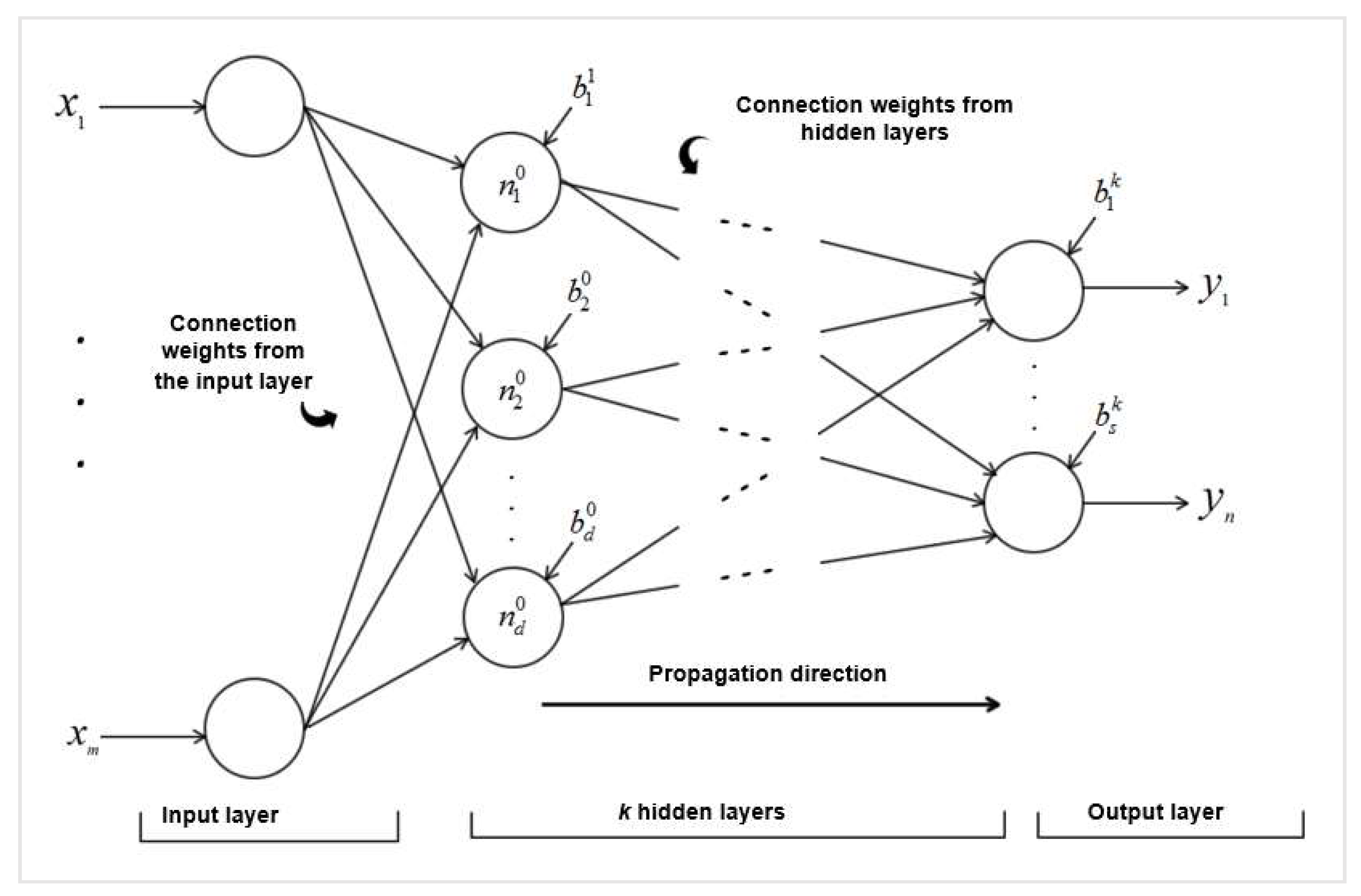
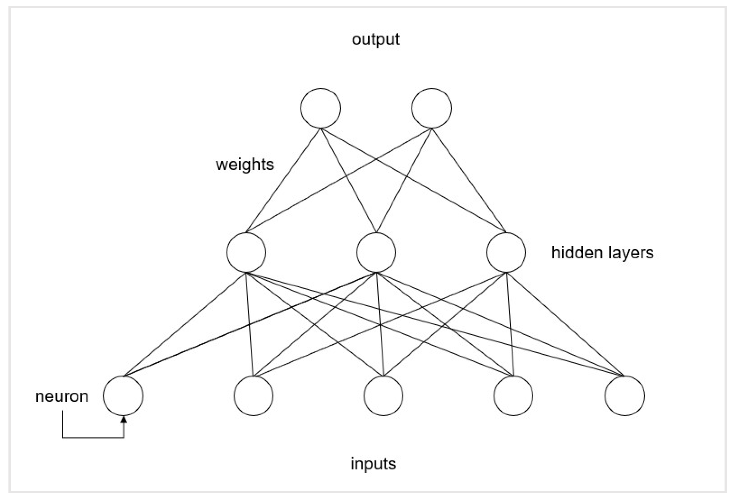
2.2. Artificial Neural Networks (ANN)

ANN algorithms are highly inspired by the sophisticated functioning of human brains, in which information is processed in parallel by billions of interconnected neurons. Neural networks have been applied to several contexts, such as problems with image identification [31], predictability of financial services [32], and even for pattern recognition in DNA [33]. This versatility enables neural networks to solve classification, clustering, or prediction (regression) problems [34].

An ANN is composed of a layer of input neurons, one or more layers of intermediate neurons (hidden layers), and a layer of output neurons [34]. Figure 1 illustrates the integration between layers in an ANN model.

Neurons are interconnected and connections are represented by lines that integrate different layers of the model. Each connection is associated with a number, called a “weight” of the model. The model output ($h_i$) from each neuron (i) in the hidden layer can be represented by Equation (1):

$$h_i=\sigma ( {\sum }_{j=1}^N{V}_{ij}{x}_j+T_i^{hid })$$

(1)

where:

• σ is the activation function which, besides adding nonlinearity components to the neural network, follows the value assumed by the neuron so that the neural network is not paralyzed by divergent neurons;
• N is the number of input neurons;
• V_ij corresponds to the model weights;
• x_j are the inputs of the input neurons;
• $T_i^{hid}$ is the definition of cut lines for hidden neurons.

One of the most essential elements for implementing a neural network is its training. For this, a sample of input data is separated by the model, which already knows the expected output data. The objective of the training stage is to adjust the weights of the connections between neurons so that an error function is minimized. This error function is usually the sum of the squares of the differences between the outputs obtained and the outputs already known at the beginning of the training [35]. It is common, at the beginning of a project involving ANN, to evaluate different architectures and to select the one that best applies to the problem considered [35].

2.3. Extreme Learning Machines (ELM)

ELM, frequently called single hidden layer feedforward neural network (SLFN), is a learning algorithm for neural networks with a single hidden layer of nodes, feedforward, random choice of hidden node parameters, and computational calculation of the output weights. This algorithm has been widely studied recently due to its capacity for fast learning, good generalization, and high capacity for approximation/classification [36].

The parameters for the hidden layer of nodes in ELM architectures are defined at random and do not need to be adjusted during the training steps. That is, the hidden node layer of the structure can be defined prior to training or acquisition of samples for training [32].

To illustrate the architecture of an ELM, it is possible to use the same image that details an ANN (Figure 1), but only a hidden layer is defined. Figure 2 shows the architecture of an ELM considering the case of k = 1.

Several papers have already demonstrated, in theory, how ELM tends to present better and faster generalization performances when compared to ANN and SVM [37,38]. The authors in [39] showed that a SLFN with a hidden layer of randomly generated neurons and properly adjusted output weights preserves the universal generalization ability of neural networks, even if the parameters of the hidden layers are not updated. In addition, these neural networks set the weights for the architecture much faster [39].

3. Site, Dataset, and Algorithm Preparation

3.1. Site

The city of São Paulo was chosen as the study site for the case study. With 12 million inhabitants, São Paulo is the most populous city in Brazil and presents one of the top 20 highest Gross Domestic Products (GDP) in the world [40]. Therefore, this is possibly one of the most likely regions in the country for fast development of solar photovoltaic distributed systems.

Brazil presents an average annual horizontal radiation of 1800 kWh/m² across its territory, offering a prosperous scenario for solar photovoltaic electricity generation countrywide [41]. Even though the highest radiation is concentrated in the northeast region of the country—an annual average of 2200 kWh/m²—most of the installed capacity of solar panels is already deployed in the southeast region of the country due to its larger population density and high GDP per capita and consequent greater energy consumption. This region presents an annual average of 1600 kWh/m² [42].

3.2. Dataset

For developing this study, a dataset from the Institute of Astronomy, Geophysics and Atmospheric Sciences of the University of São Paulo (IAG-USP) was used. This dataset contains a historical series of meteorological parameters measured in the city of São Paulo, at the geographical coordinates 23°39′ S/46°37′ W.

This dataset was chosen due to its easy access within the University of São Paulo and its capacity for scientific contribution through data analysis in a Brazilian context of machine learning model application. This is also the largest meteorological dataset in Brazil, monitoring meteorological parameters since 1933.

The data were received in the format of 20 text files (comma-separated values), which were split into 1 file for data description and 19 files containing the records for each meteorological parameter individually. Each file for the meteorological parameters presents two columns of data records—the date and time of the measurement acquisition and the measure itself.

The dataset contains measurements for a few parameters, such as hourly precipitation since its implementation in 1933. Since the parameters present different acquisition frequencies and time spans, a shorter version of the dataset was prepared for modeling.

This final version contains 19,359 daily observations registered from 1962 to 2014 containing ten meteorological parameters (

Table 1. Dataset description.

Parameter	Dataset Name	Unit
Solar irradiation	irradiation	MJ/m2
Maximum daily temperature	temp_max	°C
Minimum daily temperature	temp_min	°C
Daily maximum wind speeds	wind_daily	m/s
Relative humidity	humidity	%
Daily precipitation	prec	mm
Atmospheric pressure	pressure	atm
Cloud quantity—low altitude	clouds_qtb	-
Cloud quantity—medium altitude	clouds_qtm	-
Cloud quantity—high altitude	clouds_qta	-

):

As a complementary measurement, a last column was added to the dataset that includes the classification of season of the year for each day in the data range, as the target variable for the modeling results, irradiation, is widely dependent on it.

Each meteorological parameter dataset was then cleaned for data points in which there was clearly a measurement problem (e.g., impossible temperature values) or a data maintenance issue (e.g., unusual text in a numeric variable). Both data quality issues were addressed by replacing the daily value of that meteorological parameter with the seven-day moving average value for the seven previous days to the data point.

The dataset summary of each of the variables is presented in

Table 2. Dataset summary.

Measurement	Unit	Minimum Record	1st Quantile	Median	Mean	3rd Quantile	Maximum Record
irradiation	MJ/m2	0	11.93	15.99	16.19	20.49	35.56
temp_max	°C	8.60	22.00	25.50	25.08	28.40	37.20
temp_min	°C	−1.10	12.60	15.20	14.95	17.80	23.20
wind_daily	m/s	0	5	6	6.41	8	28
humidity	%	33.87	76.41	82.15	81.06	87.12	99.25
prec	mm	0	0	0.1	4.1	2.4	146
pressure	Atm	893.6	923.4	925.7	925.8	928.2	939.6
clouds_qtb	-	0	2.22	4.61	4.82	7.39	10.00
clouds_qtm	-	0	0	0.44	1.32	1.94	9.89
clouds_qta	-	0	0	0.11	0.076	1.00	9.94

.

3.3. Algorithm Implementation

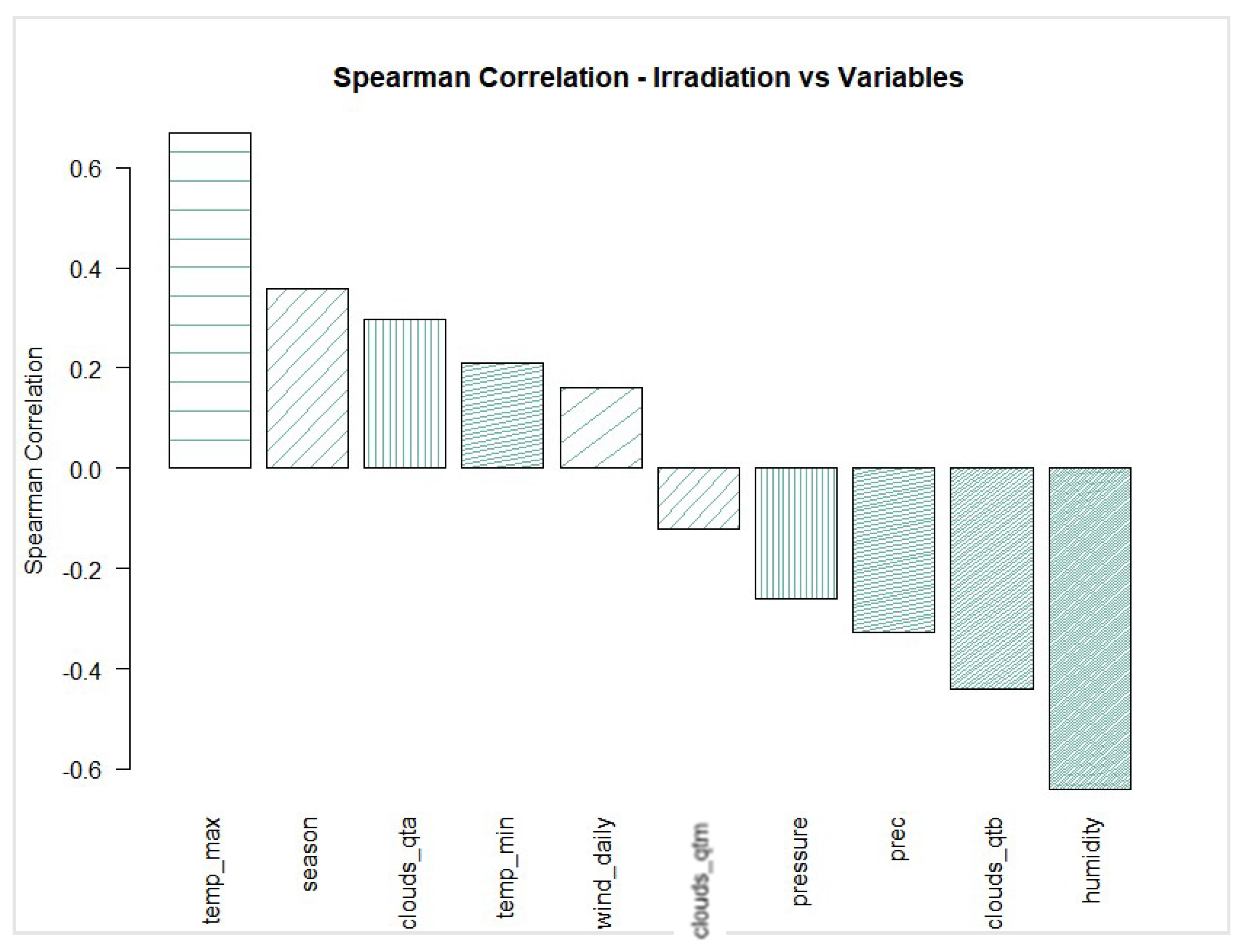
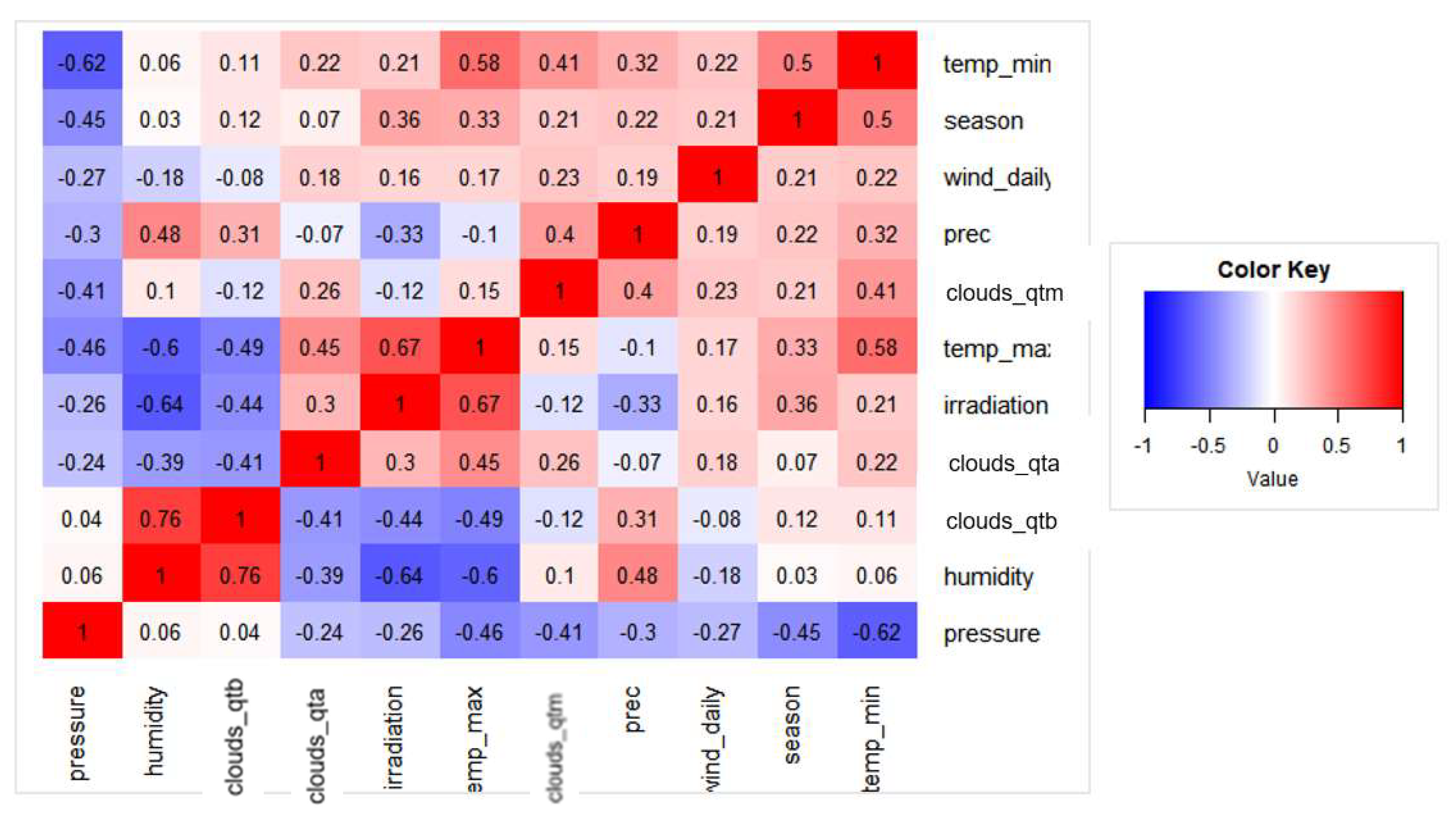
3.3.1. Correlation Analysis

Data ingestion was processed in RStudio, utilizing R language and its libraries for an initial descriptive statistical analysis and further steps, such as model implementation and results evaluation.

Spearman correlation analysis was conducted to understand linear and nonlinear relationships between the meteorological parameters of the dataset and the target variable: irradiation. Figure 3 presents a Spearman correlation matrix heat map considering the variables of the study.

As highlighted, the strongest positive correlation comes from the maximum daily temperature (0.67) and the season of the year (0.36). The strongest negative correlation comes from humidity (−0.64) and number of b-classified clouds (−0.44). Both results are expected since irradiation at a ground level is intrinsically related to ground temperature and the season of the year (higher close to summer). Humidity level and clouds are also expected to act as physical barriers to solar irradiation, reducing the measurements at ground level, where the solar panels would be installed. The correlation between irradiation and each meteorological parameter are used as a premise of feature selection to train the models in the next section.

3.3.2. Algorithm Implementation and Training

All three algorithms, SVM, ANN, and ELM, were implemented in RStudio employing “e1071”, “neuralnet”, and “ELMR” libraries, respectively. A Microsoft Windows 10 operating laptop was used, equipped with an Intel Core i7-8565U CPU @ 1.80 GHz, 16gb of DDR-4 RAM, 256 SSD, and GeForce GTX1650 4Gb GDDR5 Graphics card.

Data preparation was conducted prior to the implementation of each algorithm. First, data were randomly reordered. Then, data columns were normalized aiming to change the meteorological parameter measurements to a common scale, without distorting differences in the ranges of values. Finally, the newly shuffled and normalized dataset was split into training and test datasets based on the quantity of observations: 15,000 to train the models (77.5%) and the 4358 left were allocated to test the algorithm forecasting accuracy (22.5%).

Each forecasting model was composed of the combination of meteorological parameters and the algorithm utilized to predict the irradiation values (SVM, ANN, ELM). Thus, to assess and to compare the performance of each model, three metrics were used: Mean Absolute Error (MAE), Root-Mean-Square Error (RMSE) and Pearson correlation between the actual in situ measured irradiation and the irradiation forecasted by the model. The time spent to train each model was also evaluated, as a metric of model implementation in a real-world application of solar radiation forecasting to support decision-making.

MAE and RMSE are frequently used as metrics to evaluate prediction accuracy for continuous variables [5]. MAE is the average of all the errors in a set of predictions. This average is calculated based on the difference between each predicted value and the actual value observed in the test dataset, considering only the module of the number. MAE is defined by Equation (2):

$$\mathrm{MAE}=\frac{1}{n}{\sum }_{j=1}^n\left| y_i-{\widehat{y}}_j \right|$$

(2)

where:

• n is the number of predicted and observed values;
• y_i = observed value;
• ${\widehat{y}}_j$= predicted value.

RMSE also measures the average magnitude of the error in a sample. However, as the errors are squared before they are averaged, RMSE increases the weight of large errors in the comparison. RMSE is defined by Equation (3):

$$\mathrm{RMSE}=\sqrt{\frac{1}{n}{{\displaystyle \sum }}_{j=1}^n{\left| y_i-{\widehat{y}}_j \right|}^2}$$

(3)

where:

• n is the number of predicted and observed values;
• y_i = observed value;
• ${\widehat{y}}_j$= predicted value.

As a machine learning regression problem, ANN and ELM algorithms were first fine-tuned by optimizing the model parameters. For the ANN, the number of hidden layers and the neuron composition was tweaked. For the ELM, as a single layered neural net, the number of neurons and the activation function were selected to best fit this forecasting problem. Next, the models were confronted to evaluate the impact of the combination and number of meteorological parameters selected to train the model. Comparison metrics were then calculated, evaluating the performance of each model.

4. Results and Discussion

4.1. Modeling Approach

As the criterion for defining a reasonable combination and number of training parameters, a Spearman correlation rank between irradiation and other meteorological variables was created, as represented in Figure 4.

Four different variable groups were defined based on the top positive and negative Spearman correlated parameters, as presented in

Table 3. Meteorological parameter grouping.

Parameter Group Number	Criteria (Figure 4)	Parameters Selected for Model Training
1	Top 1—highest and lowest Spearman correlation	Temp_max + Humidity
2	Top 1 and 2—highest and lowest Spearman correlation	Temp_max + Humidity + Season + Clouds_qtb
3	Top 1, 2, and 3—highest and lowest Spearman correlation	Temp_max + Humidity + Season + Clouds_qtb + clouds_qta + prec
4	All parameters	Temp_max + Humidity + Season + Clouds_qtb + clouds_qta + prec + tem_min + pressure + wind_daily + clouds_qtm

. The general approach was to group sequences of the variables with the highest positive and negative Spearman correlation between irradiation and meteorological parameters, comparing the performance of the irradiation prediction among the groups and number of variables.

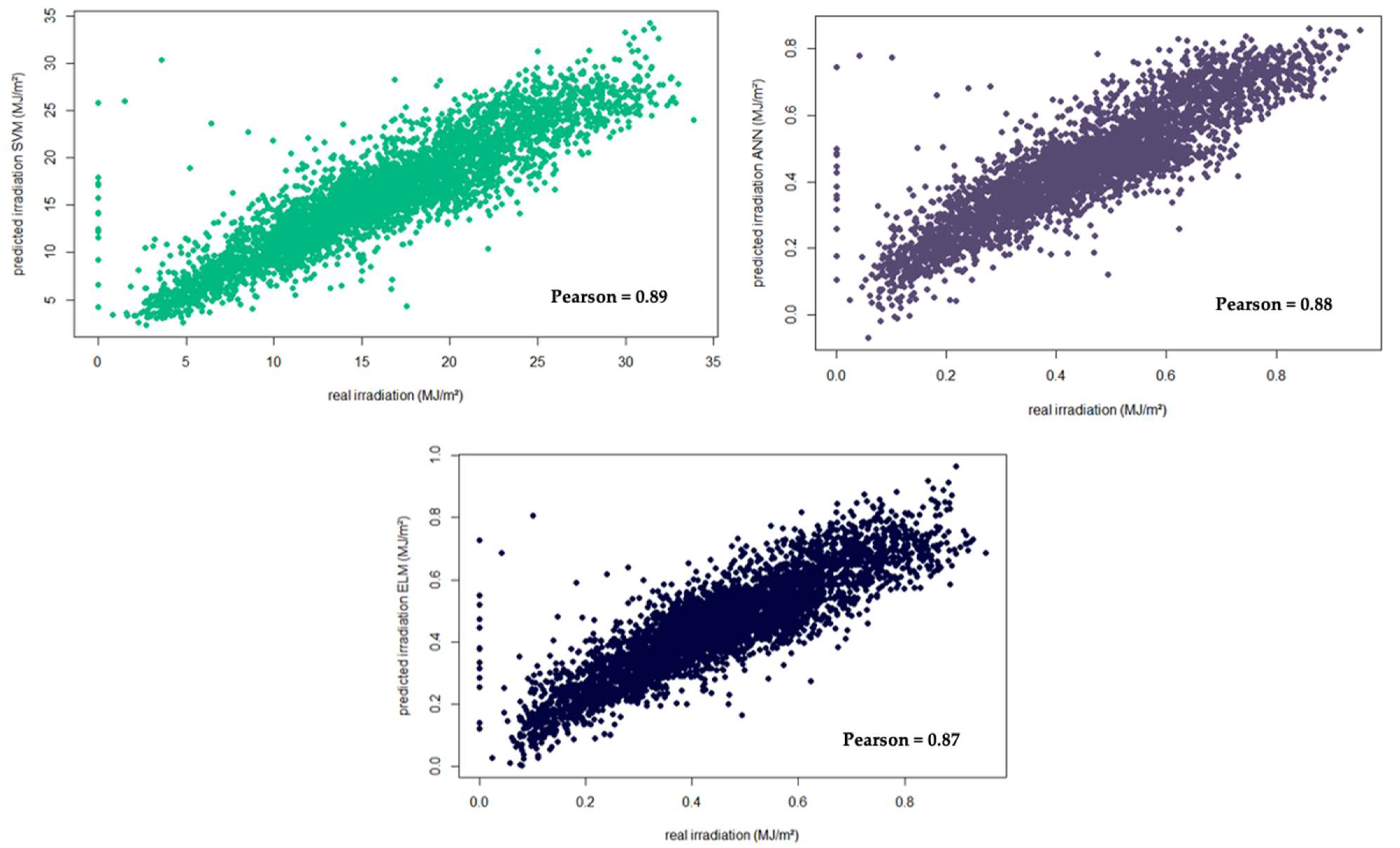
4.2. Modeling Results

After defining the groups of parameters and fine-tuning the models, SVM was the first algorithm trained and tested.

Table 4. SVM forecasting results.

Support Vector Machines (SVM)
Model	Parameter Group	MAE [MJ/m2]	RMSE [MJ/m2]	Pearson Correlation	Training Time [s]
SVM_1	1	3.08	4.15	0.76	29.15
SVM_2	2	2.54	3.43	0.84	28.99
SVM_3	3	2.41	3.24	0.86	28.66
SVM_4	4	2.05	2.78	0.89	35.10

summarizes and compares the results for all the SVM models.

First, an increasing accuracy of the forecasting directly proportional to the number of meteorological parameters used to train the model is clearly noticed. SVM_4 is the model that best predicts the target irradiation variable, presenting a MAE of 2.05 W/m² or 12.7% of the average irradiation value in the time series—16.19 W/m². As the number of parameters increases, there is almost no relative incremental training time for the models.

Multiple setups of ANN were tested and the best parameters for the proposed forecasting problem were hyperbolical tangent as the activation function, 5 neurons in the first hidden layer, 2 hidden layers, and 0.5 as the threshold. Increasing the number of neurons, hidden layers, and reducing the threshold causes practically no impact on the forecasting results at a very high computational cost. A reduction in the threshold from 0.5 to 0.1, for example, reduced the MAE from 3.13 to 3.09, taking 55 times the training time.

Table 5. ANN forecasting results for 5 neurons in the first hidden layer, 2 hidden layers, and 0.5 threshold.

Artificial Neural Network (ANN)
Model	Parameter Group	MAE [MJ/m2]	RMSE [MJ/m2]	Pearson Correlation	Training Time [s]
ANN_1	1	3.13	4.12	0.76	16.6
ANN_2	2	2.70	0.36	0.83	25.9
ANN_3	3	2.67	3.48	0.83	39.6
ANN_4	4	2.24	2.99	0.88	29.4

summarizes and compares the results for the selected ANN model and the groups of meteorological parameters.

ANN presented a similar training rate when compared to SVM, at an average of 28 s to complete. The behavior related to the number of meteorological parameters is also very similar to SVM, presenting reduced errors as they increase in the model. The Pearson correlation and MAE/RMSE are slightly lower when compared to each parameter group. The MAE for ANN_4, the best ANN predicting model, is 13.8% of the average irradiation value in the time series.

As developed for the ANN setup, the best regression ELM to the problem was configured considering the sine function as the activation function: size 50 of the first block to be processed, size 50 of each chunk to be processed at each step, and 100 neurons at the hidden layer.

Table 6. ELM forecasting results considering the sine function as the activation function: size 50 of the first block to be processed, size 50 of each chunk to be processed at each step, and 100 neurons at the hidden layer.

Extreme Learning Machine (ELM)
Model	Parameter Group	MAE [MJ/m2]	RMSE [MJ/m2]	Pearson Correlation	Training Time [s]
ELM_1	1	3.31	4.30	0.73	3.27
ELM_2	2	2.84	3.73	0.80	1.35
ELM_3	3	2.77	3.63	0.82	1.19
ELM_4	4	2.35	3.09	0.87	1.15

summarizes and compares the results for all the ELM models.

The learning rate of the ELM algorithm is impressive; it can reduce the average training time by 94.3% compared to SVM and 93.8% compared to ANN training rates. Note that as the number of variables used to train the model increases, the learning time is reduced, as the accuracy of the model grows. Thus, ELM presents consistent accuracy when trained with all the available meteorological parameters at almost no processing cost. The MAE for ELM_4 is 14.5% of the average irradiation value in the time series.

All the algorithms introduced their best forecasting performance when all the meteorological parameters were added to the models, showing that they all contribute to the prediction accuracy. As shown in Figure 5, the prediction results for SVM, ANN, and ELM are close when trained with the same group of meteorological parameters.

5. Conclusions and Future Work

All the algorithms used presented good results when trained with all the meteorological parameters; however, when exploring their performance in an actual case study for the city of São Paulo, Brazil, SVM produced the lowest RMSE and ELM the fastest training rate.

Even though the performance of SVM, ANN, and ELM were similar, SVM presents the best results with no considerable increase in training time. For solar electricity generating capacity planning purposes, the algorithms most frequently used in the literature presented a similar performance when trained with data for the city of São Paulo.

The literature also suggests that ELM is expected to play a significant role on solar forecasting due to its fast-training ability and ease of implementation. The results presented herein for the city of São Paulo show ELM can reduce the average training time by 94.3% compared to SVM, and 93.8% compared to ANN training rates. However, the RMSE rises to 3.3% and 11.1% when compared to ANN and SVM, respectively.

As the number of training parameters increases, so do the accuracy of the models. The best predicting models for all three algorithms are trained with all the data available for the site, there being 10 available meteorological parameters responsible for the improvement in results.

It can also be concluded that the extensive dataset from the University of São Paulo played a good role in providing data for training a ML forecasting model. Therefore, for local and regional deployment of solar photovoltaic generating facilities, this public dataset can play a significant role in reducing the uncertainties of solar resource natural variability.

Future Research Directions

As the number of meteorological parameters plays a significant role in the forecasting accuracy, there is an opportunity to further evaluate the impact of adding other parameters to the models as they become available by the meteorological measuring station.

In Brazil, the energy planning exercise is conducted at a national level, considering local specificities, such as resource availability, electricity demand, and social/environmental impact. Therefore, there is similarly an opportunity to assess the performance of the same models in other sites for the country to integrate the forecasting exercise and to maximize the performance of the models.

Finally, quality of data is also a major concern when these models are trained and operated for decision-making. There is an opportunity for considering the impact of data quality on the performance of the models. Further steps of this work contemplate understanding data quality dimensions, such as completeness, uniqueness, validity, accuracy, consistency, and timeliness, besides their relationship with forecasting solar radiation for solar photovoltaic electricity generation.

References

1. IRENA; ADFD. Advancing Renewables in Developing Countries: Progress of Projects Supported through the IRENA/ADFD Project Facility; International Renewable Energy Agency (IRENA); Abu Dhabi Fund for Development (ADFD): Abu Dhabi, United Arab Emirates, 2020.
2. IRENA. Renewable Capacity Statistics 2019; International Renewable Energy Agency (IRENA): Abu Dhabi, United Arab Emirates, 2019. [Google Scholar]
3. EPE. O Compromisso Do Brasil No Combate às Mudanças Climáticas: Produção e Uso de Energia; Empresa de Pesquisa Energética: Rio de Janeiro, Brazil, 2016. [Google Scholar]
4. MME/EPE. Plano Decenal de Expansão de Energia 2027/Ministério de Minas e Energia; Empresa de Pesquisa Energética: Rio de Janeiro, Brazil, 2018. [Google Scholar]
5. Shuo, L.; Jun, M.; Xiong, M.; Hui, H.G.; Wei, H.R. The platform of monitoring and analysis for solar power data. In Proceedings of the 2016 China International Conference on Electricity Distribution (CICED), Xi’an, China, 10–13 August 2016. [Google Scholar] [CrossRef]
6. Haupt, S.; Kosovic, B. Variable Generation Power Forecasting as a Big Data Problem. IEEE Trans. Sustain. Energy 2017, 8, 725–732. [Google Scholar] [CrossRef]
7. Singh, B.; Dwivedi, S.; Hussain, I.; Verma, A.K. Grid integration of solar PV power generating system using QPLL based control algorithm. In Proceedings of the 2014 6th IEEE Power India International Conference (PIICON), Delhi, India, 5–7 December 2014; pp. 1–6. [Google Scholar] [CrossRef]
8. Francisco, A.C.C.; de Miranda Vieira, H.E.; Romano, R.R.; Roveda, S.R.M.M. Influência de Parâmetros Meteorológicos na Geração de Energia em Painéis Fotovoltaicos: Um Caso de Estudo do Smart Campus Facens, SP. 2019. Available online: https://www.scielo.br/j/urbe/a/f5NZ33Mv5FNCFVpjjv6DsSn/?lang=pt (accessed on 5 July 2021).
9. Revankar, P.S.; Thosar, A.G.; Gandhare, W.Z. Maximum Power Point Tracking for PV Systems Using MATALAB/SIMULINK. In Proceedings of the 2010 Second International Conference on Machine Learning and Computing, Bangalore, India, 9–11 February 2010; pp. 8–11. [Google Scholar] [CrossRef]
10. Chia, Y.; Lee, L.; Shafiabady, N.; Isa, D. A load predictive energy management system for supercapacitor-battery hybrid energy storage system in solar application using the Support Vector Machine. Appl. Energy 2015, 137, 588–602. [Google Scholar] [CrossRef]
11. Simmhan, Y.; Aman, S.; Kumbhare, A.; Liu, R.; Stevens, S.; Zhou, Q.; Prasanna, V. Cloud-Based Software Platform for Big Data Analytics in Smart Grids. Comput. Sci. Eng. 2013, 15, 38–47. [Google Scholar] [CrossRef]
12. Aybar-Ruiz, A.; Jiménez-Fernández, S.; Cornejo-Bueno, L.; Casanova-Mateo, C.; Sanz-Justo, J.; Salvador-González, P.; Salcedo-Sanz, S. A novel Grouping Genetic Algorithm–Extreme Learning Machine approach for global solar radiation prediction from numerical weather models inputs. Sol. Energy 2016, 132, 129–142. [Google Scholar] [CrossRef]
13. Burianek, T.; Stanislav, M. Solar Irradiance Forecasting Model Based on Extreme Learning Machine. In Proceedings of the 2016 IEEE 16th International Conference on Environment and Electrical Engineering (EEEIC), Florence, Italy, 7–10 June 2016. [Google Scholar] [CrossRef]
14. Shamshirband, S.; Mohammadi, K.; Yee, P.; Petković, D.; Mostafaeipour, A. A comparative evaluation for identifying the suitability of extreme learning machine to predict horizontal global solar radiation. Renew. Sustain. Energy Rev. 2015, 52, 1031–1042. [Google Scholar] [CrossRef]
15. Kitchenham, B.; Charters, S. Guidelines for Performing Systematic Literature Reviews in Software Engineering. 2007. Available online: https://userpages.uni-koblenz.de/~laemmel/esecourse/slides/slr.pdf (accessed on 7 June 2020).
16. de Freitas Viscondi, G.; Alves-Souza, S.N. A Systematic Literature Review on big data for solar photovoltaic electricity generation forecasting. Sustain. Energy Technol. Assess. 2019, 31, 54–63. [Google Scholar] [CrossRef]
17. Belaid, S.; Mellit, A. Prediction of daily and mean monthly global solar radiation using support vector machine in an arid climate. Energy Convers. Manag. 2016, 118, 105–118. [Google Scholar] [CrossRef]
18. Chow, S.K.H.; Lee, E.W.M.; Li, D.H.W. Short-Term Prediction of Photovoltaic Energy Generation by Intelligent Approach. Energy Build. 2012, 55, 660–667. [Google Scholar] [CrossRef]
19. Yadav, A.K.; Chandel, S.S. Solar radiation prediction using Artificial Neural Network techniques: A review. Renew. Sustain. Energy Rev. 2014, 33, 772–781. [Google Scholar] [CrossRef]
20. Khatib, T.; Mohamed, A.; Sopian, K.; Mahmoud, M. Assessment of Artificial Neural Networks for Hourly Solar Radiation Prediction. Int. J. Photoenergy 2012, 2012, 946890. [Google Scholar] [CrossRef]
21. Melzi, F.N.; Touati, T.; Same, A.; Oukhellou, L. Hourly Solar Irradiance Forecasting Based on Machine Learning Models. In Proceedings of the 2016 15th IEEE International Conference on Machine Learning and Applications (ICMLA), Anaheim, CA, USA, 18–20 December 2016. [Google Scholar] [CrossRef]
22. Al-Dahidi, S.; Ayadi, O.; Adeeb, J.; Alrbai, M.; Qawasmeh, B.R. Extreme Learning Machines for Solar Photovoltaic Power Predictions. Energies 2018, 10, 2725. [Google Scholar] [CrossRef] [Green Version]
23. Huang, G.-B.; Zhu, Q.; Siew, C. Extreme Learning Machine: Theory and Applications. Neurocomputing 2006, 70, 489–501. [Google Scholar] [CrossRef]
24. Pasion, C.; Wagner, T.; Koschnick, C.; Schuldt, S.; Williams, J.; Hallinan, K. Machine Learning Modeling of Horizontal Photovoltaics Using Weather and Location Data. Energies 2020, 13, 2570. [Google Scholar] [CrossRef]
25. Mahesh, B. Machine Learning Algorithms—A Review. Int. J. Sci. Res. 2019, 9, 381–386. [Google Scholar]
26. IDC. Worldwide Global DataSphere Forecast, 2021–2025: The World Keeps Creating More Data—Now, What Do We Do with It All? International Data Corporation (IDC): Needham, MA, USA, 2021. [Google Scholar]
27. Boser, B.E.; Guyon, I.M.; Vapnik, V.N. A training algorithm for optimal margin classifiers. In Proceedings of the Fifth Annual Workshop on Computational Learning Theory-COLT’92, Pittsburgh, PA, USA, 27 July 1992. [Google Scholar] [CrossRef]
28. Lorena, A.C.; de Carvalho, A.C.P.L.F. Uma introdução às Support Vector Machines. In Revista de Informática Aplicada e Teórica; Universidade Federal do Rio Grande do Sul: Porto Alegre, Brazil, 2007. [Google Scholar]
29. Steinwart, I.; Christmann, A. Support Vector Machines. Information Science and Statistics; Springer Science & Business Media: Berlin, Germany, 2008. [Google Scholar] [CrossRef]
30. Noble, W.S. What is a support vector machine? Nat. Biotechnol. 2006, 24, 1565–1567. [Google Scholar] [CrossRef] [PubMed]
31. Namba, M.; Zhang, Z. Cellular Neural Network for Associative Memory and Its Application to Braille Image Recognition. In Proceedings of the 2006 IEEE International Joint Conference on Neural Network Proceedings, Vancouver, BC, Canada, 16–21 July 2006. [Google Scholar] [CrossRef]
32. Odom, M.D.; Sharda, R. A neural network model for bankruptcy prediction. In Proceedings of the 1990 IJCNN International Joint Conference on Neural Networks, San Diego, CA, USA, 17–21 June 1990. [Google Scholar] [CrossRef]
33. Cherry, K.M.; Qian, L. Scaling up molecular pattern recognition with DNA-based winner-take-all neural networks. Nature 2018, 559, 370–376. [Google Scholar] [CrossRef] [PubMed]
34. Wang, S.-C. Artificial Neural Network. In Interdisciplinary Computing in Java Programming; Springer: Boston, MA, USA, 2003; pp. 81–100. [Google Scholar] [CrossRef]
35. Ripley, B.D. Pattern Recognition and Neural Networks; Cambridge University Press: Cambridge, UK, 1996. [Google Scholar]
36. Tang, J.; Deng, C.; Huang, G.-B. Extreme Learning Machine for Multilayer Perceptron. In IEEE Transactions on Neural Networks and Learning Systems; IEEE: Piscataway, NJ, USA, 2016; Volume 27, pp. 809–821. [Google Scholar] [CrossRef]
37. Huang, G.-B.; Zhou, H.; Ding, X.; Zhang, R. Extreme learning machine for regression and multiclass classification. IEEE Trans. Syst. Man Cybern. Part B Cybern. 2012, 42, 513–529. [Google Scholar] [CrossRef] [PubMed] [Green Version]
38. Huang, G.-B. An Insight into Extreme Learning Machines: Random Neurons, Random Features and Kernels. Cogn. Comput. 2014, 6, 376–390. [Google Scholar] [CrossRef]
39. Huang, G.-B.; Chen, L.; Siew, C.-K. Universal approximation using incremental constructive feedforward networks with random hidden nodes. IEEE Trans. Neural Netw. 2006, 17, 879–892. [Google Scholar] [CrossRef] [PubMed] [Green Version]
40. São Paulo será 6ª Cidade Mais Rica do Mundo até 2025. Price Waterhouse & Coopers e BBC Brasil. November 2009. Available online: https://www.bbc.com/portuguese/noticias/2009/11/091109_ranking_cidades_price_rw (accessed on 4 July 2021).
41. IEA. Next Generation Wind and Solar Power from Cost to Value; International Energy Agency: Paris, France, 2016. [Google Scholar]
42. CPI. Developing Brazil’s Market for Distributed Solar Generation Climate Policy Initiative. 2017. Available online: https://www.oecd.org/publications/next-generation-wind-and-solar-power-9789264258969-en.htm (accessed on 4 July 2021).
Figure 1. General architecture of a neural network.
Energies 14 05657 g001
Figure 2. General architecture of an extreme learning machine.
Energies 14 05657 g002
Figure 3. Heat m ap: Spearman correlation matrix.
Energies 14 05657 g003
Figure 4. Spearman correlation between irradiation and meteorological parameters.
Energies 14 05657 g004
Figure 5. Predicted irradiation versus real measured irradiation when all the meteorological parameters were applied to the models. SVM (upper right), ANN (upper left) and ELM (lower center).
Energies 14 05657 g005